
Angle Estimation for Range-Spread Targets Based on Scatterer Energy Focusing


Abstract
1. Introduction
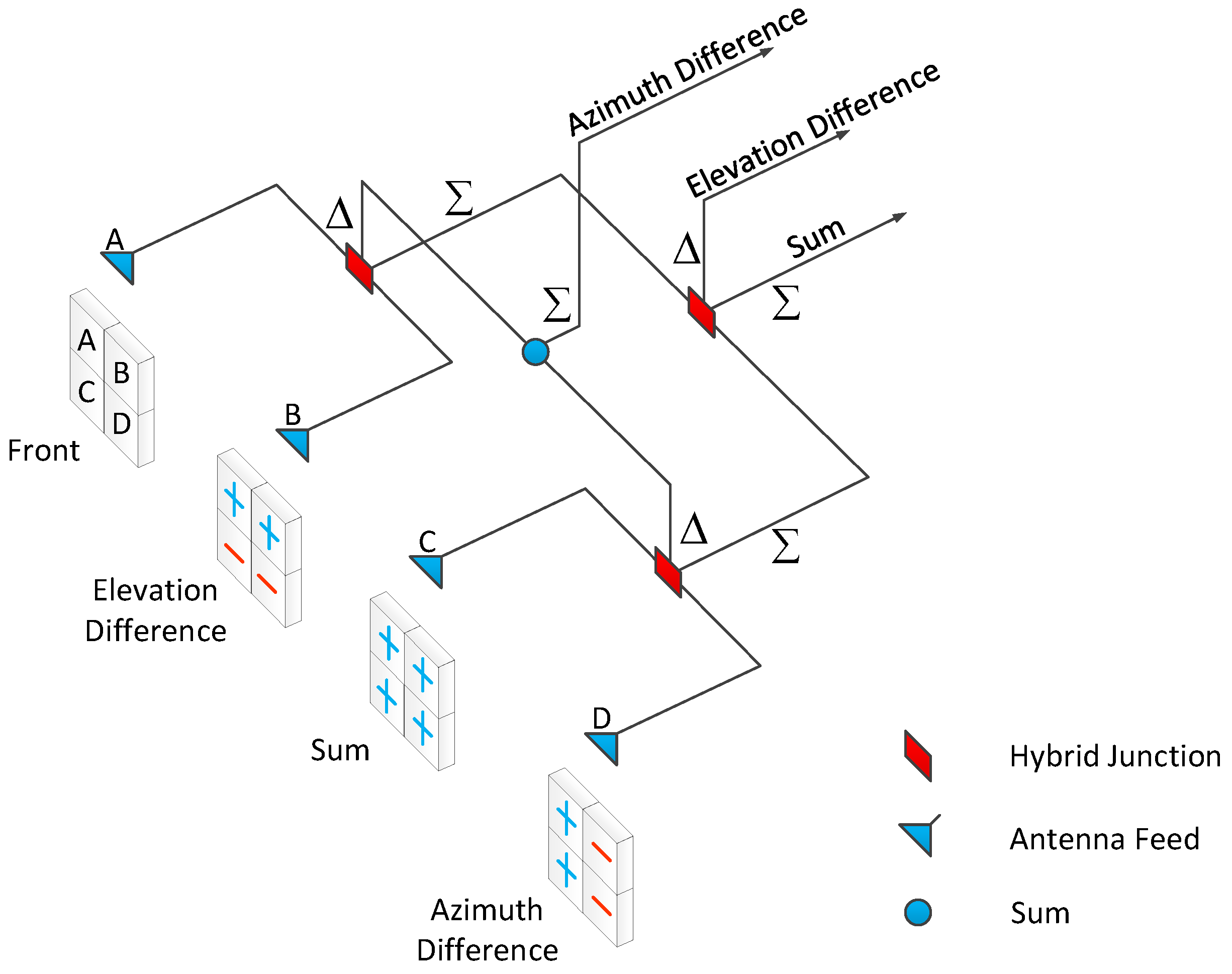
2. Conventional Monopulse Amplitude Comparison Angle Estimation
3. Angle Estimation Based on Scatterer Energy Focusing
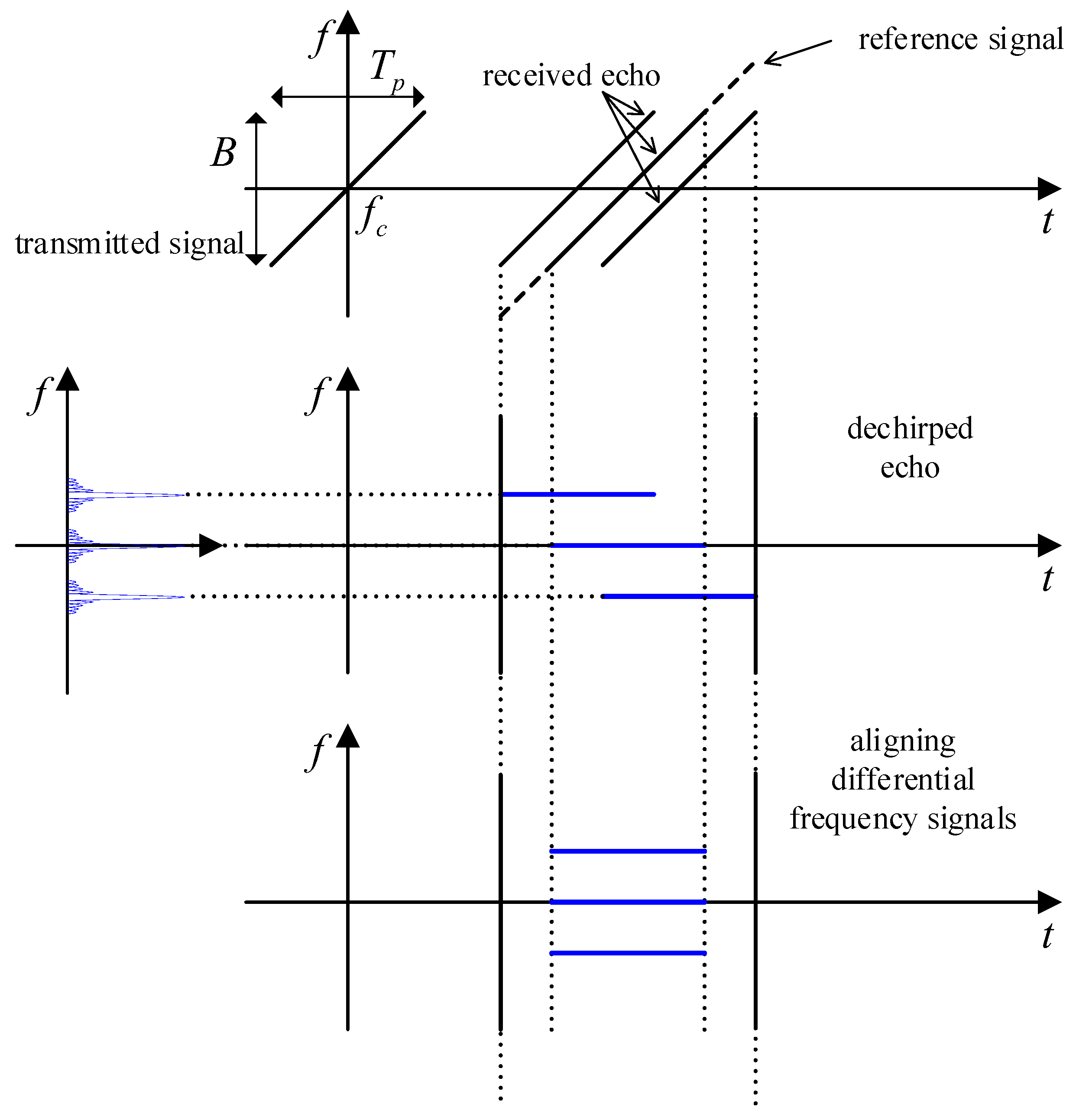
3.1. Range-Spread Target Signal Model
3.2. Theoretical Deduction
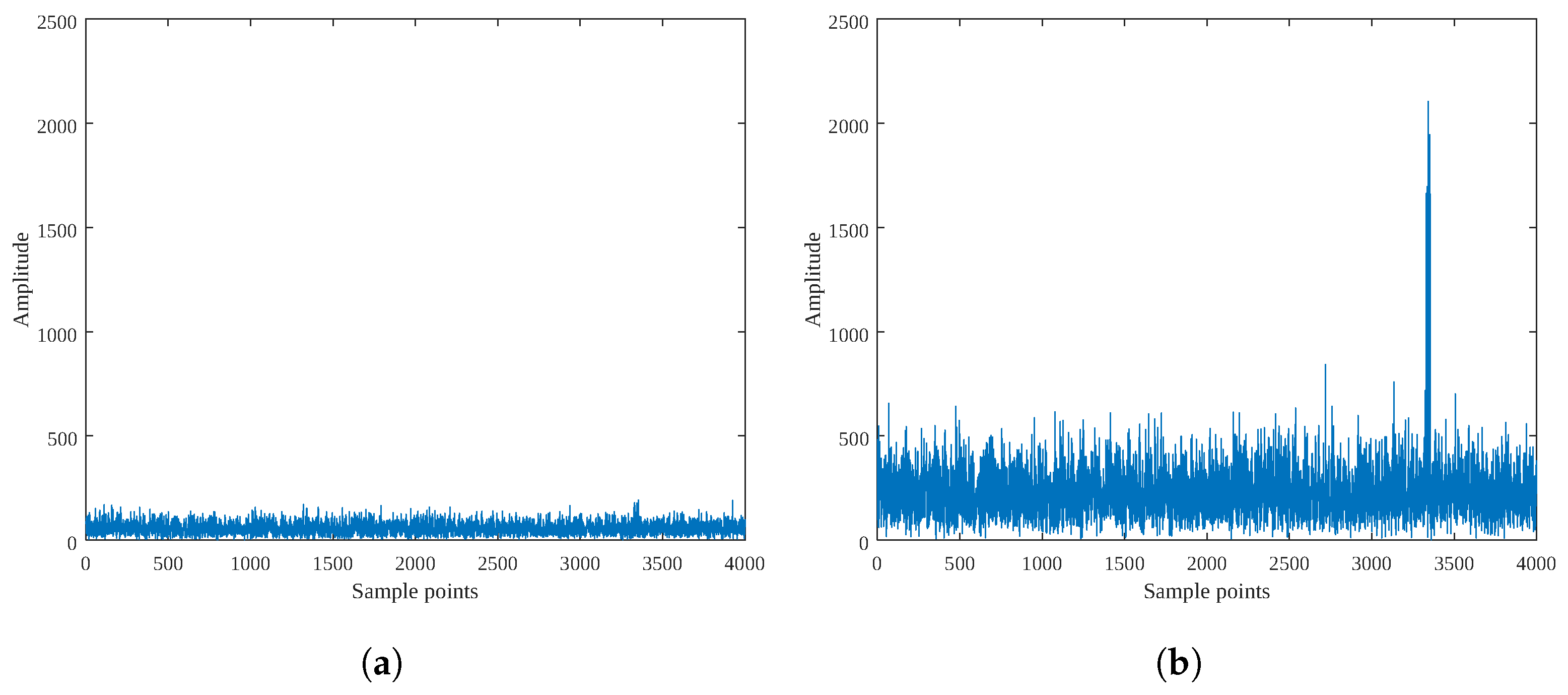
3.2.1. Energy-Focusing Detector
3.2.2. Energy-Focusing Angle Estimation
3.3. Detector Performance Analysis
3.4. Signal-to-Noise Ratio Analysis
3.5. Root Mean Square Error
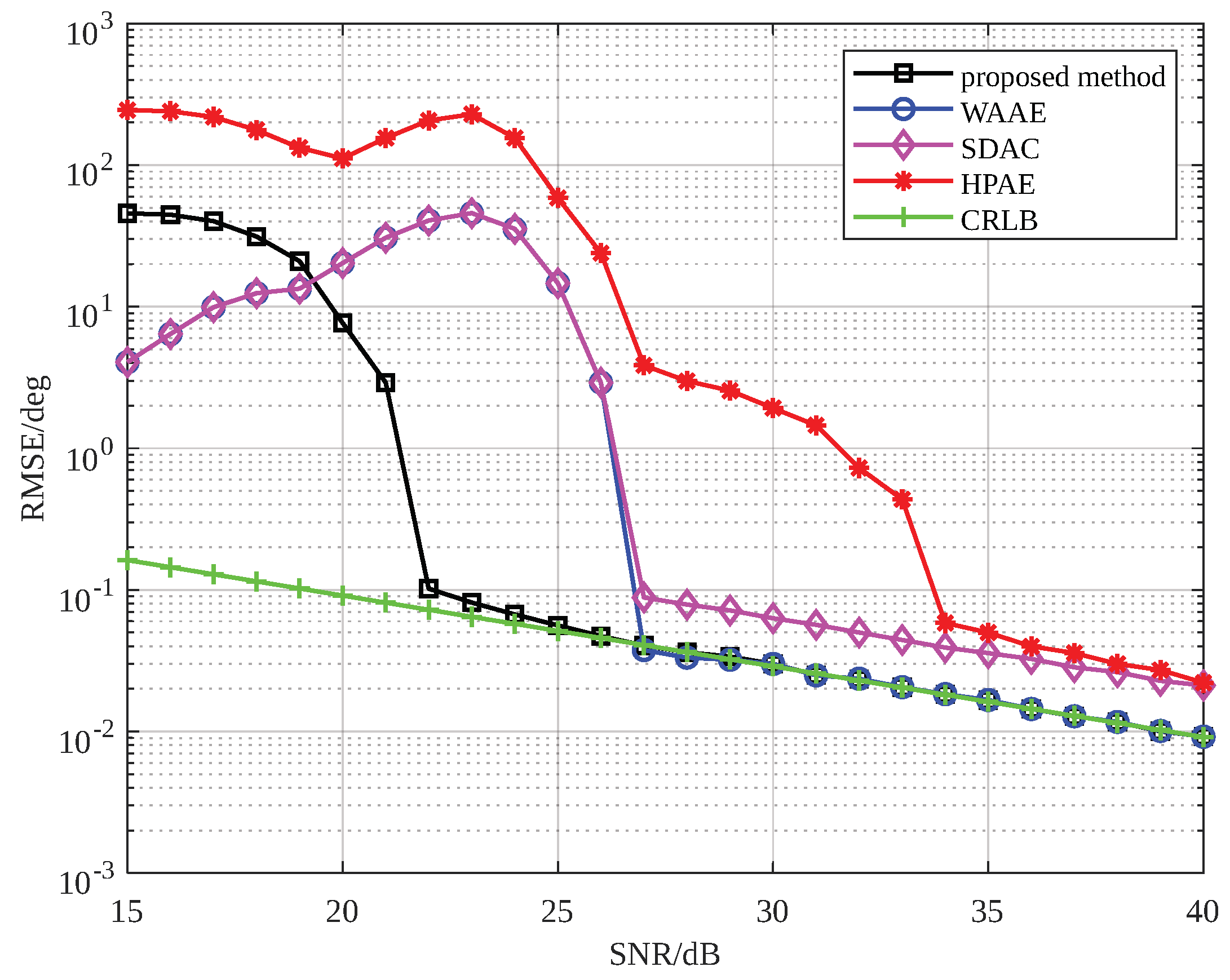
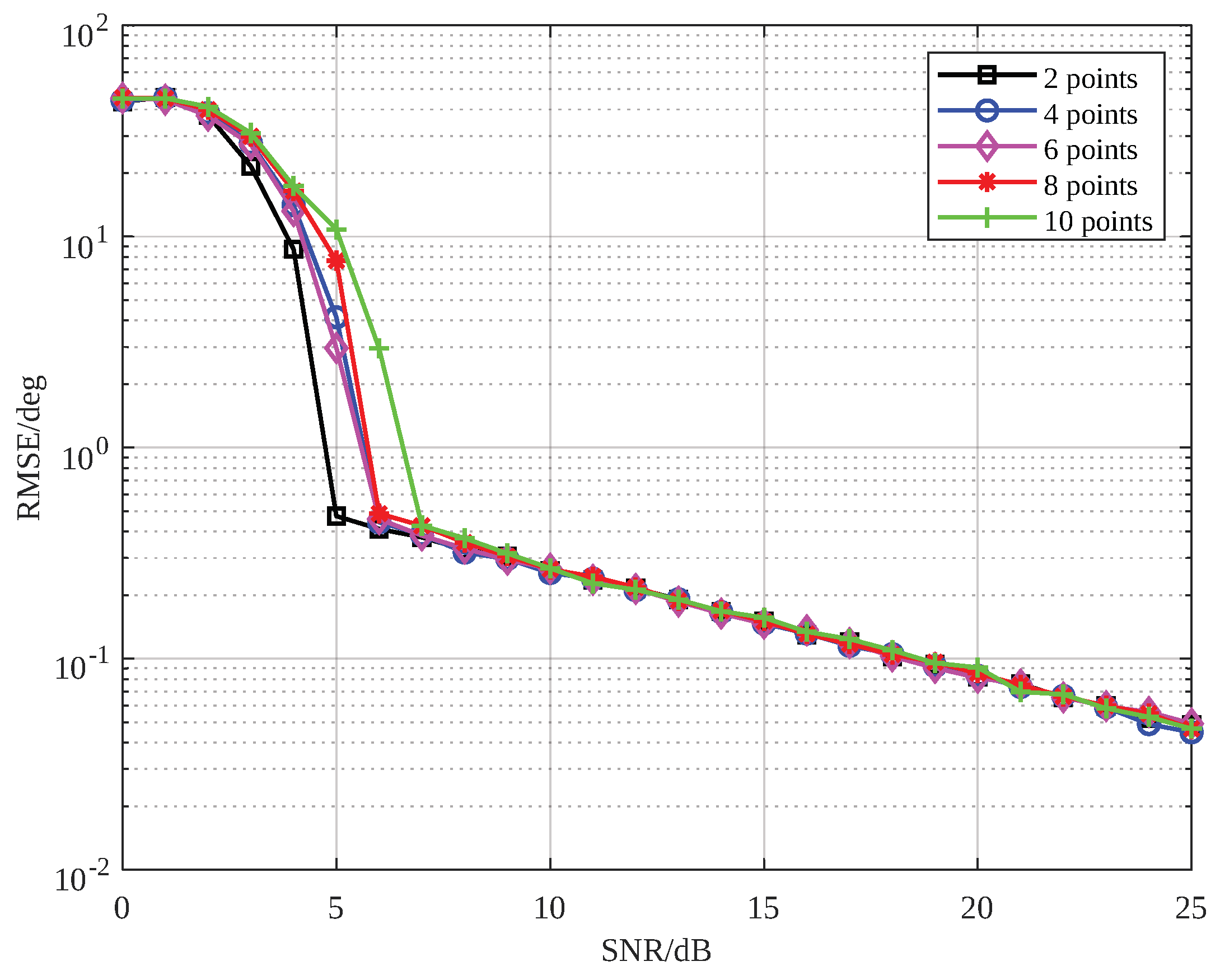
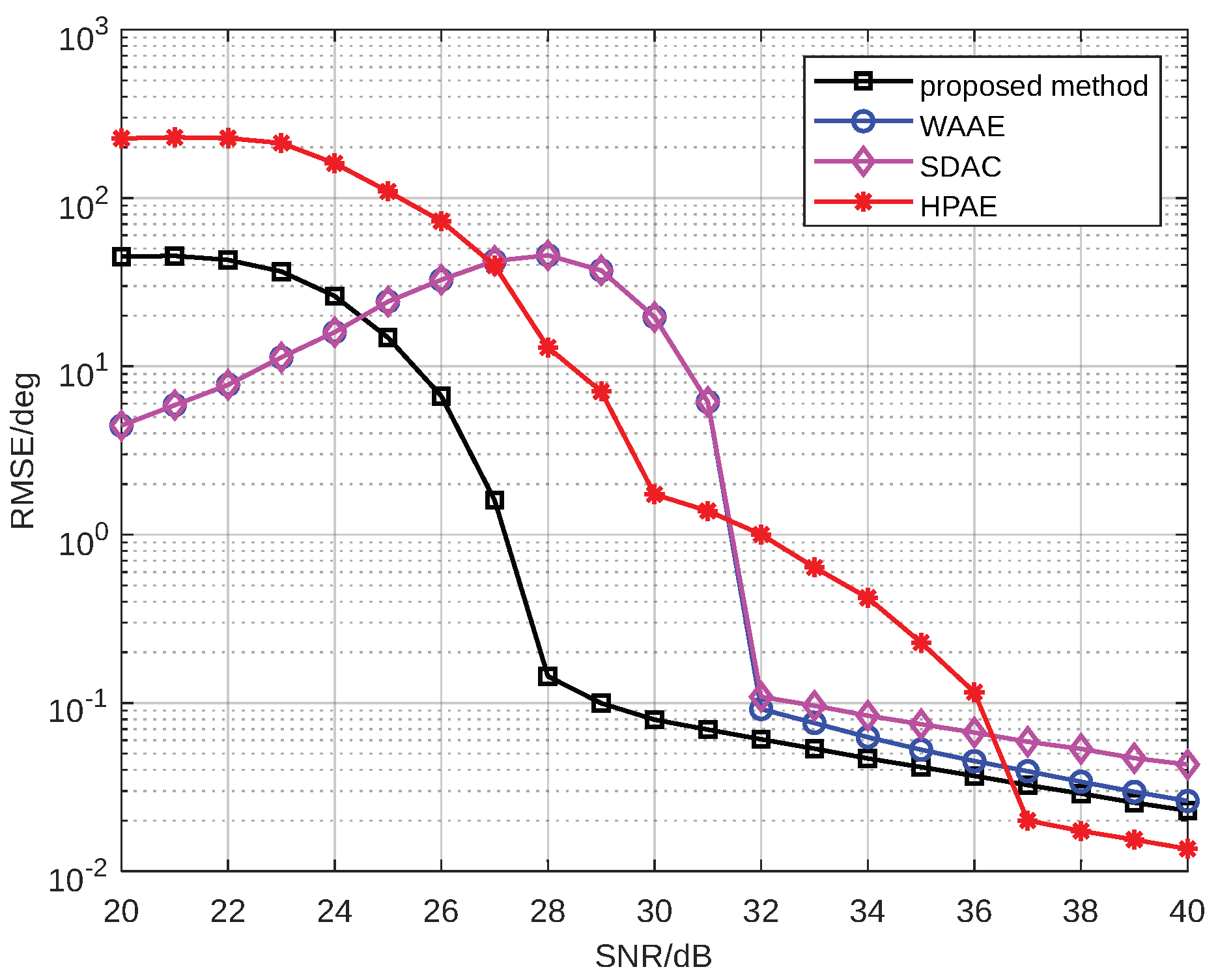
4. Simulation Results
5. Conclusions
Author Contributions
Funding
Institutional Review Board Statement
Informed Consent Statement
Data Availability Statement
Conflicts of Interest
References
- Mahafza, B.R.; Elsherbeni, A. MATLAB Simulations for Radar Systems Design; Chapman and Hall/CRC: Boca Raton, FL, USA, 2003. [Google Scholar]
- Cai, J.; Wang, R.; Yang, H. Angle Expansion Estimation and Correction Based on the Lindeberg–Feller Central Limit Theorem Under Multi-Pulse Integration. Remote Sens. 2024, 16, 4535. [Google Scholar] [CrossRef]
- Yoon, Y.S. Elevation Angle Estimation in a Multipath Environment Using MIMO-OFDM Signals. Remote Sens. 2024, 16, 4490. [Google Scholar] [CrossRef]
- Li, W.; Xu, X.; Xu, Y.; Luan, Y.; Tang, H.; Chen, L.; Zhang, F.; Liu, J.; Yu, J. Angle Estimation Using Learning-Based Doppler Deconvolution in Beamspace with Forward-Looking Radar. Remote Sens. 2024, 16, 2840. [Google Scholar] [CrossRef]
- Zhang, Y.X.; Hong, R.J.; Pan, P.P.; Deng, Z.M.; Liu, Q.F. Frequency-domain range sidelobe correction in stretch processing for wideband LFM radars. IEEE Trans. Aerosp. Electron. Syst. 2017, 53, 111–121. [Google Scholar] [CrossRef]
- Jian, T.; He, Y.; Su, F.; Qu, C.; Ping, D. Cascaded detector for range-spread target in non-Gaussian clutter. IEEE Trans. Aerosp. Electron. Syst. 2012, 48, 1713–1725. [Google Scholar] [CrossRef]
- Tullsson, B.E. Monopulse tracking of Rayleigh targets: A simple approach. IEEE Trans. Aerosp. Electron. Syst. 1991, 27, 520–531. [Google Scholar] [CrossRef]
- Blair, W.; Brandt-Pearce, M. Statistical description of monopulse parameters for tracking Rayleigh targets. IEEE Trans. Aerosp. Electron. Syst. 1998, 34, 597–611. [Google Scholar] [CrossRef]
- Blair, W.D.; Brandt-Pearce, M. Monopulse DOA estimation of two unresolved Rayleigh targets. IEEE Trans. Aerosp. Electron. Syst. 2001, 37, 452–469. [Google Scholar] [CrossRef]
- Ham, H.W.; Lee, J.H. Improvement of performance analysis of amplitude-comparison monopulse algorithm in the presence of an additive noise. Electronics 2021, 10, 2649. [Google Scholar] [CrossRef]
- Kim, M.; Hong, D.; Park, S. A study on the amplitude comparison monopulse algorithm. Appl. Sci. 2020, 10, 3966. [Google Scholar] [CrossRef]
- Lee, S.H.; Lee, S.J.; Choi, I.O.; Kim, K.T. ICA-based phase-comparison monopulse technique for accurate angle estimation of multiple targets. IET Radar Sonar Navig. 2018, 12, 323–331. [Google Scholar] [CrossRef]
- Islam, S.M.; Yavari, E.; Rahman, A.; Lubecke, V.M.; Boric-Lubecke, O. Multiple subject respiratory pattern recognition and estimation of direction of arrival using phase-comparison monopulse radar. In Proceedings of the 2019 IEEE Radio and Wireless Symposium (RWS), Orlando, FL, USA, 20–23 January 2019; pp. 1–4. [Google Scholar]
- Zhang, Y.X.; Liu, Q.F.; Hong, R.J.; Pan, P.P.; Deng, Z.M. A novel monopulse angle estimation method for wideband LFM radars. Sensors 2016, 16, 817. [Google Scholar] [CrossRef] [PubMed]
- Xiong, X.; Deng, Z.; Qi, W.; Dou, Y. High-precision angle estimation based on phase ambiguity resolution for high resolution radars. Sci. China Inf. Sci. 2019, 62, 40307. [Google Scholar] [CrossRef]
- An, Q.; Yeh, C.; Lu, Y.; He, Y.; Yang, J. Time-Varying Angle Estimation of Multiple Unresolved Extended Targets via Monopulse Radar. IEEE Trans. Aerosp. Electron. Syst. 2024, 60, 4650–4667. [Google Scholar] [CrossRef]
- Kohler, M.; Saam, A.; Worms, J.; O’Hagan, D.W.; Bringmann, O. Wideband direction of arrival estimation using monopulse in Rotman lens beamspace. In Proceedings of the 2019 International Radar Conference (RADAR), Toulon, France, 23–27 September 2019; pp. 1–5. [Google Scholar]
- Tianyi, C.; Bo, D.; Weibo, H. Super-resolution parameter estimation of monopulse radar by wide-narrowband joint processing. J. Syst. Eng. Electron. 2023, 34, 1158–1170. [Google Scholar] [CrossRef]
- Liu, Y.; Tan, Z.W.; Khong, A.W.; Liu, H. Joint source localization and association through overcomplete representation under multipath propagation environment. In Proceedings of the ICASSP 2022-2022 IEEE International Conference on Acoustics, Speech and Signal Processing (ICASSP), Singapore, 23–27 May 2022; pp. 5123–5127. [Google Scholar]
- Zamani, H.; Zayyani, H.; Marvasti, F. An iterative dictionary learning-based algorithm for DOA estimation. IEEE Commun. Lett. 2016, 20, 1784–1787. [Google Scholar] [CrossRef]
- Battaglia, G.M.; Isernia, T.; Palmeri, R.; Morabito, A.F. Synthesis of orbital angular momentum antennas for target localization. Radio Sci. 2023, 58, 1–15. [Google Scholar] [CrossRef]
- Zhang, Y.; Xu, W.; Jin, A.L.; Li, M.; Ma, P.; Jiang, L.; Gao, S. Coupling-Informed Data-Driven Scheme for Joint Angle and Frequency Estimation in Uniform Linear Array with Mutual Coupling Present. IEEE Trans. Antennas Propag. 2024, 72, 9117–9128. [Google Scholar] [CrossRef]
- Cho, K.; Lee, H. Deep Learning-Based Hybrid Approach for Vehicle Roll Angle Estimation. IEEE Access 2024, 12, 157165–157178. [Google Scholar] [CrossRef]
- Zheng, S.; Yang, Z.; Shen, W.; Zhang, L.; Zhu, J.; Zhao, Z.; Yang, X. Deep learning-based DOA estimation. IEEE Trans. Cogn. Commun. Netw. 2024, 10, 819–835. [Google Scholar] [CrossRef]
- Kay, S.M. Fundamentals of Statistical Signal Processing: Practical Algorithm Development; Pearson Education: London, UK, 2013; Volume 3. [Google Scholar]
- Hughes, P. A high-resolution radar detection strategy. IEEE Trans. Aerosp. Electron. Syst. 1983, AES-19, 663–667. [Google Scholar] [CrossRef]
- Jiayun, C.; Xiongjun, F.; Wen, J.; Min, X. Design of high-performance energy integrator detector for wideband radar. J. Syst. Eng. Electron. 2019, 30, 1110–1118. [Google Scholar]
- Chen, X.; Gai, J.; Liang, Z.; Liu, Q.; Long, T. Adaptive double threshold detection method for range-spread targets. IEEE Signal Process. Lett. 2021, 29, 254–258. [Google Scholar] [CrossRef]
- Ren, Z.; Mei, G.; Huang, Y.; Yang, D.; Yi, W. Strong scattering points-based joint detection and size estimation method for swarm targets. Digit. Signal Process. 2022, 128, 103630. [Google Scholar] [CrossRef]
- Yang, X.; Wen, G.; Ma, C.; Hui, B.; Ding, B.; Zhang, Y. CFAR detection of moving range-spread target in white Gaussian noise using waveform contrast. IEEE Geosci. Remote Sens. Lett. 2016, 13, 282–286. [Google Scholar] [CrossRef]
- Shi, B.; Hao, C.; Hou, C.; Ma, X.; Peng, C. Parametric Rao test for multichannel adaptive detection of range-spread target in partially homogeneous environments. Signal Process. 2015, 108, 421–429. [Google Scholar] [CrossRef]
- Guan, J.; Mu, X.; Huang, Y.; Chen, X.; Dong, Y. Space-Time-Waveform Joint Adaptive Detection for MIMO Radar. IEEE Signal Process. Lett. 2023, 30, 1807–1811. [Google Scholar] [CrossRef]
- Romeh, M.; Moustafa, K.; Ahmed, F.M.; Mehany, W. A Simple MIMO Radar Architecture for Drone Detection. In Proceedings of the 2024 14th International Conference on Electrical Engineering (ICEENG), Cairo, Egypt, 21–23 May 2024; pp. 187–189. [Google Scholar]
- Ye, Y.; Deng, Z.; Pan, P.; Ma, W.; Huang, X. Doppler-spread targets detection for FMCW radar using concurrent RDMs. IEEE Trans. Veh. Technol. 2022, 71, 11454–11464. [Google Scholar] [CrossRef]
- Ma, W.; Tu, G.; Deng, Z.; Lu, X.; Ye, Y.; Li, Y. A novel wideband radar detector via Wiener filter. Electron. Lett. 2022, 58, 505–507. [Google Scholar] [CrossRef]
- Moon, S.H.; Han, D.S.; Oh, H.S.; Cho, M.J. Monopulse angle estimation with constrained adaptive beamforming using simple mainlobe maintenance technique. In Proceedings of the IEEE Military Communications Conference, MILCOM 2003, Boston, MA, USA, 13–16 October 2003; Volume 2, pp. 1365–1369. [Google Scholar]
- Xia, X.G. A quantitative analysis of SNR in the short-time Fourier transform domain for multicomponent signals. IEEE Trans. Signal Process. 1998, 46, 200–203. [Google Scholar] [CrossRef]
- Li, Y.; Xing, M.; Su, J.; Quan, Y.; Bao, Z. A new algorithm of ISAR imaging for maneuvering targets with low SNR. IEEE Trans. Aerosp. Electron. Syst. 2013, 49, 543–557. [Google Scholar] [CrossRef]
- Xia, X.G.; Chen, V.C. A quantitative SNR analysis for the pseudo Wigner-Ville distribution. IEEE Trans. Signal Process. 1999, 47, 2891–2894. [Google Scholar] [CrossRef]
- Zhang, L.; Lin, Y.; Tao, H.; Li, Y.; Sheng, W.; Wang, Y. Micro-vibration Signal Extraction for Radar Based on Additive Constant in Low SNR. In Proceedings of the 2021 CIE International Conference on Radar (Radar), Haikou, China, 15–19 December 2021; pp. 468–471. [Google Scholar]
- Hou, J.; Wang, C.; Zhao, Z.; Zhou, F.; Zhou, H. A New Method for Joint Sparse DOA Estimation. Sensors 2024, 24, 7216. [Google Scholar] [CrossRef] [PubMed]
- Lee, K.I.; Kim, J.H.; Chung, Y.S. Two-Dimensional Scattering Center Estimation for Radar Target Recognition Based on Multiple High-Resolution Range Profiles. Sensors 2024, 24, 6997. [Google Scholar] [CrossRef] [PubMed]


| Symbol | Quantity | Value |
|---|---|---|
| Carrier frequency | GHz | |
| B | Signal bandwidth | 1 GHz |
| T | Pulse duration | 100 µs |
| Sampling rate | 40 MHz | |
| Beam center direction | ||
| P | Number of scatterers | 10 |
| D | Target length | 4 m |
| R | Target range | 500 m |
| Azimuth angle | ||
| False alarm probability | ||
| M | Monte Carlo simulations | 1000 |
| Symbol | Quantity | Value |
|---|---|---|
| Carrier frequency | GHz | |
| B | Signal bandwidth | 1 GHz |
| T | Pulse duration | 200 µs |
| Sampling rate | 20 MHz | |
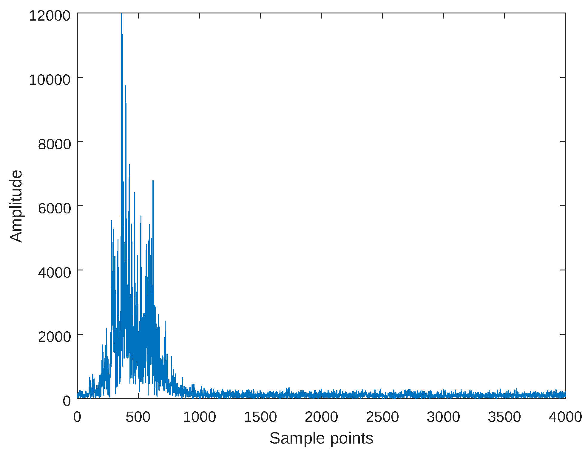
| Number of samples per chirp | 4000 | |
| Number of chirps | 1 |
Disclaimer/Publisher’s Note: The statements, opinions and data contained in all publications are solely those of the individual author(s) and contributor(s) and not of MDPI and/or the editor(s). MDPI and/or the editor(s) disclaim responsibility for any injury to people or property resulting from any ideas, methods, instructions or products referred to in the content. |
© 2025 by the authors. Licensee MDPI, Basel, Switzerland. This article is an open access article distributed under the terms and conditions of the Creative Commons Attribution (CC BY) license (https://creativecommons.org/licenses/by/4.0/).
Share and Cite
Huang, Z.; Jiang, P.; Fu, M.; Deng, Z. Angle Estimation for Range-Spread Targets Based on Scatterer Energy Focusing. Sensors 2025, 25, 1723. https://doi.org/10.3390/s25061723
Huang Z, Jiang P, Fu M, Deng Z. Angle Estimation for Range-Spread Targets Based on Scatterer Energy Focusing. Sensors. 2025; 25(6):1723. https://doi.org/10.3390/s25061723
Chicago/Turabian StyleHuang, Zekai, Peiwu Jiang, Maozhong Fu, and Zhenmiao Deng. 2025. "Angle Estimation for Range-Spread Targets Based on Scatterer Energy Focusing" Sensors 25, no. 6: 1723. https://doi.org/10.3390/s25061723
APA StyleHuang, Z., Jiang, P., Fu, M., & Deng, Z. (2025). Angle Estimation for Range-Spread Targets Based on Scatterer Energy Focusing. Sensors, 25(6), 1723. https://doi.org/10.3390/s25061723