
Mission Sequence Model and Deep Reinforcement Learning-Based Replanning Method for Multi-Satellite Observation

Abstract
1. Introduction
- To the best of our knowledge, this is the first work to directly model satellite observation sequences using deep learning, incorporating time and attitude information. We utilize task timing and side-swing angles as positional encodings for self-attention modeling and introduce a gated global pooling method based on interval information to generate a comprehensive satellite state representation. Ablation studies and comparisons with classical methods demonstrate that our approach significantly improves mission replanning performance.
- We propose a DRL-based mission replanning algorithm for a single satellite, designed to handle discrete-continuous hybrid decision variables. This algorithm achieves dual-objective optimization by maximizing task revenues and minimizing changes to the original plan. Experimental results validate the effectiveness of the algorithm, demonstrating its generalization ability across different-scale scenarios.
- We propose an on-site mission allocation algorithm for request-receiving satellites, integrating cross-attention mechanisms and pointer networks to provide end-to-end allocation solutions. Combined with the replanning method, this two-stage optimization approach demonstrates the advantages of our algorithm over classical methods.
2. Literature Review
2.1. Dynamic Scheduling of AEOSs
2.2. Multi-Satellite Scheduling Architecture
2.3. General Models and Algorithms
3. Problem Statement
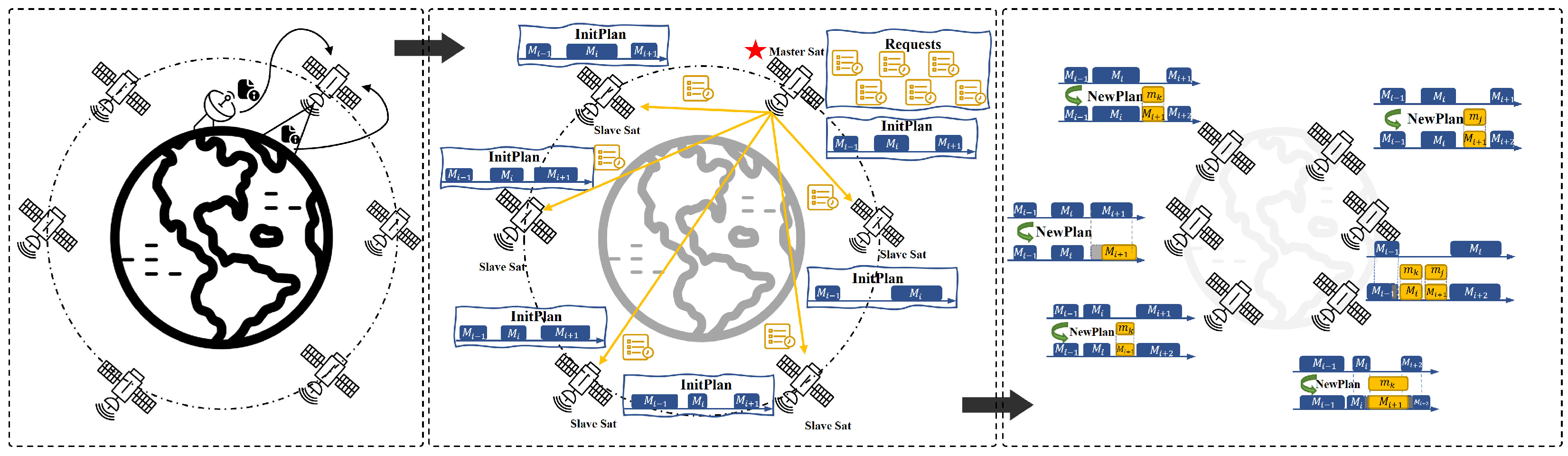
3.1. Scenario and Replanning Framework
3.2. Assumptions and Definitions
- Assuming that a group of satellites . Each satellite is represented as , where are static parameters that remain constant during the scheduling process. These parameters, which reflect inherent task characteristics, are pre-determined and include the attitude transition rate (), maximum side swing angle (), memory capacity (), and power capacity (). Conversely, are dynamic parameters, which are updated at each scheduling step to represent the current side swing angle (), remaining memory (), and remaining power () at any given time. It is important to note that, in our model, operates continuously on orbit and does not perform any orbit-raising maneuvers.
- Dynamic requests can be represented as . Each request is defined as . It contains a quadruple, are the start time and end time of the visible time window of to request ; is the execution duration required for ; represents the side swing angle required for observation to . Additionally, the request includes the priority , required memory consumption , and required power consumption .
- When a request is scheduled into the mission sequence of a designated satellite , it is represented as , where represent the start and end time of the mission execution, and indicates the reward associated with the task. Each satellite has an optimal initial plan , that contains missions; The updated mission plan is represented as , with a length of .
- We define that new requests arrive in batches, and at each time step, only one satellite will be designated as the master satellite for task allocation.
- The integration of new requests into the mission sequence must satisfy the constraints of the satellite imaging tasks.
3.3. Objective Function and Constraints
- Visible Time Window Constraint: The start and end of the execution time in the satellite’s mission sequence must satisfy
- Transition Time Constraint: Continuous missions must satisfy the attitude transition requirement. After completion of the previous task , the satellite must undergo a specified maneuver, ensuring that can still complete the observation before the end of its visible time window.
- Adjustment Time Range Constraint: The time window within which can be moved is determined by its visible time window , as well as the execution times of the preceding task and the following task . The maximum advancement time isThe maximum delay time is
- Uniqueness constraints: Each request has a different visible time window for each satellite, but it can only be executed by one satellite at a time.Each task can only be observed once. For any given satellite, each selected task can have at most one preceding task and one succeeding task.
- Resource Constraint: The complete is managed through the removal of resource-exceeding tasks from its terminal end.
4. Solution Method
| Algorithm 1 The framework of MSRP |
| Input: Satellite set , Request set arrive at , original plan Output: New plan Enhance State Representation: Mission Allocation in : for do Select through Assign to end for return for each /*proceed in parallel*/ Mission Replanning in : while not terminated do Get though Insert into end while Output Optimal Scheme |
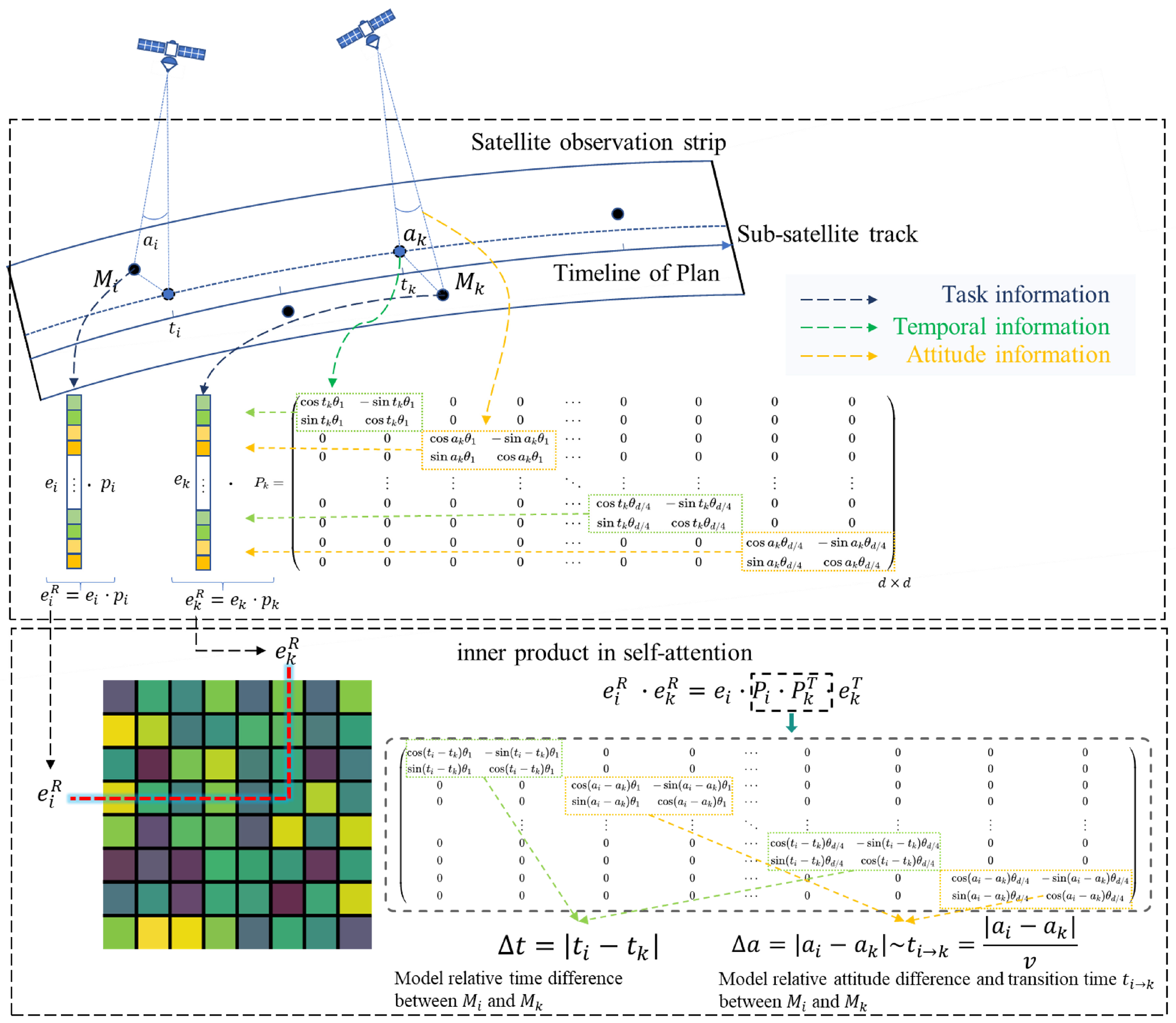
4.1. Mission Sequence Modeling
4.2. Dynamic Request Modeling
4.3. Multi-Satellite Mission Allocation
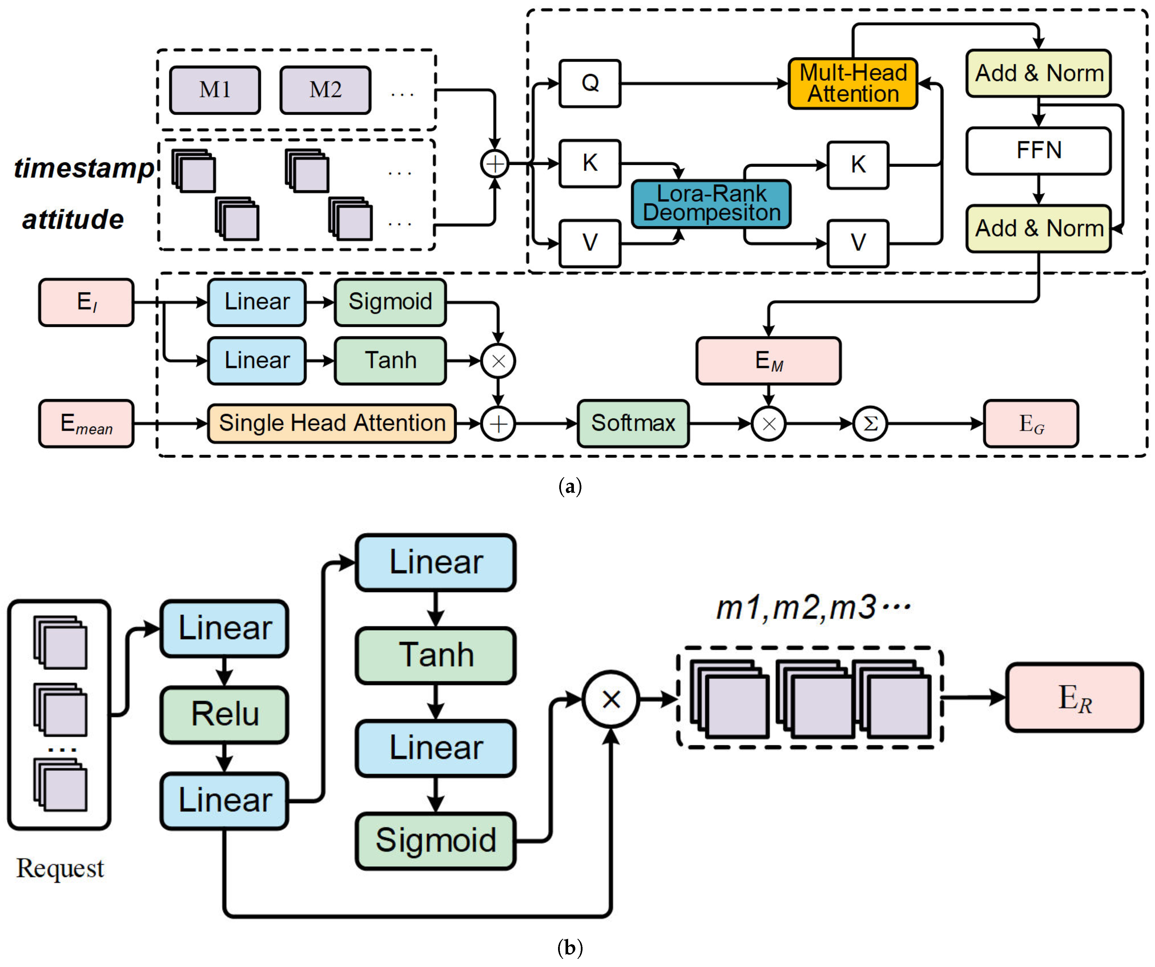
- State: In mission allocation, the state at step t comprises two parts: the mission sequence of satellites from and the dynamic request set. The satellites’ immediate state and resource changes are recorded within schedule. Using the mission sequence modeling method, we derive satellites’ global embedding . For dynamic requests, we generate the global embedding and individual request vectors as .
- Action: The action space consists of satellites awaiting task allocation, defined as a discrete set. We employ a pointer mechanism to generate the policy function, with the detailed procedure outlined in the following steps and visually represented in Figure 4a.
- (a)
- Apply a cross-attention layer, where the query is the satellite state , and the key and value are the requests . The output is the mission-satellite association vector , which aims to capture the relationships between the satellite and all requests.
- (b)
- Concatenating each request vector with global embedding to construct vector .
- (c)
- We use a pointer mechanism to generate the probability distribution of the allocation policy .
- Reward: The objective of mission allocation is to maximize the overall reward, which is determined after replanning by each satellite. Therefore, mission allocation is jointly optimized with the single-satellite replanning algorithm. If a request is successfully inserted into the plan, the step reward is the task’s revenue; otherwise, it returns zero. The revenue of each request is normalized by the sum of total revenues.
4.4. Single-Satellite Mission Replanning
- State: In this replanning phase, the satellite state is represented by its mission sequence embedding , which incorporates resource consumption. The global state is given by the pooling method. The dynamically arriving requests, with an uncertain scale , are encoded and represented as .
- Action: The replanning actions are composite, using a hybrid action space. Each action at step t is represented as where denotes the task selected from the allocated set, and refers to the execution time of the selected task. We introduce a termination action to end the replanning process. The action generation is handled by two branches of the actor network, which output discrete and continuous actions, respectively. The specific actor network is illustrated in Figure 4b.
- (a)
- State Extraction: Two consecutive cross-attention blocks are used to build a compressed representation of the current state. In the first block, , which generates the task-satellite affinity vector . In the second block, , where the satellite’s global state is used as the query to capture the current global state .
- (b)
- Discrete Action: The mission selection policy distribution is generated using the pointer mechanism.
- (c)
- Continuous Action: Add the selected task information into the actor network to generate the mean , and variance . After sampling from , we scale the action to the range using the Tanh function. The output is then re-normalized to the specific mission’s start time using the formula.
- (d)
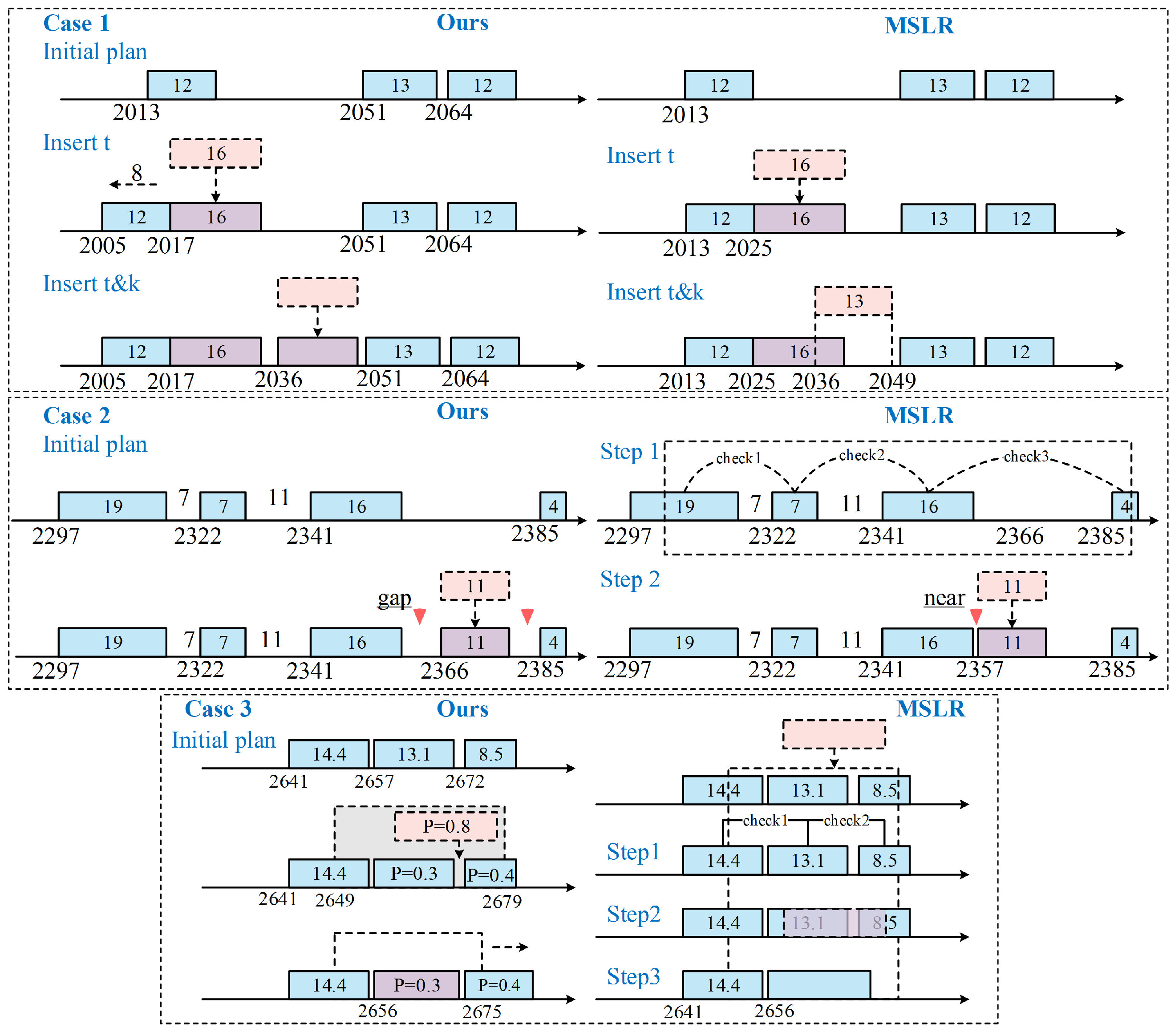
- Mission Insertion: The mission is inserted based on . In case of conflicts with existing missions, a fast insertion approach (FIA) like principle [19] is applied to resolve the conflict by shifting existing task or removing it if necessary.
- Reward: Our optimization objective consists of two parts: mission revenues and the cost function associated with changes to the initial mission sequence. Thus, we design the reward as follows:where are adjustable parameters that satisfy . represents the length of the satellite mission sequence at step t, denotes the revenue of , and is the penalty factor for different levels of modifications. The goal of our reward design is to maximize both the task plan length and revenues while minimizing the disruption to the original plan during urgent request scheduling.
4.5. Training
| Algorithm 2 Procedure for training policy based on PPO |
|
5. Computational Experiments
5.1. Scenario Settings
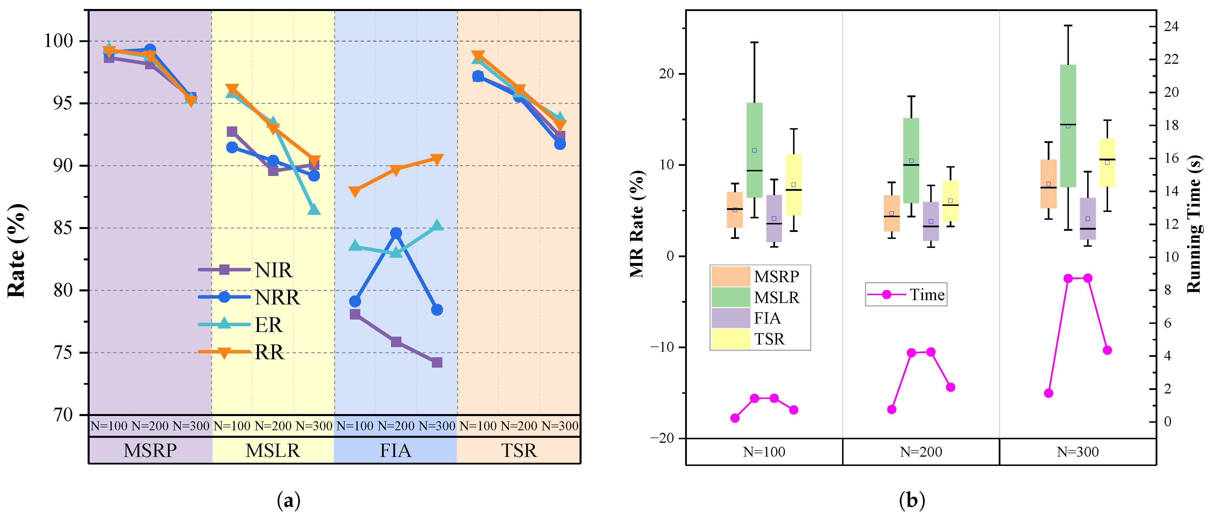
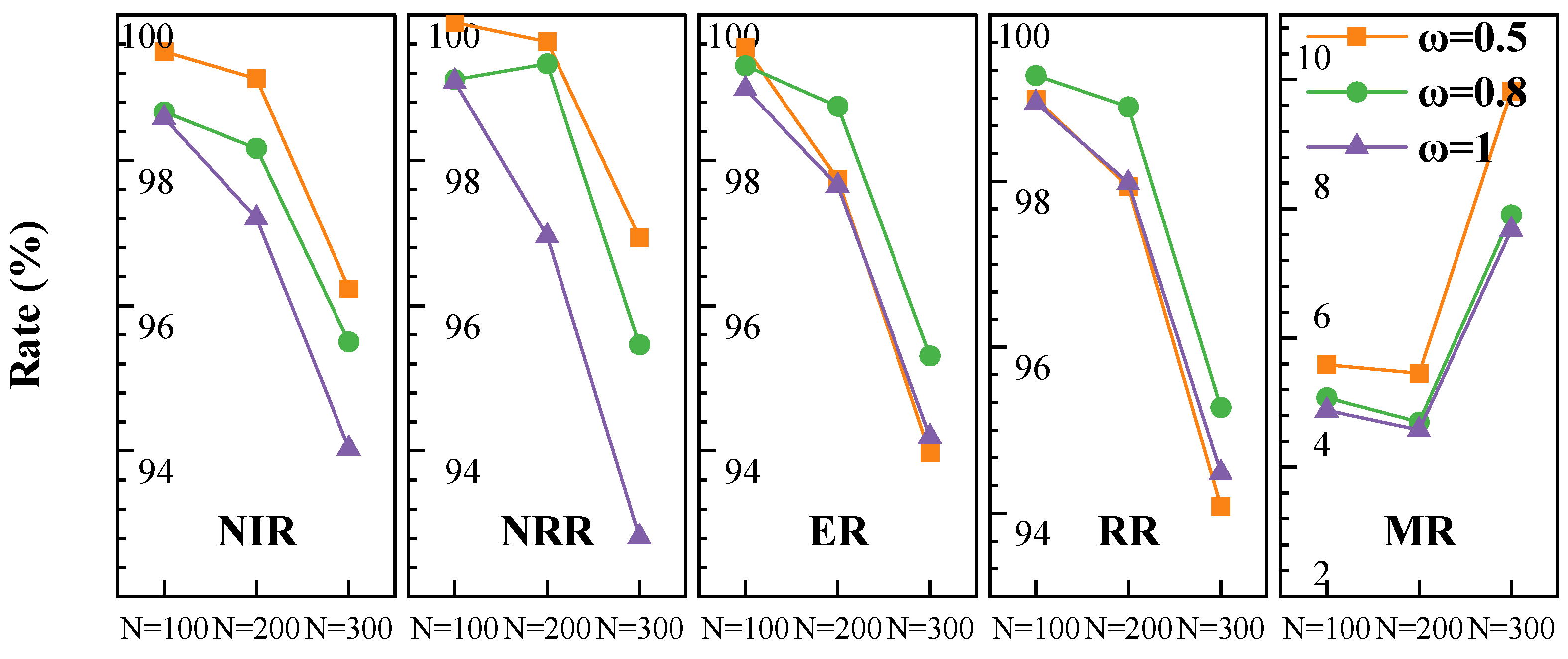
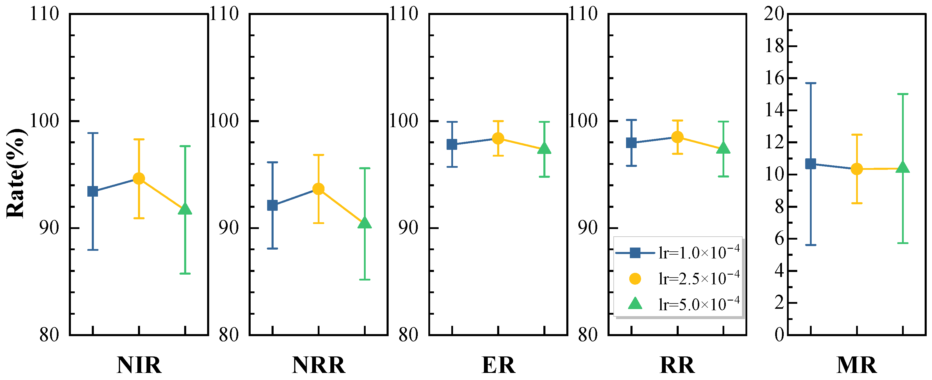
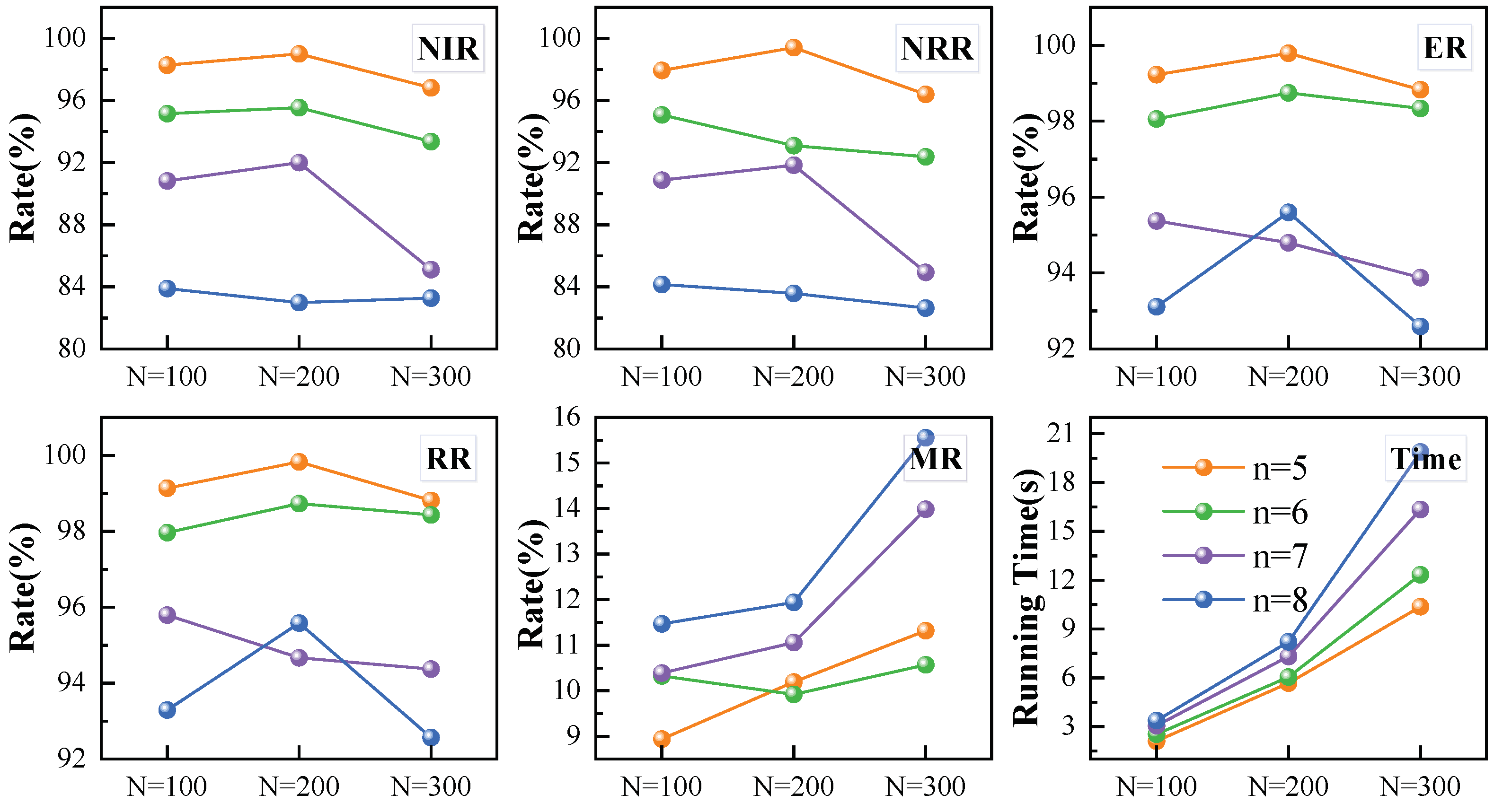
- Insert rate of new requests: ;
- Revenue rate of new request: ;
- Execution rate of missions: ;
- Total Revenue rate: ;
- Modification rate: ;
- Computation time: .
5.2. Comparison Algorithms
- Multiple Strategies Local Replanning (MSLR) Algorithm: This algorithm integrates multiple insertion principles from [66]: direct insertion, move insertion, replace insertion; along with a hybrid insertion strategy from [7]: direct insertion, iterative insertion, conflict replacement insertion. Since our scenario focuses on mission-satellite visible time windows, we combined the merging insertion into direct insertion.
- Transformer-based single-satellite replanning (TSR) Algorithm: We adopt the Transformer-based architecture with temporal encoding from [62] as the task scheduling method for single-satellite replanning. After obtaining discrete decisions, we use a neural network with the same architecture as MSRP to compute continuous actions.
- Fast Insertion Approach (FIA) Algorithm: Based on the FIA principles from [19], this approach prioritizes tasks and determines insertion positions based on their feasibility between adjacent tasks in the satellite sequence, optimizing overall gain.
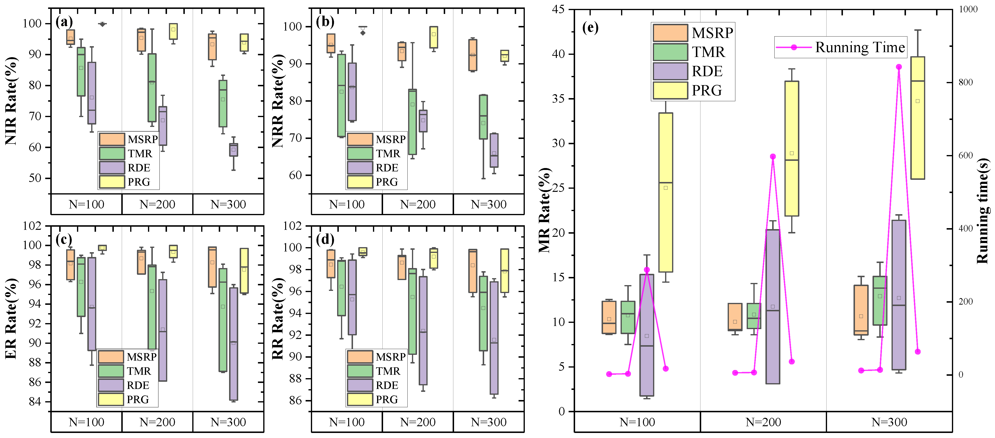
- Transformer-based multi-satellite replanning (TMR) Algorithm: We combine the multi-satellite task allocation framework based on the attention mechanism from [67] with TSR as the single-satellite replanning method, forming our comparative algorithm.
- Plan Regenerate (PRG) method: Based on the ADSMP method, we regenerate the task sequence by inputting both dynamic requests and the original missions.
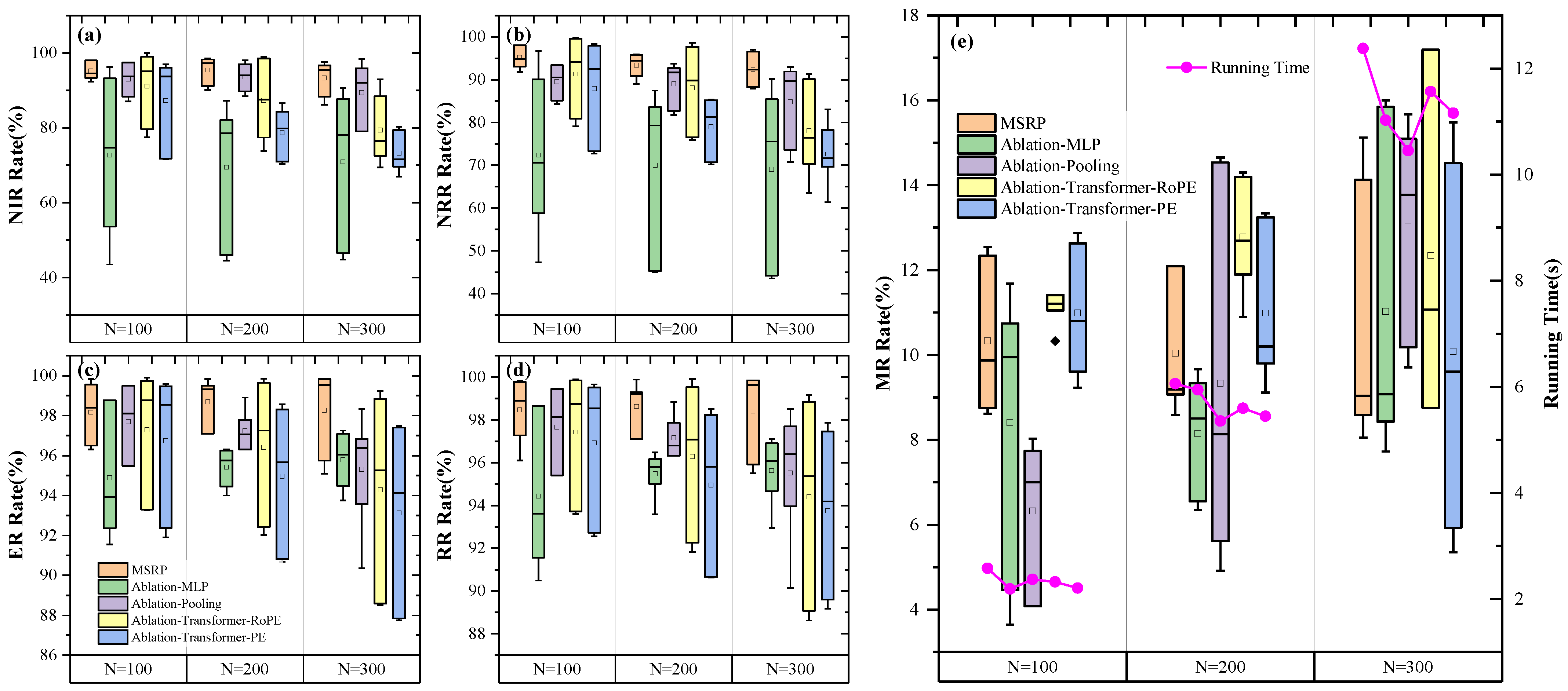
- Ablation-MLP: To validate the effectiveness of our mission sequence modeling module, we developed a baseline embedding network for comparison, represented by a three-layer MLP with 128 nodes. This network processes satellite mission sequence information and matches the input for the subsequent policy network. We used the PPO algorithm for training.
- Ablation-pooling: To verify the effectiveness of our global pooling module, we replaced it with a mean pooling method for ablation. The PPO algorithm was used to train this version.
- Ablation-Transformer-PE: Replace mission sequence modeling method by standard attention with classic position encoding (PE) for ablation.
- Ablation-Transformer-RoPE: Replace mission sequence modeling method by standard attention with Rotary Position Embedding (RoPE) for ablation.
5.3. Experiment 1 on Single-Satellite Replanning
5.4. Experiment 2 on Multi-Satellite Replanning Framework
5.5. Experiment 3 for Ablation
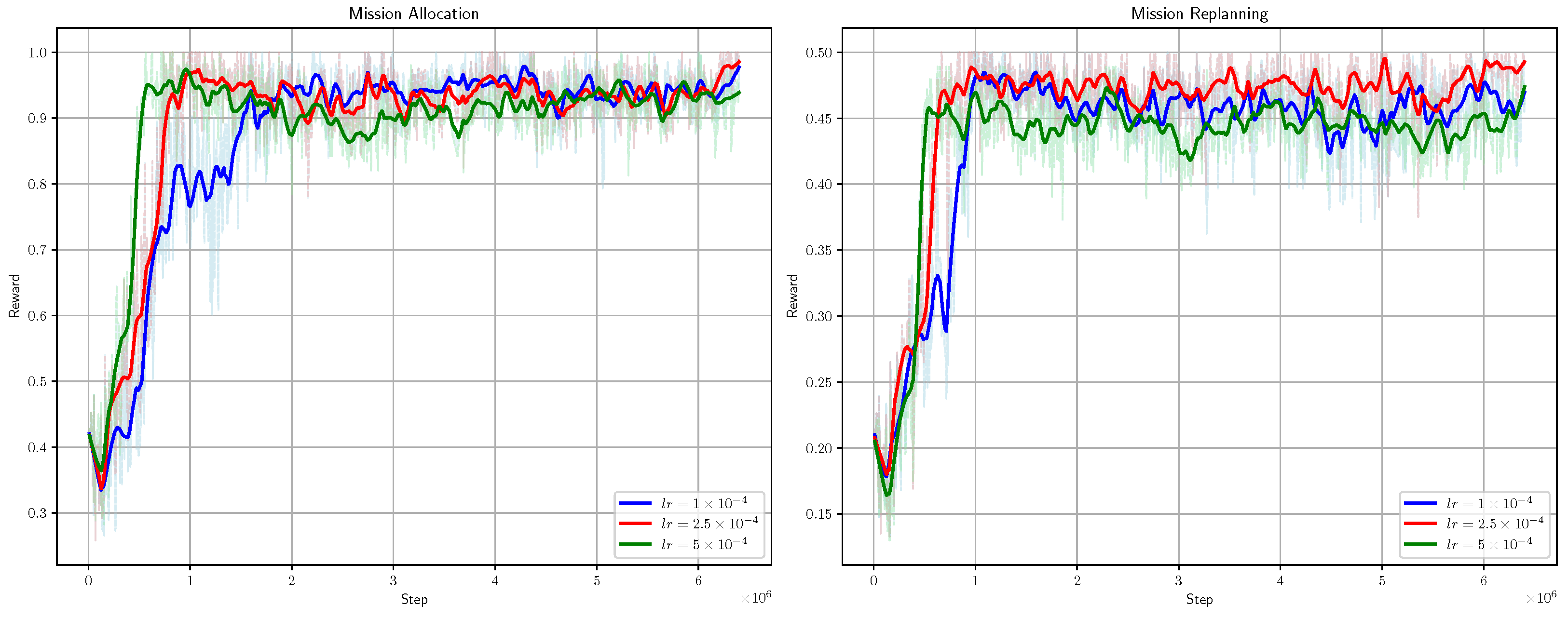
5.6. Sensitivity Analysis
6. Conclusions
Author Contributions
Funding
Institutional Review Board Statement
Informed Consent Statement
Data Availability Statement
Conflicts of Interest
References
- Lemaître, M.; Verfaillie, G.; Jouhaud, F.; Lachiver, J.; Bataille, N. Selecting and scheduling observations of agile satellites. Aerosp. Sci. Technol. 2002, 6, 367–381. [Google Scholar] [CrossRef]
- Crisp, N.H.; Roberts, P.C.E.; Livadiotti, S.; Oiko, V.T.A.; Edmondson, S.; Haigh, S.J.; Huyton, C.; Sinpetru, L.A.; Smith, K.L.; Worrall, S.D.; et al. The benefits of very low earth orbit for earth observation missions. Prog. Aerosp. Sci. 2020, 117, 100619. [Google Scholar] [CrossRef]
- Zheng, Z. Autonomous Onboard Mission Planning for Multiple Satellite Systems. Ph.D. Thesis, Delft University of Technology, Delft, The Netherlands, 2019. [Google Scholar] [CrossRef]
- Cui, J.; Zhang, X. Application of a Multi-Satellite Dynamic Mission Scheduling Model Based on Mission Priority in Emergency Response. Sensors 2019, 19, 1430. [Google Scholar] [CrossRef] [PubMed]
- Lu, Z.; Shen, X.; Li, D.; Cheng, S.; Wang, J.; Yao, W. Super-agile satellites imaging mission planning method considering degradation of image MTF in dynamic imaging. Int. J. Appl. Earth Obs. Geoinf. 2024, 131, 103968. [Google Scholar] [CrossRef]
- Xiao, Y.; Zhang, S.; Yang, P.; You, M.; Huang, J. A two-stage flow-shop scheme for the multi-satellite observation and data downlink scheduling problem considering weather uncertainties. Reliab. Eng. Syst. Saf. 2019, 188, 263–275. [Google Scholar] [CrossRef]
- Yang, X.; Hu, M.; Huang, G.; Li, A. A Hybrid Local Replanning Strategy for Multi-Satellite Imaging Mission Planning in Uncertain Environments. IEEE Access 2023, 11, 120780–120804. [Google Scholar] [CrossRef]
- Wang, J.; Zhu, X.; Qiu, D.; Yang, L.T. Dynamic Scheduling for Emergency Tasks on Distributed Imaging Satellites with Task Merging. IEEE Trans. Parallel Distrib. Syst. 2014, 25, 2275–2285. [Google Scholar] [CrossRef]
- Chong, W.; Jun, L.; Ning, J.; Jun, W.; Hao, C. A Distributed Cooperative Dynamic Task Planning Algorithm for Multiple Satellites Based on Multi-agent Hybrid Learning. Chin. J. Aeronaut. 2011, 24, 493–505. [Google Scholar] [CrossRef]
- Li, H.; Li, Y.; Liu, Y.; Zhang, K.; Li, X.; Li, Y.; Zhao, S. A Multi-Objective Dynamic Mission-Scheduling Algorithm Considering Perturbations for Earth Observation Satellites. Aerospace 2024, 11, 643. [Google Scholar] [CrossRef]
- Yang, Y.; Liu, D. Distributed Imaging Satellite Mission Planning Based on Multi-Agent. IEEE Access 2023, 11, 65530–65545. [Google Scholar] [CrossRef]
- Sun, H.; Xia, W.; Hu, X.; Xu, C. Earth observation satellite scheduling for emergency tasks. J. Syst. Eng. Electron. 2019, 30, 931–945. [Google Scholar] [CrossRef]
- He, L.; Liu, X.L.; Chen, Y.W.; Xing, L.N.; Liu, K. Hierarchical scheduling for real-time agile satellite task scheduling in a dynamic environment. Adv. Space Res. 2019, 63, 897–912. [Google Scholar] [CrossRef]
- Li, H.; Li, Y.; Meng, Q.Q.; Li, X.; Shao, L.; Zhao, S. An onboard periodic rescheduling algorithm for satellite observation scheduling problem with common dynamic tasks. Adv. Space Res. 2024, 73, 5242–5253. [Google Scholar] [CrossRef]
- Li, K.; Zhang, T.; Wang, R. Deep Reinforcement Learning for Multiobjective Optimization. IEEE Trans. Cybern. 2021, 51, 3103–3114. [Google Scholar] [CrossRef] [PubMed]
- Pemberton, J.C.; Greenwald, L. On the need for dynamic scheduling of imaging satellites. Int. Arch. Photogramm. Remote Sens. Spat. Inf. Sci. 2002, 34, 165–171. [Google Scholar]
- Liang, J.; Zhu, Y.H.; Luo, Y.Z.; Zhang, J.C.; Zhu, H. A precedence-rule-based heuristic for satellite onboard activity planning. Acta Astronaut. 2021, 178, 757–772. [Google Scholar] [CrossRef]
- Wen, J.; Liu, X.; He, L. Real-time online rescheduling for multiple agile satellites with emergent tasks. J. Syst. Eng. Electron. 2021, 32, 1407–1420. [Google Scholar] [CrossRef]
- Han, C.; Gu, Y.; Wu, G.; Wang, X. Simulated Annealing-Based Heuristic for Multiple Agile Satellites Scheduling Under Cloud Coverage Uncertainty. IEEE Trans. Syst. Man Cybern.-Syst. 2023, 53, 2863–2874. [Google Scholar] [CrossRef]
- Liu, S.; Chen, Y.; Xing, L.; Guo, X. Time-dependent autonomous task planning of agile imaging satellites. J. Intell. Fuzzy Syst. 2016, 31, 1365–1375. [Google Scholar] [CrossRef]
- Wei, L.; Xing, L.; Wan, Q.; Song, Y.; Chen, Y. A Multi-objective Memetic Approach for Time-dependent Agile Earth Observation Satellite Scheduling Problem. Comput. Ind. Eng. 2021, 159, 107530. [Google Scholar] [CrossRef]
- Peng, G.; Song, G.; He, Y.; Yu, J.; Xiang, S.; Xing, L.; Vansteenwegen, P. Solving the Agile Earth Observation Satellite Scheduling Problem With Time-Dependent Transition Times. IEEE Trans. Syst. Man Cybern.-Syst. 2022, 52, 1614–1625. [Google Scholar] [CrossRef]
- Du, B.; Li, S. A new multi-satellite autonomous mission allocation and planning method. Acta Astronaut. 2019, 163, 287–298. [Google Scholar] [CrossRef]
- Du, Y.; Wang, T.; Xin, B.; Wang, L.; Chen, Y.; Xing, L. A Data-Driven Parallel Scheduling Approach for Multiple Agile Earth Observation Satellites. IEEE Trans. Evol. Comput. 2020, 24, 679–693. [Google Scholar] [CrossRef]
- Song, Y.; Xing, L.; Wang, M.; Yi, Y.; Xiang, W.; Zhang, Z. A knowledge-based evolutionary algorithm for relay satellite system mission scheduling problem. Comput. Ind. Eng. 2020, 150, 106830. [Google Scholar] [CrossRef]
- Zhu, W.; Hu, X.; Xia, W.; Jin, P. A two-phase genetic annealing method for integrated Earth observation satellite scheduling problems. Soft Comput. 2019, 23, 181–196. [Google Scholar] [CrossRef]
- Wang, Y.; Liu, D.; Liu, J. A Bilevel Programming Model for Multi-Satellite Cooperative Observation Mission Planning. IEEE Access 2024, 12, 145439–145449. [Google Scholar] [CrossRef]
- Bianchessi, N.; Cordeau, J.F.; Desrosiers, J.; Laporte, G.; Raymond, V. A heuristic for the multi-satellite, multi-orbit and multi-user management of Earth observation satellites. Eur. J. Oper. Res. 2007, 177, 750–762. [Google Scholar] [CrossRef]
- Li, J.; Chen, Y.; Liu, X.; He, R. JADE implemented multi-agent based platform for multiple autonomous satellite system. In Proceedings of the 2018 SpaceOps Conference, Marseille, France, 28 May–1 June 2018; p. 2349. [Google Scholar] [CrossRef]
- Qi, J.; Guo, J.; Wang, M.; Wu, C. A Cooperative Autonomous Scheduling Approach for Multiple Earth Observation Satellites With Intensive Missions. IEEE Access 2021, 9, 61646–61661. [Google Scholar] [CrossRef]
- Liu, Y.; Chen, Q.; Li, C.; Wang, F. Mission planning for Earth observation satellite with competitive learning strategy. Aerosp. Sci. Technol. 2021, 118, 107047. [Google Scholar] [CrossRef]
- Chen, Y.; Tian, G.; Guo, J.; Huang, J. Task Planning for Multiple-Satellite Space-Situational-Awareness Systems. Aerospace 2021, 8, 73. [Google Scholar] [CrossRef]
- Yang, W.; He, L.; Liu, X.; Chen, Y. Onboard coordination and scheduling of multiple autonomous satellites in an uncertain environment. Adv. Space Res. 2021, 68, 4505–4524. [Google Scholar] [CrossRef]
- Li, J.; Yang, A.; Jing, N.; Hu, W. Coordinated planning of space-aeronautics earth-observing based on CSP theory. In Proceedings of the 2013 21st International Conference on Geoinformatics, Kaifeng, China, 20–22 June 2013. [Google Scholar] [CrossRef]
- Liu, D.; Dou, L.; Zhang, R.; Zhang, X.; Zong, Q. Multi-Agent Reinforcement Learning-Based Coordinated Dynamic Task Allocation for Heterogenous UAVs. IEEE Trans. Veh. Technol. 2023, 72, 4372–4383. [Google Scholar] [CrossRef]
- Dalin, L.; Haijiao, W.; Zhen, Y.; Yanfeng, G.; Shi, S. An Online Distributed Satellite Cooperative Observation Scheduling Algorithm Based on Multiagent Deep Reinforcement Learning. IEEE Geosci. Remote Sens. Lett. 2021, 18, 1901–1905. [Google Scholar] [CrossRef]
- Saeed, A.K.; Holguin, F.; Yasin, A.S.; Johnson, B.A.; Rodriguez, B.M. Multi-Agent and Multi-Target Reinforcement Learning for Satellite Sensor Tasking. In Proceedings of the 2024 IEEE Aerospace Conference, Big Sky, MT, USA, 2–9 March 2024; pp. 1–13. [Google Scholar] [CrossRef]
- Zhang, G.; Li, X.; Hu, G.; Li, Y.; Wang, X.; Zhang, Z. MARL-Based Multi-Satellite Intelligent Task Planning Method. IEEE Access 2023, 11, 135517–135528. [Google Scholar] [CrossRef]
- Xhafa, F.; Ip, A.W. Optimisation problems and resolution methods in satellite scheduling and space-craft operation: A survey. Enterp. Inf. Syst. 2021, 15, 1022–1045. [Google Scholar] [CrossRef]
- Cho, D.H.; Kim, J.H.; Choi, H.L.; Ahn, J. Optimization-Based Scheduling Method for Agile Earth-Observing Satellite Constellation. J. Aerosp. Inf. Syst. 2018, 15, 611–626. [Google Scholar] [CrossRef]
- Kim, J.; Ahn, J.; Choi, H.L.; Cho, D.H. Task Scheduling of Agile Satellites with Transition Time and Stereoscopic Imaging Constraints. J. Aerosp. Inf. Syst. 2020, 17, 285–293. [Google Scholar] [CrossRef]
- Li, P.; Li, J.; Li, H.; Zhang, S.; Yang, G. Graph Based Task Scheduling Algorithm for Earth Observation Satellites. In Proceedings of the 2018 IEEE Global Communications Conference (GLOBECOM), Abu Dhabi, United Arab Emirates, 9–13 December 2018; pp. 1–7. [Google Scholar] [CrossRef]
- Gabrel, V.; Moulet, A.; Murat, C.; Paschos, V.T. A new single model and derived algorithms for the satellite shot planning problem using graph theory concepts. Ann. Oper. Res. 1997, 69, 115–134. [Google Scholar] [CrossRef]
- Valicka, C.G.; Garcia, D.; Staid, A.; Watson, J.P.; Hackebeil, G.; Rathinam, S.; Ntaimo, L. Mixed-integer programming models for optimal constellation scheduling given cloud cover uncertainty. Eur. J. Oper. Res. 2019, 275, 431–445. [Google Scholar] [CrossRef]
- Song, Y.; Xing, L.; Chen, Y. Two-stage hybrid planning method for multi-satellite joint observation planning problem considering task splitting. Comput. Ind. Eng. 2022, 174, 108795. [Google Scholar] [CrossRef]
- Chen, Y.; Lu, J.; He, R.; Ou, J. An Efficient Local Search Heuristic for Earth Observation Satellite Integrated Scheduling. Appl. Sci. 2020, 10, 5616. [Google Scholar] [CrossRef]
- Luo, Q.; Peng, W.; Wu, G.; Xiao, Y. Orbital Maneuver Optimization of Earth Observation Satellites Using an Adaptive Differential Evolution Algorithm. Remote Sens. 2022, 14, 1966. [Google Scholar] [CrossRef]
- Li, Y.; Luo, J.; Zhang, W.; Xiang, F. Genetic-evolutionary bi-level mission planning algorithm for multi-satellite cooperative observation. Syst. Eng. Electron. 2024, 46, 2044. [Google Scholar]
- Zheng, Z.; Guo, J.; Gill, E. Onboard autonomous mission re-planning for multi-satellite system. Acta Astronaut. 2018, 145, 28–43. [Google Scholar] [CrossRef]
- Mao, H.; Alizadeh, M.; Menache, I.; Kandula, S. Resource Management with Deep Reinforcement Learning. In Proceedings of the 15th ACM Workshop on Hot Topics in Networks, Atlanta GA USA, 9–10 November 2016; Association for Computing Machinery: New York, NY, USA, 2016. HotNets ’16. pp. 50–56. [Google Scholar] [CrossRef]
- Chen, H.; Luo, Z.; Peng, S.; Wu, J.; Li, J. HiPGen: An approach for fast generation of multi-satellite observation plans via a hierarchical multi-channel transformer network. Adv. Space Res. 2022, 69, 3103–3116. [Google Scholar] [CrossRef]
- Gu, Y.; Han, C.; Chen, Y.; Xing, W.W. Mission Replanning for Multiple Agile Earth Observation Satellites Based on Cloud Coverage Forecasting. IEEE J. Sel. Top. Appl. Earth Obs. Remote Sens. 2022, 15, 594–608. [Google Scholar] [CrossRef]
- Wang, H.; Yang, Z.; Zhou, W.; Li, D. Online scheduling of image satellites based on neural networks and deep reinforcement learning. Chin. J. Aeronaut. 2019, 32, 1011–1019. [Google Scholar] [CrossRef]
- Schuetz, M.J.; Brubaker, J.K.; Katzgraber, H.G. Combinatorial optimization with physics-inspired graph neural networks. Nat. Mach. Intell. 2022, 4, 367–377. [Google Scholar] [CrossRef]
- Wang, Z.; Hu, X.; Ma, H.; Xia, W. Learning multi-satellite scheduling policy with heterogeneous graph neural network. Adv. Space Res. 2024, 73, 2921–2938. [Google Scholar] [CrossRef]
- Feng, X.; Li, Y.; Xu, M. Multi-satellite cooperative scheduling method for large-scale tasks based on hybrid graph neural network and metaheuristic algorithm. Adv. Eng. Inform. 2024, 60, 102362. [Google Scholar] [CrossRef]
- Nazari, M.; Oroojlooy, A.; Takáč, M.; Snyder, L.V. Reinforcement learning for solving the vehicle routing problem. In Proceedings of the 32nd International Conference on Neural Information Processing Systems, Montréal, QC, Canada, 3–8 December 2018; Curran Associates Inc.: Red Hook, NY, USA, 2018. NIPS’18. pp. 9861–9871. [Google Scholar]
- Kool, W.; van Hoof, H.; Welling, M. Attention, Learn to Solve Routing Problems! In Proceedings of the International Conference on Learning Representations, New Orleans, LA, USA, 6–9 May 2019.
- Liu, Z.; Xiong, W.; Han, C.; Yu, X. Deep Reinforcement Learning with Local Attention for Single Agile Optical Satellite Scheduling Problem. Sensors 2024, 24, 6396. [Google Scholar] [CrossRef]
- Chen, M.; Du, Y.; Tang, K.; Xing, L.; Chen, Y.; Chen, Y. Learning to Construct a Solution for the Agile Satellite Scheduling Problem With Time-Dependent Transition Times. IEEE Trans. Syst. Man Cybern. Syst. 2024, 54, 5949–5963. [Google Scholar] [CrossRef]
- Liang, J.; Liu, J.P.; Sun, Q.; Zhu, Y.H.; Zhang, Y.C.; Song, J.G.; He, B.Y. A Fast Approach to Satellite Range Rescheduling Using Deep Reinforcement Learning. IEEE Trans. Aerosp. Electron. Syst. 2023, 59, 9390–9403. [Google Scholar] [CrossRef]
- Long, Y.; Shan, C.; Shang, W.; Li, J.; Wang, Y. Deep Reinforcement Learning-Based Approach With Varying-Scale Generalization for the Earth Observation Satellite Scheduling Problem Considering Resource Consumptions and Supplements. IEEE Trans. Aerosp. Electron. Syst. 2024, 60, 2572–2585. [Google Scholar] [CrossRef]
- Jiang, Y.; Yang, Y.; Xu, Y.; Wang, E. Spatial-Temporal Interval Aware Individual Future Trajectory Prediction. IEEE Trans. Knowl. Data Eng. 2024, 36, 5374–5387. [Google Scholar] [CrossRef]
- Agrawal, A.; Bedi, A.S.; Manocha, D. RTAW: An Attention Inspired Reinforcement Learning Method for Multi-Robot Task Allocation in Warehouse Environments. In Proceedings of the 2023 IEEE International Conference on Robotics and Automation (ICRA), London, UK, 29 May–2 June 2023; pp. 1393–1399. [Google Scholar] [CrossRef]
- Li, P.; Wang, H.; Zhang, Y.; Pan, R. Mission planning for distributed multiple agile Earth observing satellites by attention-based deep reinforcement learning method. Adv. Space Res. 2024, 74, 2388–2404. [Google Scholar] [CrossRef]
- Sun, H.; Xia, W.; Wang, Z.; Hu, X. Agile earth observation satellite scheduling algorithm for emergency tasks based on multiple strategies. J. Syst. Sci. Syst. Eng. 2021, 30, 626–646. [Google Scholar] [CrossRef]
- Ou, J.; Xing, L.; Yao, F.; Li, M.; Lv, J.; He, Y.; Song, Y.; Wu, J.; Zhang, G. Deep reinforcement learning method for satellite range scheduling problem. Swarm Evol. Comput. 2023, 77, 101233. [Google Scholar] [CrossRef]


| Satellite | a (km) | e | I (°) | (°) | (°) | M (°) |
|---|---|---|---|---|---|---|
| Sat1 | 7200.0 | 0.000627 | 96.5760 | 0 | 175.72 | 0.0750 |
| Sat2 | 7200.0 | 0.000627 | 96.5760 | 0 | 145.72 | 30.0750 |
| Sat3 | 7200.0 | 0.000627 | 96.5760 | 0 | 115.72 | 60.0750 |
| Sat4 | 7200.0 | 0.000627 | 96.5760 | 0 | 85.72 | 90.0750 |
| Sat5 | 7200.0 | 0.000627 | 96.5760 | 0 | 55.72 | 120.0750 |
| Sat6 | 7200.0 | 0.000627 | 96.5760 | 0 | 25.72 | 150.0750 |
| Parameters | Value | Unit | Description |
|---|---|---|---|
| s | Required execution duration | ||
| [0.1, 0.9] | 1 | Revenue (priority) of request | |
| [−50, 50] | 1 | Side swing angle range | |
| 1000 | GB | Memory capacity | |
| GB | Memory consumption | ||
| 512 | W· h | Power capacity | |
| W· h | Power consumption | ||
| 1 | s/deg | Time per degree of transition |
| Hyperparameters | Replanning | Allocation |
|---|---|---|
| Number of envs | 128 | 32 |
| Total timesteps | 64 × 105 | 64 × 105 |
| Mini-batches | 32 | 8 |
| Learning rate | 2.5 × 10⁻⁴ | 2.5 × 10⁻⁴ |
| Learning rate decay | CosineAnnealing | StepAnnealing |
| 0.99 | 0.99 | |
| GAE | 0.95 | 0.95 |
| Update epochs | 8 | 4 |
| Cliping coefficient | 0.2 | 0.1 |
| Entropy coefficiant | 0.01 | 0.01 |
| Embedding dimension | 128 | 128 |
| Gate embedding dimension | 32 | 32 |
| Algorithm Comparison | Statistical Indicators | NIR | NRR | ER | RR | MR | Time | Significant Difference (y/n) |
|---|---|---|---|---|---|---|---|---|
| MSRP|MSLR | Wilcoxon signed ranks test p-value | 0.0033 | 0.0033 | 0.0033 | 0.0033 | 0.001 | 0.0005 | y |
| Confidence Interval (X1–X2) | [0.0425, 0.0902] | [0.0489, 0.1031] | [0.0359, 0.0830] | [0.0265, 0.0642] | [−0.0934, −0.0312] | [−5.7909, −1.9408] | ||
| MSRP|FIA | Wilcoxon signed ranks test p-value | 0.0005 | 0.0005 | 0.0005 | 0.0005 | 0.0015 | 0.0005 | y |
| Confidence Interval (X1–X2) | [0.1791, 0.2486] | [0.1392, 0.2057] | [0.1017, 0.1769] | [0.0557, 0.1114] | [0.0076, 0.0298] | [−5.8088, −1.9696] | ||
| MSRP|TSR | Wilcoxon signed ranks test p-value | 0.0077 | 0.0077 | 0.0076 | 0.0077 | 0.0005 | 0.0005 | y |
| Confidence Interval (X1–X2) | [0.0077, 0.0390] | [0.0090, 0.0538] | [0.0032, 0.0321] | [0.0032, 0.0299] | [−0.0316, −0.0116] | [−2.2554, −0.7101] |
| Algorithm Comparison | Statistical Indicators | NIR | NRR | ER | RR | MR | Time | Significant Difference (y/n) |
|---|---|---|---|---|---|---|---|---|
| MSRP|TMR | Wilcoxon signed ranks test p-value | 0.0004 | 0.0003 | 0.0004 | 0.0003 | 0.0076 | 0 | y |
| Confidence Interval (X1–X2) | [0.0986, 0.1787] | [0.1111, 0.1915] | [0.0177, 0.0474] | [0.0174, 0.0412] | [−0.0200, −0.0035] | [−1.3985, −0.7713] | ||
| MSRP|RDE | Wilcoxon signed ranks test p-value | 0 | 0 | 0.0004 | 0.0003 | 0.6397 | 0 | y |
| Confidence Interval (X1–X2) | [0.2239, 0.3071] | [0.1527, 0.2239] | [0.0177, 0.0474] | [0.0174, 0.0412] | [−0.0339, 0.0213] | [−686.6162, −452.3476] | ||
| MSRP|PRG | Wilcoxon signed ranks test p-value | 0.0023 | 0.0013 | 0 | 0.0394 | 0 | 0 | y |
| Confidence Interval (X1–X2) | [−0.0407, −0.0134] | [−0.0444, −0.0145] | [0.0484, 0.0850] | [−0.0096, 0.0022] | [−0.2271, −0.1573] | [−40.1716, −24.7170] |
| Algorithm Comparison | Statistical Indicators | NIR | NRR | ER | RR | MR | Time | Significant Difference (y/n) |
|---|---|---|---|---|---|---|---|---|
| MSRP| Ablation-MLP | Wilcoxon signed ranks test p-value | 0.0002 | 0.0001 | 0.0007 | 0.0002 | 0.1297 | 0.1084 | y |
| Confidence Interval (X1–X2) | [0.1291, 0.3426] | [0.1290, 0.3346] | [0.0170, 0.0433] | [0.0201, 0.0463] | [−0.0002, 0.0232] | [−0.0273, 1.2680] | ||
| MSRP| Ablation-pooling | Wilcoxon signed ranks test p-value | 0.0004 | 0 | 0 | 0 | 0.3927 | 0.0001 | y |
| Confidence Interval (X1–X2) | [0.0113, 0.0411] | [0.0355, 0.0817] | [0.0098, 0.0228] | [0.0103, 0.0241] | [−0.0096, 0.0252] | [0.3827, 1.5095] | ||
| MSRP|Ablation- Transformer-RoPE | Wilcoxon signed ranks test p-value | 0.0013 | 0.001 | 0.0023 | 0.0016 | 0.0001 | 0.0001 | y |
| Confidence Interval (X1–X2) | [0.0470, 0.1266] | [0.0375, 0.1196] | [0.0113, 0.0363] | [0.0121, 0.0371] | [−0.0242, −0.0105] | [0.2066, 0.8139] | ||
| MSRP|Ablation- Transformer-PE | Wilcoxon signed ranks test p-value | 0 | 0 | 0.0001 | 0.0001 | 0.0268 | 0 | y |
| Confidence Interval (X1–X2) | [0.1077, 0.1899] | [0.0976, 0.1791] | [0.0211, 0.0476] | [0.0208, 0.0450] | [−0.0092, 0.0024] | [0.4075, 1.0628] |
Disclaimer/Publisher’s Note: The statements, opinions and data contained in all publications are solely those of the individual author(s) and contributor(s) and not of MDPI and/or the editor(s). MDPI and/or the editor(s) disclaim responsibility for any injury to people or property resulting from any ideas, methods, instructions or products referred to in the content. |
© 2025 by the authors. Licensee MDPI, Basel, Switzerland. This article is an open access article distributed under the terms and conditions of the Creative Commons Attribution (CC BY) license (https://creativecommons.org/licenses/by/4.0/).
Share and Cite
Li, P.; Cui, P.; Wang, H. Mission Sequence Model and Deep Reinforcement Learning-Based Replanning Method for Multi-Satellite Observation. Sensors 2025, 25, 1707. https://doi.org/10.3390/s25061707
Li P, Cui P, Wang H. Mission Sequence Model and Deep Reinforcement Learning-Based Replanning Method for Multi-Satellite Observation. Sensors. 2025; 25(6):1707. https://doi.org/10.3390/s25061707
Chicago/Turabian StyleLi, Peiyan, Peixing Cui, and Huiquan Wang. 2025. "Mission Sequence Model and Deep Reinforcement Learning-Based Replanning Method for Multi-Satellite Observation" Sensors 25, no. 6: 1707. https://doi.org/10.3390/s25061707
APA StyleLi, P., Cui, P., & Wang, H. (2025). Mission Sequence Model and Deep Reinforcement Learning-Based Replanning Method for Multi-Satellite Observation. Sensors, 25(6), 1707. https://doi.org/10.3390/s25061707