
Adaptive Super-Twisting Tracking for Uncertain Robot Manipulators Based on the Event-Triggered Algorithm


Abstract
1. Introduction
2. System Description and Problem Statement
3. Adaptive Super-Twisting Based on an Event-Triggered Scheme
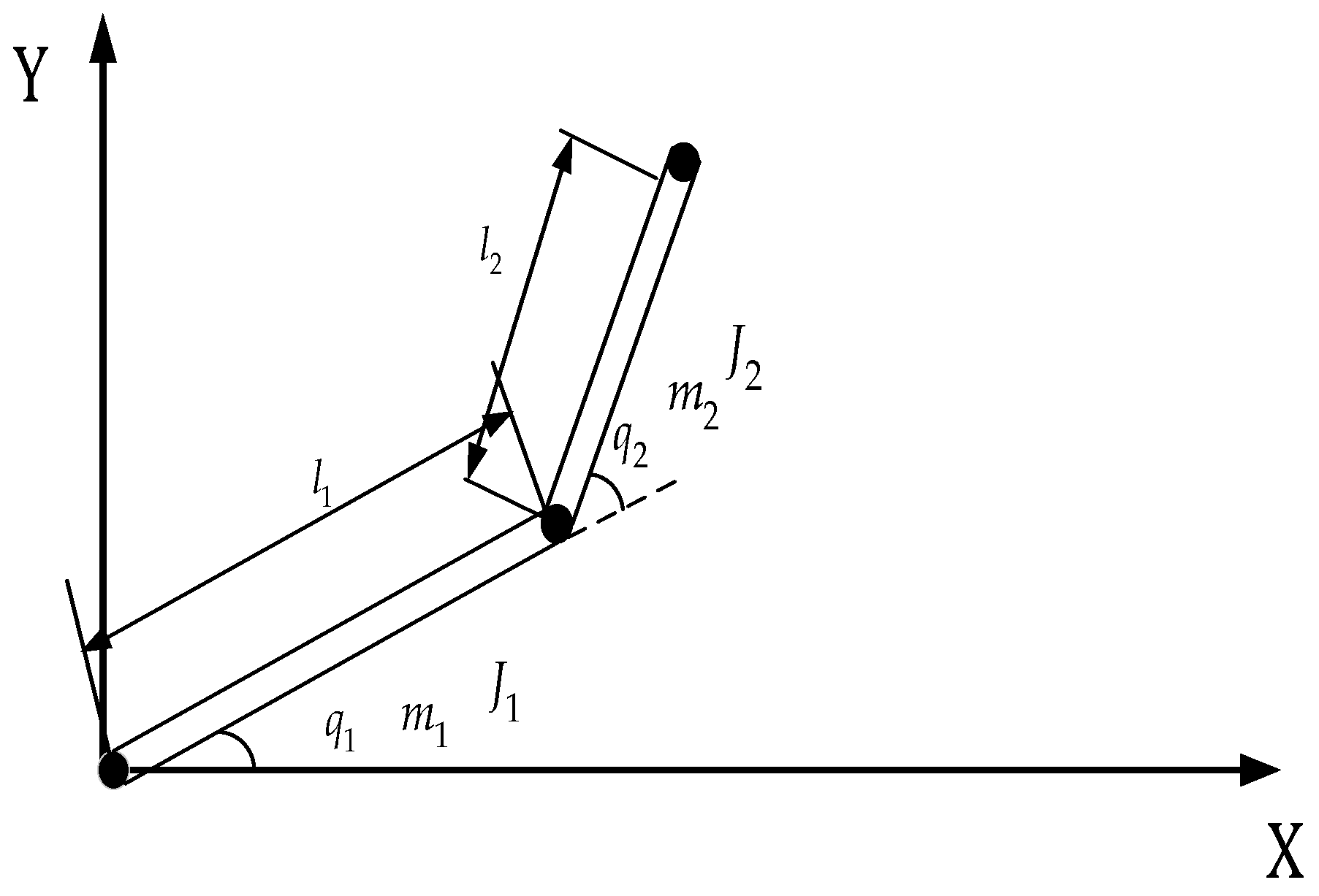
4. Application in Uncertain Robot Manipulators
5. Simulation and Experiments
5.1. Model Parameters
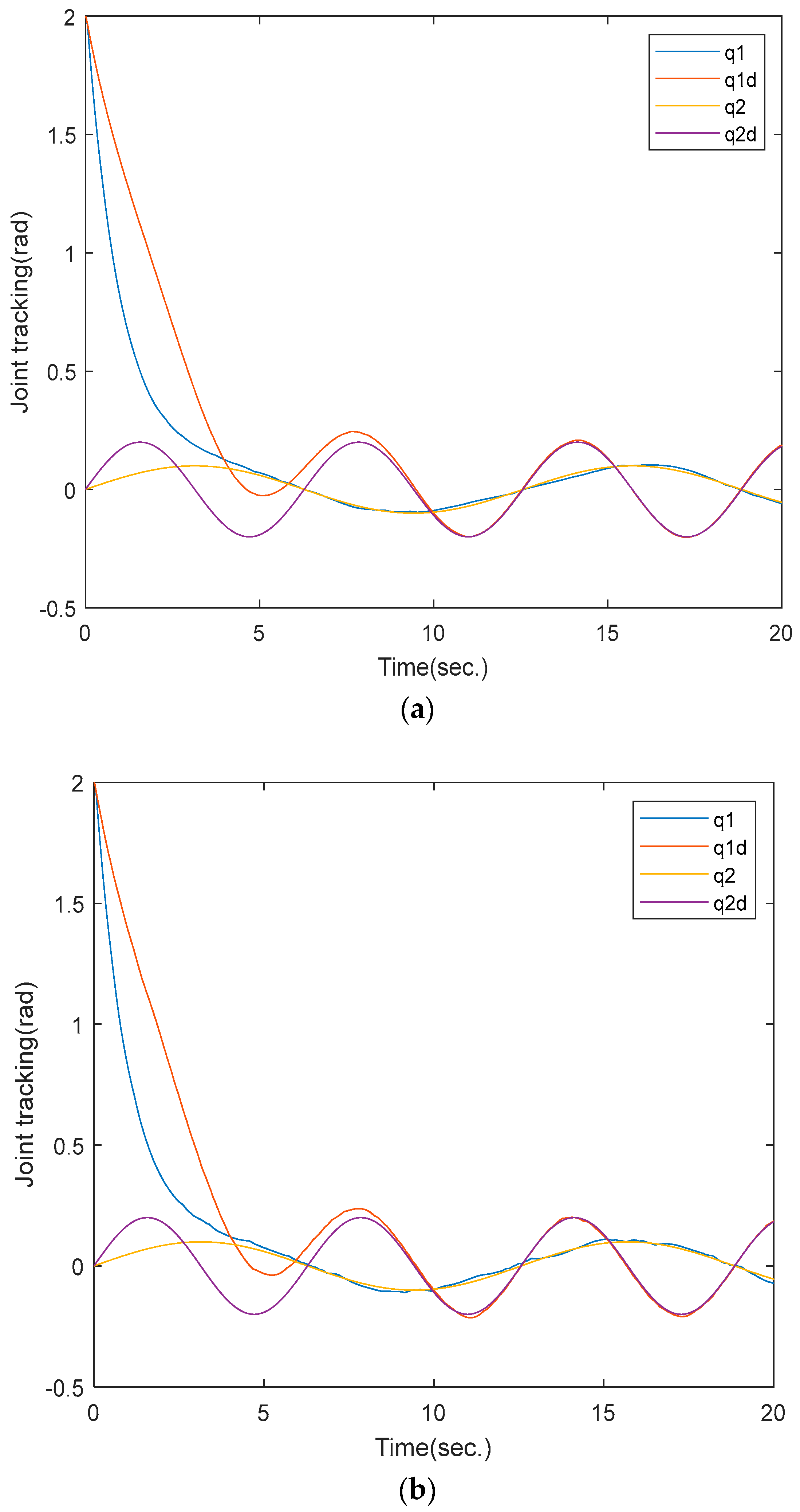
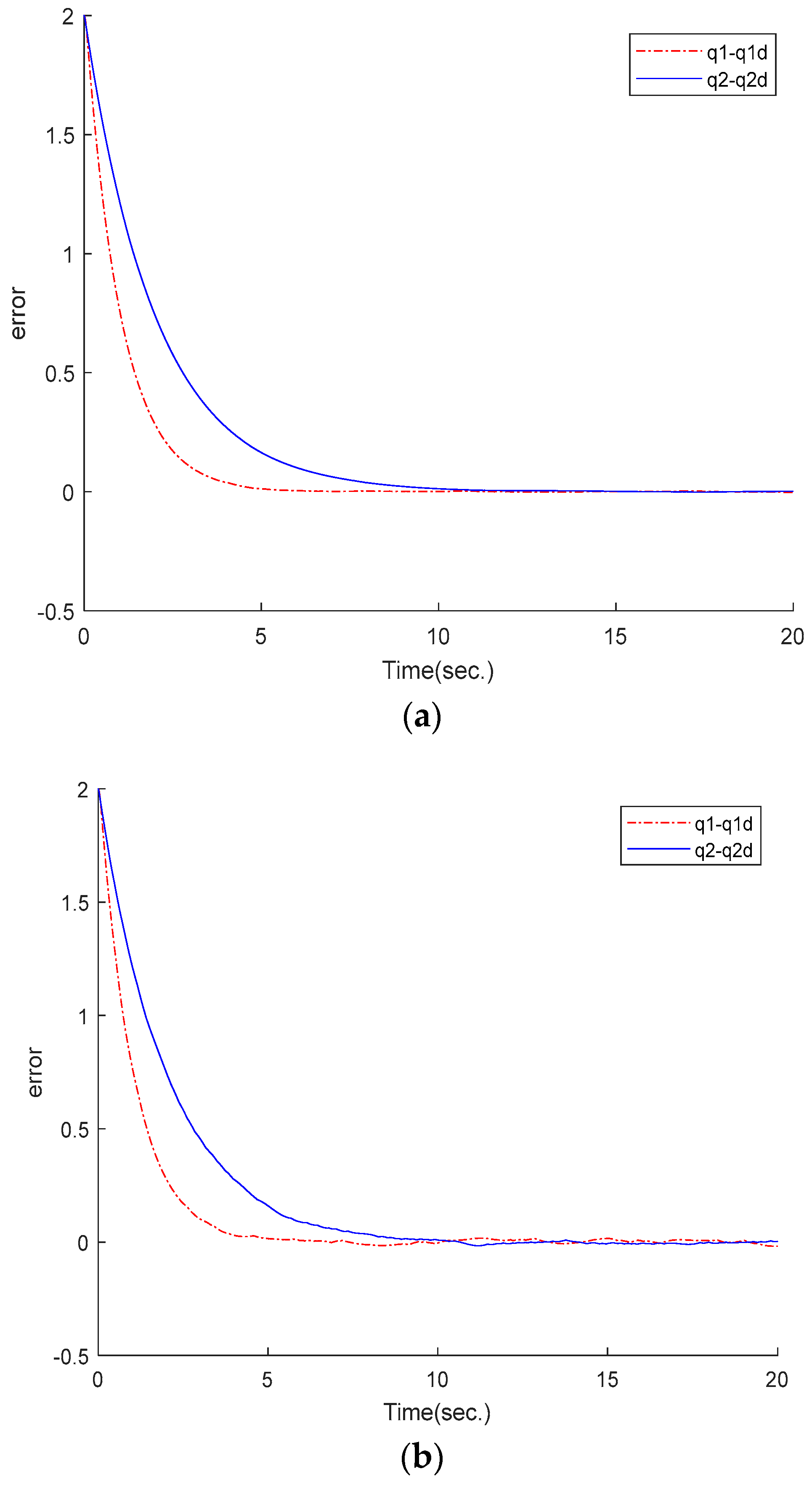
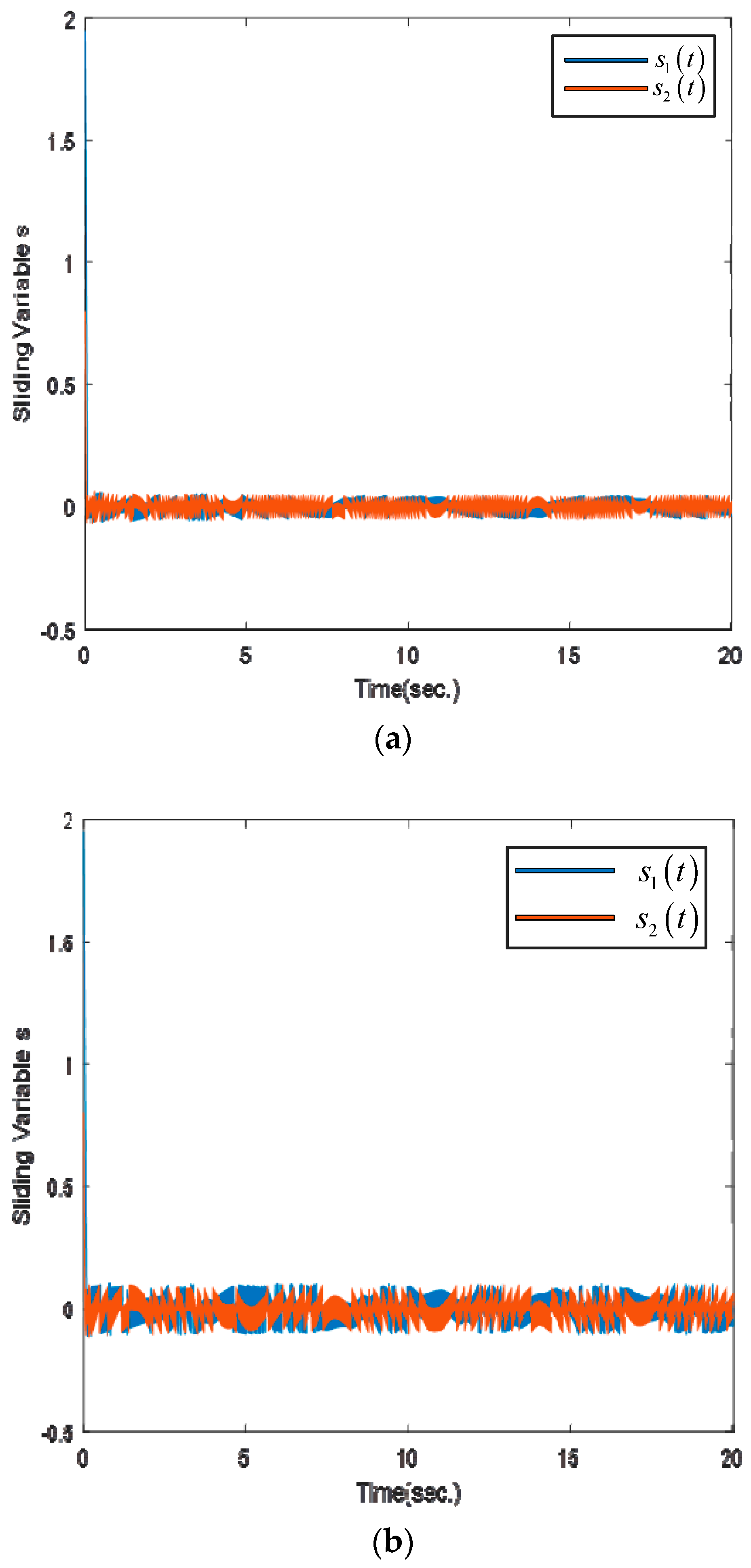
5.2. Simulation and Discussion
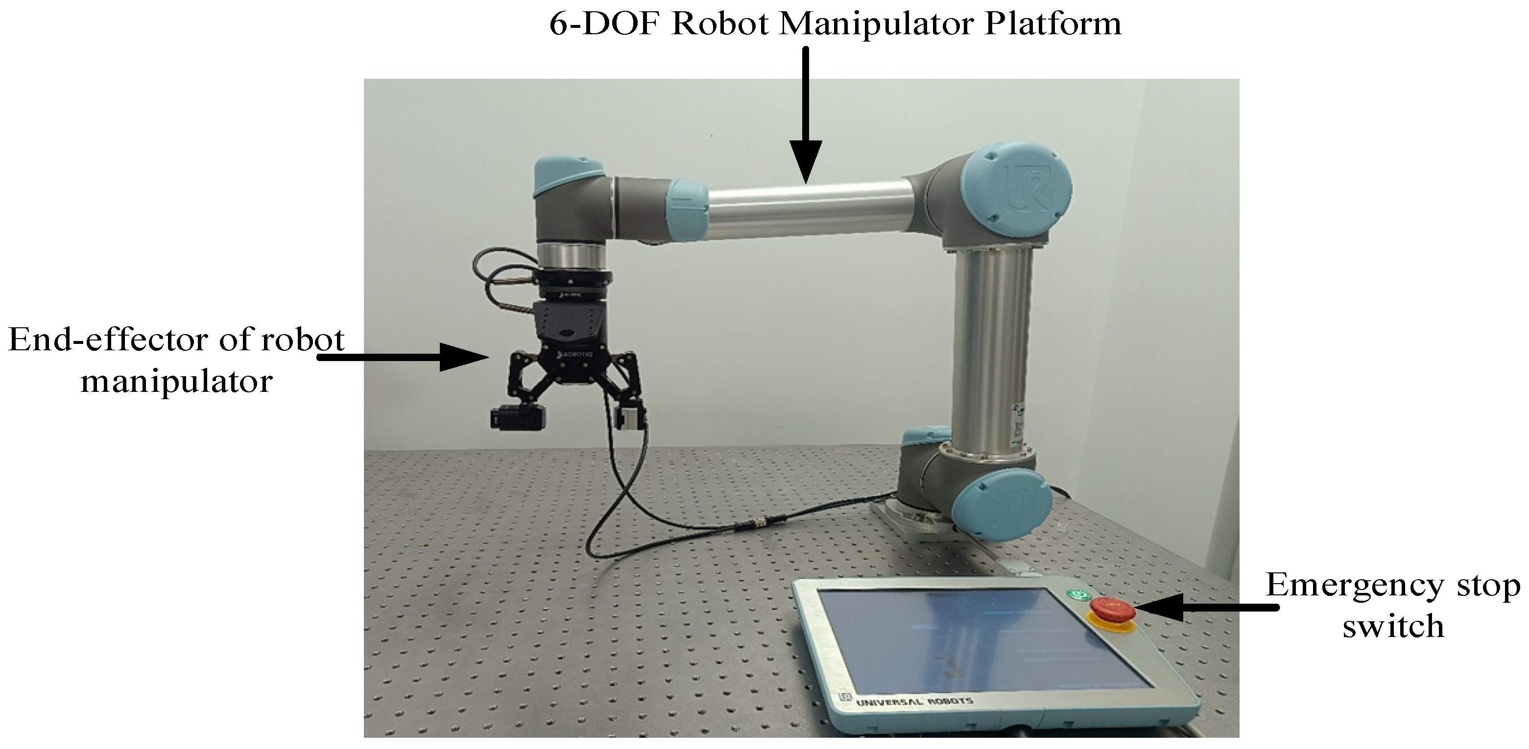
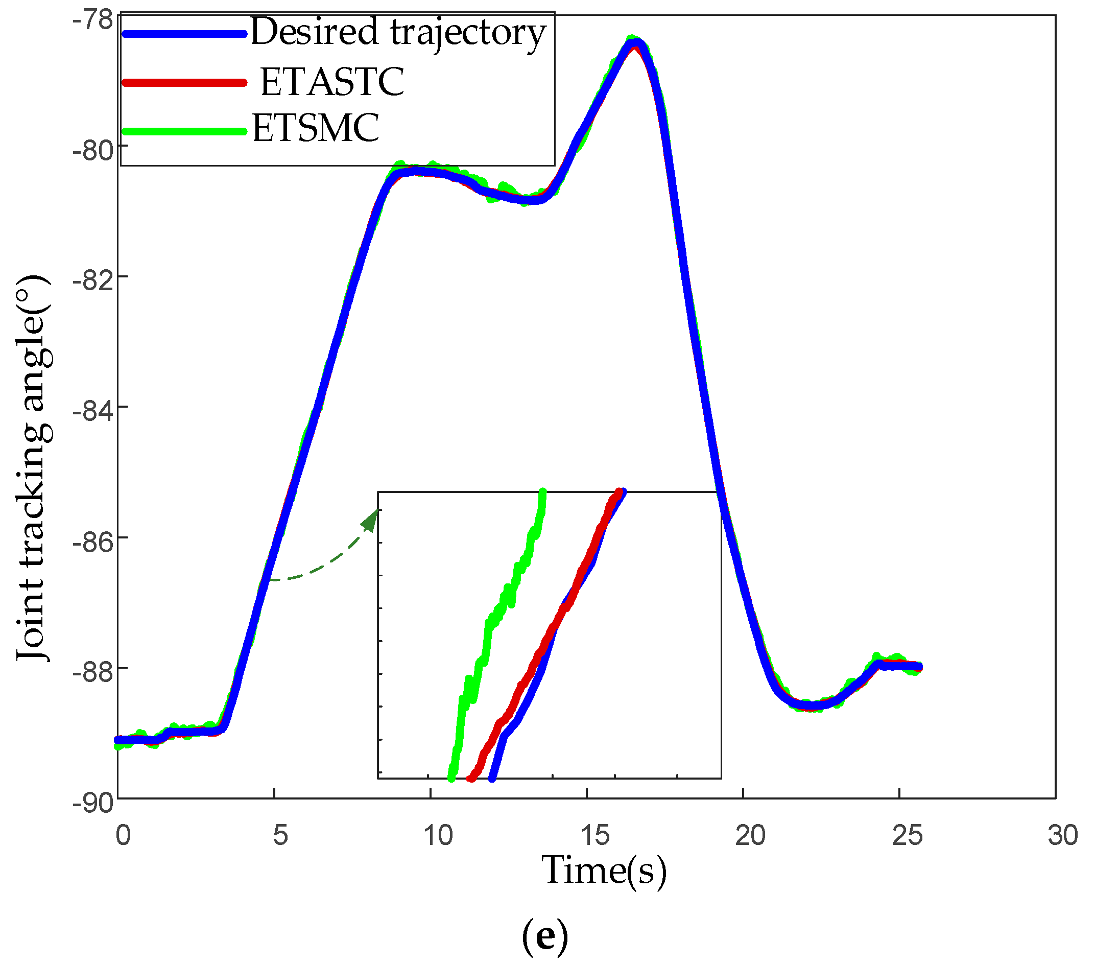
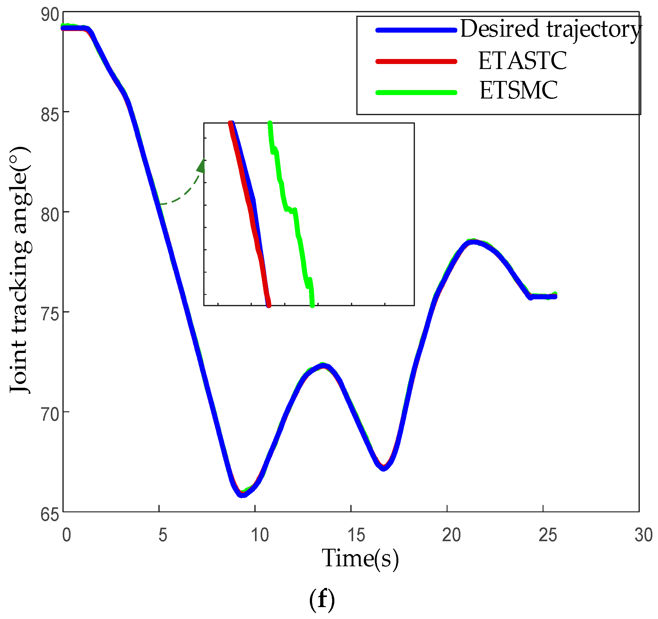
5.3. Experimental Results
6. Conclusions
Author Contributions
Funding
Institutional Review Board Statement
Informed Consent Statement
Data Availability Statement
Conflicts of Interest
References
- Tao, L.; Hui, Z. Global finite-time adaptive control for uncalibrated robot manipulator based on visual servoing. ISA Trans. 2017, 68, 402–411. [Google Scholar]
- Ma, Y.J.; Hui, Z.; Tao, L. Robust adaptive dual layer sliding mode controller: Methodology and application of uncertain robot manipulator. Trans. Inst. Meas. Control 2021, 44, 848–860. [Google Scholar] [CrossRef]
- Guo, J.P.; Lu, R.Q.; Yao, D.Y.; Zhou, Q. Implementation of the load frequency control by two approaches: Variable gain super-twisting algorithm and super-twisting-like algorithm. Nonlinear Dyn. 2018, 93, 1073–1086. [Google Scholar] [CrossRef]
- Barth, A.; Reichhartinger, K.; Wulff, K. Certainty equivalence adaptation combined with super-twisting sliding-mode control. Int. J. Control 2016, 89, 1767–1776. [Google Scholar] [CrossRef]
- Kun, L.; Zhao, K.; Gao, R. Adaptive global prescribed performance tracking control of uncertain robotic systems with unknown control directions. Int. J. Robust Nonlinear Control 2023, 33, 5956–5974. [Google Scholar]
- Mien, V.; Mavrovouniotis, M.; Ge, S.S. An Adaptive Backstepping Nonsingular Fast Terminal Sliding Mode Control for Robust Fault Tolerant Control of Robot Manipulators. IEEE Trans. Syst. Man Cybern. Syst. 2019, 49, 1448–1458. [Google Scholar]
- Liu, X.; Yang, C.; Chen, Z.; Wang, M.; Su, C.Y. Neuro-adaptive observer-based control of flexible joint robot. Neurocomputing 2018, 275, 73–82. [Google Scholar] [CrossRef]
- Zhai, J.Y.; Song, Z.B. Adaptive sliding mode trajectory tracking control for wheeled mobile robots. Int. J. Control 2019, 92, 2255–2262. [Google Scholar] [CrossRef]
- Gao, Y.; Wei, W.; Wang, X.M.; Wang, D.L. Trajectory tracking of multi-legged robot based on model predictive and sliding mode control. Inf. Sci. 2022, 606, 489–511. [Google Scholar] [CrossRef]
- Zhang, Y.Q.; Yin, Z.G.; Li, W.; Liu, J. Adaptive Sliding-Mode-Based Speed Control in Finite Control Set Model Predictive Torque Control for Induction Motors. IEEE Trans. Power Electron. 2021, 36, 8076–8087. [Google Scholar] [CrossRef]
- Li, H.Q.; Bi, L.Z.; Yi, J.G. Sliding-Mode Nonlinear Predictive Control of Brain-Controlled Mobile Robots. IEEE Trans. Cybern. 2022, 52, 5419–5431. [Google Scholar] [CrossRef]
- Tian, X.H.; Huang, X.; Liu, H.T.; Mai, Q.Q. Adaptive Fuzzy Event-Triggered Cooperative Control for Multi-Robot Systems: A Predefined-Time Strategy. Sensors 2023, 23, 7950. [Google Scholar] [CrossRef]
- Benitez, S.E.; Villarreal, M.G. Event-Triggered Control for a Three DoF Manipulator Robot. Enfoque UTE 2018, 9, 33–44. [Google Scholar] [CrossRef]
- Kamboj, A.; Dhar, N.K.; Verma, N.K. Event-Triggered Control for Trajectory Tracking by Robotic Manipulator. Comput. Intell. Theor. Appl. Future Dir. 2018, 1, 161–170. [Google Scholar]
- Erlong, K.; Yang, L.; Hong, Q. Sliding mode-based adaptive tube model predictive control for robotic manipulators with model uncertainty and state constraints. Control Theory Technol. 2023, 21, 334–351. [Google Scholar]
- Abhisek, K.; Bijnan, B. Event based robust stabilization of linear systems. In Proceedings of the IEEE Industrial Electronics Society, Dallas, TX, USA, 29 October–1 November 2014; pp. 133–138. [Google Scholar]
- Abhisek, K.; Bijnan, B. Robust Sliding Mode Control: An Event-Triggering Approach. IEEE Trans. Circuits Syst.–II Express Express Briefs 2016, 64, 146–150. [Google Scholar]
- Abhisek, K.; Bijnan, B. Event-triggered sliding mode control for a class of nonlinear systems. Int. J. Control 2016, 89, 1916–1931. [Google Scholar]
- Tian, B.L.; Cui, J.; Lu, H.; Zong, Q. Reentry Attitude Control for RLV Based on Adaptive Event-Triggered Sliding Mode. IEEE Access 2019, 7, 68429–68435. [Google Scholar] [CrossRef]
- Tian, B.L.; Cui, J.; Liu, L.; Zong, Q. Attitude Control of UAVs Based on Event-Triggered super-twisting Algorithm. IEEE Trans. Ind. Inform. 2021, 17, 1029–1038. [Google Scholar] [CrossRef]
- Bin, G.; Yong, C.; Anjian, Z. Event trigger-based adaptive sliding mode fault-tolerant control for dynamic systems. Sci. China Inf. Sci. 2021, 64, 169205:1–169205:3. [Google Scholar]
- Gian, P.I.; Antonella, F. Adaptive model-based event-triggered sliding mode control. Int. J. Adapt. Control Signal Process. 2016, 30, 1298–1316. [Google Scholar]
- Li, H.Y.; Ziran, C.; Ligang, W.; Lam, H.K.; Du, H.P. Event-Triggered Fault Detection of Nonlinear Networked Systems. IEEE Trans. Cybern. 2017, 47, 1041–1052. [Google Scholar] [CrossRef] [PubMed]
- Kiran, K.; Abhisek, K.; Bijnan, B. Event-triggered sliding mode-based tracking control for uncertain Euler-Lagrange systems. IET Control Theory Appl. 2017, 12, 1228–1235. [Google Scholar]
- Xing, L.; Wen, C.; Liu, Z.; Su, H.; Cai, J. Event-Triggered Adaptive Control for a Class of Uncertain Nonlinear Systems. IEEE Trans. Autom. Control 2017, 62, 2071–2076. [Google Scholar] [CrossRef]
- Michele, C.; Gian, P.I.; Antonella, F. Event-triggered variable structure control. Int. J. Control 2020, 93, 252–260. [Google Scholar]
- Zhiyu, L.; Siyuan, W.; Bailing, T.; Helong, L. Event-triggered-based adaptive super-twisting attitude tracking for RLV in reentry phase. J. Frankl. Inst. 2020, 357, 13430–13448. [Google Scholar]
- Pengfei, C.; Yahui, G.; Xianzhong, D. Finite-Time Disturbance Observer for Robotic Manipulator. Sensors 2019, 19, 1943. [Google Scholar] [CrossRef]
- Lei, Y.Q.; Du, F.X.; Song, H.J.; Zhang, L.P. Design and kinematics analysis of a cable-stayed notch manipulator for transluminal endoscopic surgery. Biomim. Intell. Robot. 2024, 4, 100191. [Google Scholar] [CrossRef]
- Zhang, Q.; Xu, H.; Zhu, L.; Liu, L. Positioning system design of closed-loop magnetically driven laser steering manipulator for endoscopic microsurgery. Biomim. Intell. Robot. 2023, 3, 100129. [Google Scholar] [CrossRef]


| Symbol | Definition | Value |
|---|---|---|
| Nominal mass of link 1 | 0.4 kg | |
| Nominal mass of link 2 | 1.2 kg | |
| Length of link 1 | 1.0 m | |
| Length of link 2 | 0.85 m | |
| Inertia tensor of link 1 | 2 kg·m2 | |
| Inertia tensor of link 2 | 2 kg·m2 | |
| Gravity acceleration | 9.8 m/s2 |
| Implementation Technique | Number of Control Updating Instants | ) |
|---|---|---|
| Event triggering () | 530 | |
| Periodic control () | 1075 | |
| Periodic control () | 830 |
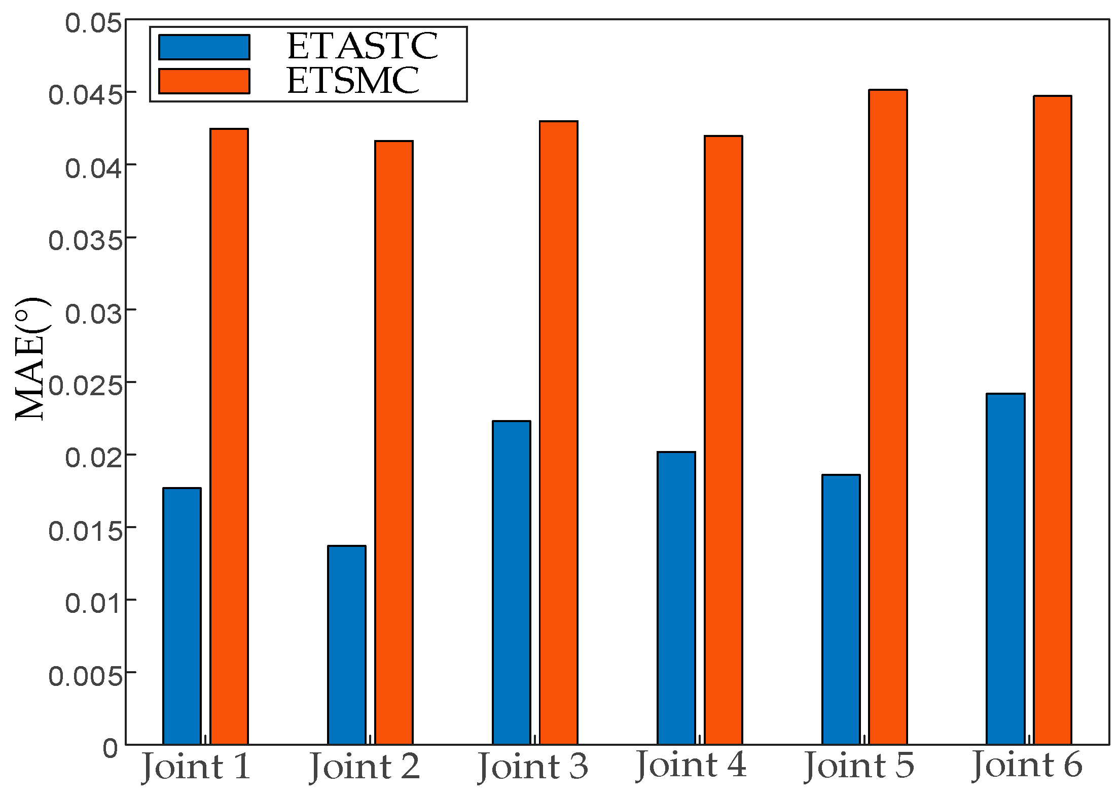
| Degrees of Freedom | ETASTC | ETSMC |
|---|---|---|
| Joint 1 | 0.0176 | 0.0424 |
| Joint 2 | 0.0137 | 0.0416 |
| Joint 3 | 0.0223 | 0.0429 |
| Joint 4 | 0.0201 | 0.0419 |
| Joint 5 | 0.0186 | 0.0451 |
| Joint 6 | 0.0242 | 0.0447 |
| Mean | 0.0194 | 0.0430 |
Disclaimer/Publisher’s Note: The statements, opinions and data contained in all publications are solely those of the individual author(s) and contributor(s) and not of MDPI and/or the editor(s). MDPI and/or the editor(s) disclaim responsibility for any injury to people or property resulting from any ideas, methods, instructions or products referred to in the content. |
© 2025 by the authors. Licensee MDPI, Basel, Switzerland. This article is an open access article distributed under the terms and conditions of the Creative Commons Attribution (CC BY) license (https://creativecommons.org/licenses/by/4.0/).
Share and Cite
Ma, Y.; Zhao, H.; Li, T. Adaptive Super-Twisting Tracking for Uncertain Robot Manipulators Based on the Event-Triggered Algorithm. Sensors 2025, 25, 1616. https://doi.org/10.3390/s25051616
Ma Y, Zhao H, Li T. Adaptive Super-Twisting Tracking for Uncertain Robot Manipulators Based on the Event-Triggered Algorithm. Sensors. 2025; 25(5):1616. https://doi.org/10.3390/s25051616
Chicago/Turabian StyleMa, Yajun, Hui Zhao, and Tao Li. 2025. "Adaptive Super-Twisting Tracking for Uncertain Robot Manipulators Based on the Event-Triggered Algorithm" Sensors 25, no. 5: 1616. https://doi.org/10.3390/s25051616
APA StyleMa, Y., Zhao, H., & Li, T. (2025). Adaptive Super-Twisting Tracking for Uncertain Robot Manipulators Based on the Event-Triggered Algorithm. Sensors, 25(5), 1616. https://doi.org/10.3390/s25051616