
Multijoint Continuous Motion Estimation for Human Lower Limb Based on Surface Electromyography


Abstract
1. Introduction
2. Experimental Setup
2.1. Experimental Design
- Gait: Each participant completed this experiment in approximately 5.5 s, with a walking speed controlled at 2 m/s, performing a total of 5 trials. Gait involves the dynamic changes of lower limb joints during walking, which helps analyze the joint angle variations and gait cycle of normal walking. Although this speed (equivalent to 7.2 km/h) exceeds typical walking speeds (usually around 1.2–1.5 m/s), it was deliberately chosen to simulate brisk walking or rapid movement conditions, offering a more thorough evaluation of the model’s performance in such scenarios.
- Obstacle Crossing: Each participant completed this experiment in approximately 5 s, performing a total of 5 trials. Obstacle crossing simulates lower limb movements when stepping over an obstacle, providing angle change data for rapid movements within a short time.
- Squatting: Each participant completed this experiment in approximately 25 s, with 10 repetitions of each squatting action, performing a total of 5 trials. This movement pattern is designed to simulate the squatting and standing actions in daily life and is suitable for studying dynamic control and joint angle variations in the lower limbs.
- Knee Flexion–Extension: Each participant completed this experiment in approximately 20 s, with 10 repetitions of each knee flexion–extension action, performing a total of 5 trials. This movement pattern primarily focuses on the flexion–extension of the knee joint and effectively tests the continuous variation in the knee joint angle.
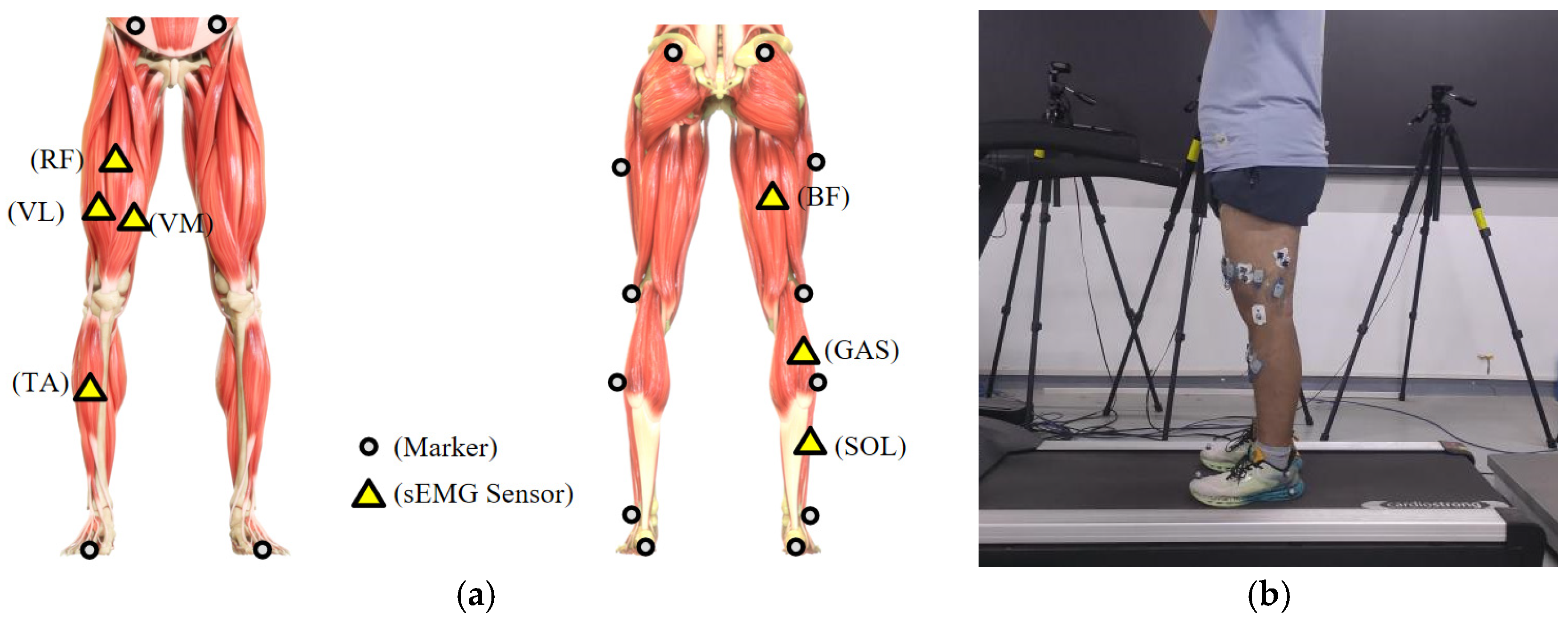
2.2. Data Collection
2.3. Data Processing
2.4. Sliding Window Data Expansion Strategy
3. Methods
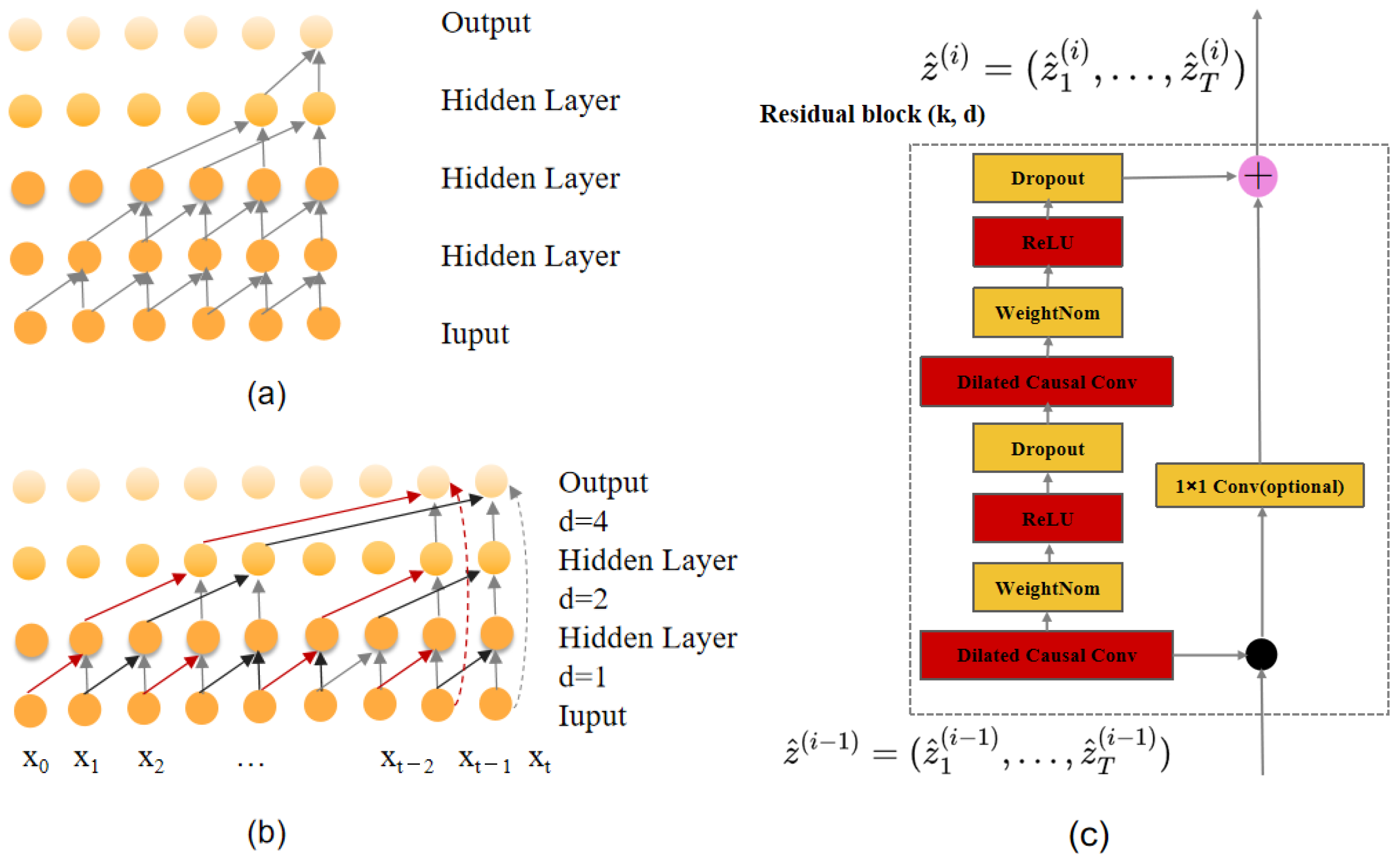
3.1. TCN
3.1.1. Causal Convolution
3.1.2. Dilated Convolution
3.1.3. Residual Module
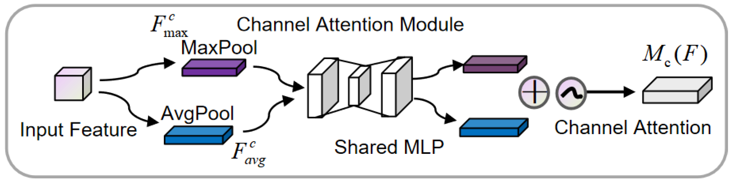
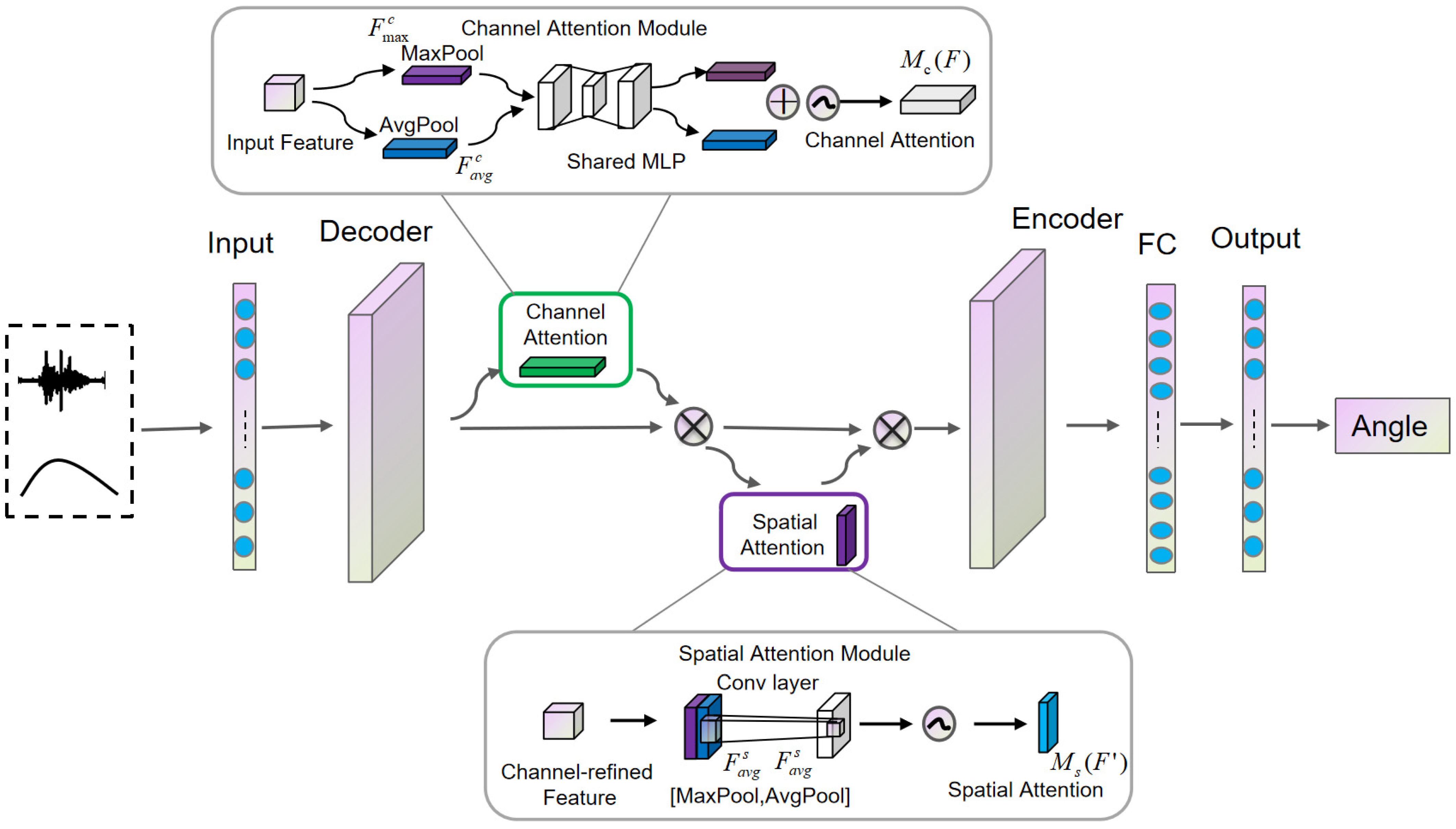
3.2. CBAM
3.3. CB-TCN
3.4. Evaluation Metrics
3.5. Model Comparison
- (1)
- ED-TCN
- (2)
- TCN
- (3)
- LSTM
- (4)
- Wiener Filter
4. Results
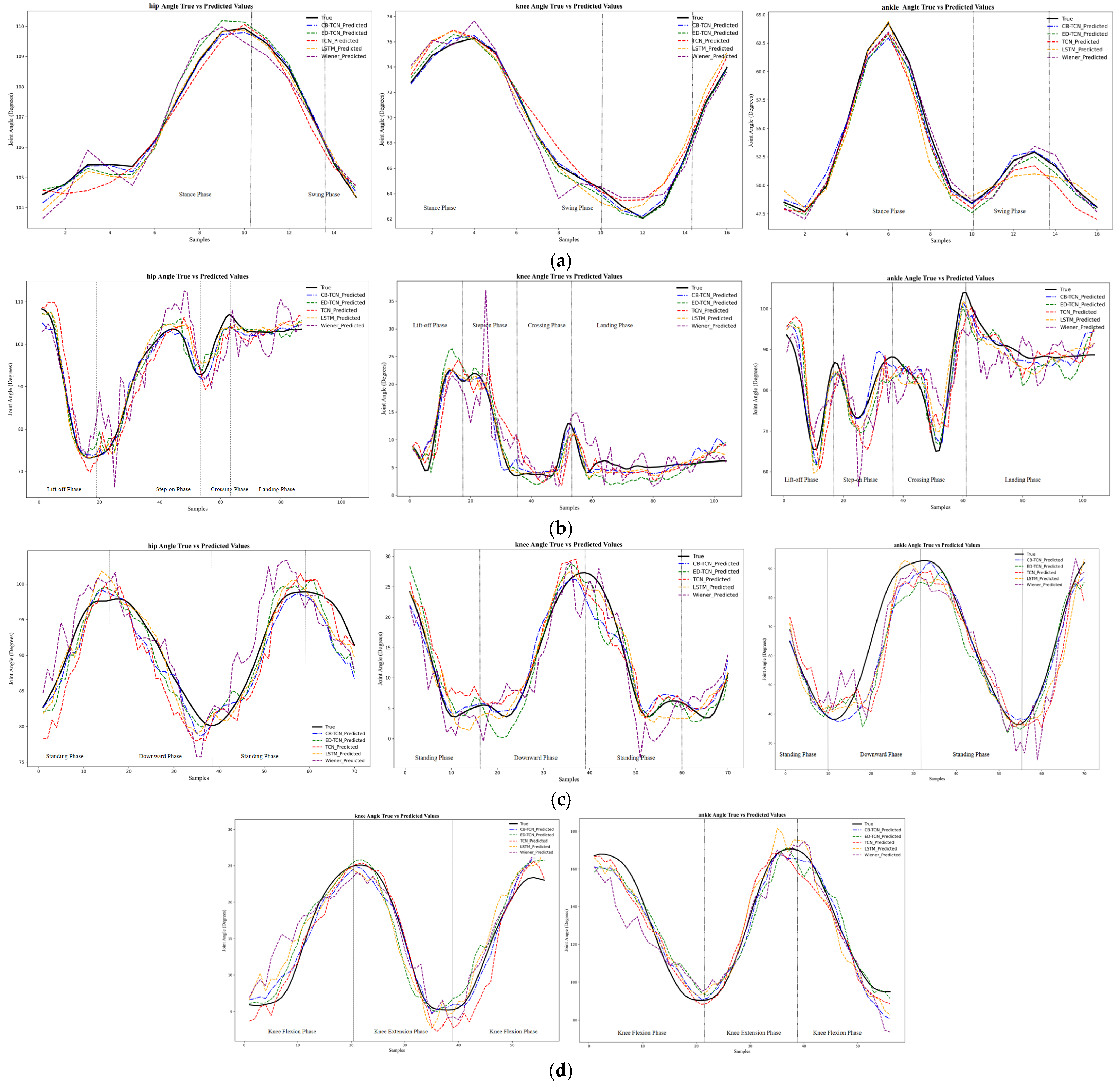
4.1. Angle Estimation Curve Analysis
- (1)
- Gait Motion
- (2)
- Obstacle Crossing Motion
- (3)
- Squat and Stand Motion
- (4)
- Knee Flexion–Extension Motion
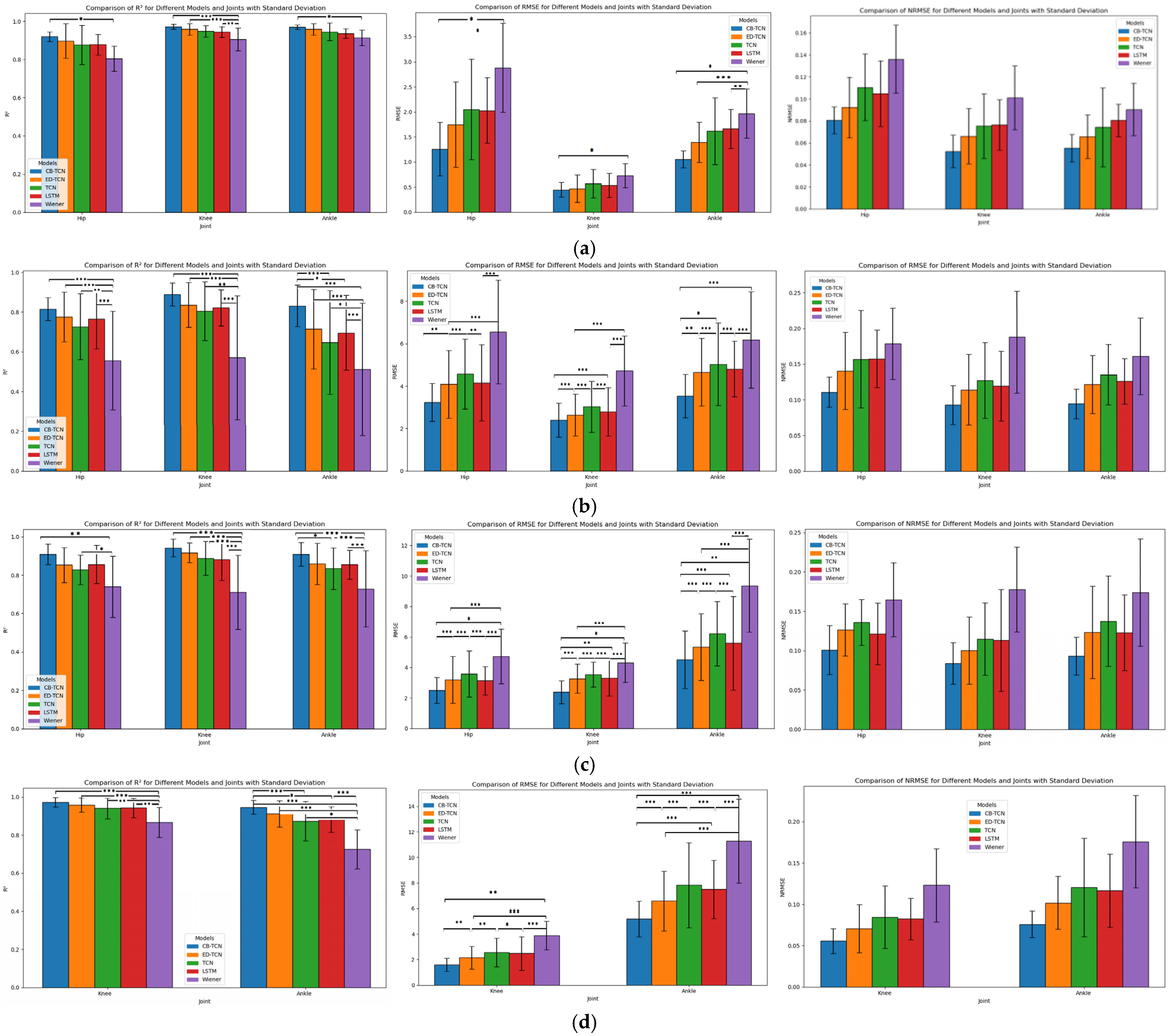
4.2. Comparison Analysis of the CB-TCN Model with Other Models
- (1)
- Gait Motion
- (2)
- Obstacle Crossing Motion
- (3)
- Squat and Stand Motion
- (4)
- Flexion–Extension Motion
4.3. Real-Time Analysis
5. Conclusions
Supplementary Materials
Author Contributions
Funding
Institutional Review Board Statement
Informed Consent Statement
Data Availability Statement
Acknowledgments
Conflicts of Interest
References
- Sarajchi, M.; Al-Hares, M.K.; Sirlantzis, K. Wearable lower-limb exoskeleton for children with cerebral palsy: A systematic review of mechanical design, actuation type, control strategy, and clinical evaluation. IEEE Trans. Neural Syst. Rehabil. Eng. 2021, 29, 2695–2720. [Google Scholar] [CrossRef] [PubMed]
- Wang, G.; Jin, L.; Zhang, J.; Duan, X.; Yi, J.; Zhang, M.; Sun, Z. Recurrent Neural Network Enabled Continuous Motion Estimation of Lower Limb Joints from Incomplete sEMG Signals. IEEE Trans. Neural Syst. Rehabil. Eng. 2024, 32, 3577–3589. [Google Scholar] [CrossRef] [PubMed]
- Zhou, J.; Yang, S.; Xue, Q. Lower limb rehabilitation exoskeleton robot: A review. Adv. Mech. Eng. 2021, 13, 16878140211011862. [Google Scholar] [CrossRef]
- Li, W.Z.; Cao, G.Z.; Zhu, A.B. Review on control strategies for lower limb rehabilitation exoskeletons. IEEE Access 2021, 9, 123040–123060. [Google Scholar] [CrossRef]
- Gordleeva, S.Y.; Lobov, S.A.; Grigorev, N.A.; Savosenkov, A.O.; Shamshin, M.O.; Lukoyanov, M.V.; Khoruzhko, M.A.; Kazantsev, V.B. Real-time EEG–EMG human–machine interface-based control system for a lower-limb exoskeleton. IEEE Access 2020, 8, 84070–84081. [Google Scholar] [CrossRef]
- Chen, D.; Cai, Y.; Qian, X.; Ansari, R.; Xu, W.; Chu, K.-C.; Huang, M.-C. Bring gait lab to everyday life: Gait analysis in terms of activities of daily living. IEEE Internet Things J. 2019, 7, 1298–1312. [Google Scholar] [CrossRef]
- Scherpereel, K.; Molinaro, D.; Inan, O.; Shepherd, M.; Young, A. A human lower-limb biomechanics and wearable sensors dataset during cyclic and non-cyclic activities. Sci. Data 2023, 10, 924. [Google Scholar] [CrossRef]
- Kuang, Y.; Wu, Q.; Shao, J.; Wu, J.; Wu, X. Extreme learning machine classification method for lower limb movement recognition. Clust. Comput. 2017, 20, 3051–3059. [Google Scholar] [CrossRef]
- Qin, P.; Shi, X. Evaluation of feature extraction and classification for lower limb motion based on sEMG signal. Entropy 2020, 22, 852. [Google Scholar] [CrossRef]
- Wu, X.; Yuan, Y.; Zhang, X.; Wang, C.; Xu, T.; Tao, D. Gait phase classification for a lower limb exoskeleton system based on a graph convolutional network model. IEEE Trans. Ind. Electron. 2021, 69, 4999–5008. [Google Scholar] [CrossRef]
- Sun, Z.; Zhang, X.; Liu, K.; Shi, T.; Wang, J. A multi-joint continuous motion estimation method of lower limb using least squares support vector machine and zeroing neural network based on semg signals. Neural Process. Lett. 2023, 55, 2867–2884. [Google Scholar] [CrossRef]
- Wang, F.; Lu, J.; Fan, Z.; Ren, C.; Geng, X. Continuous motion estimation of lower limbs based on deep belief networks and random forest. Rev. Sci. Instrum. 2022, 93, 044106. [Google Scholar] [CrossRef] [PubMed]
- Li, W.; Liu, K.; Sun, Z.; Li, C.; Chai, Y.; Gu, J. A neural network-based model for lower limb continuous estimation against the disturbance of uncertainty. Biomed. Signal Process. Control 2022, 71, 103115. [Google Scholar] [CrossRef]
- Sommer, L.F. EMG-Driven Exoskeleton Control; Universidade de São Paulo: São Paulo, Brazil, 2019. [Google Scholar]
- Xie, H.; Li, G.; Zhao, X.; Li, F. Prediction of limb joint angles based on multi-source signals by GS-GRNN for exoskeleton wearer. Sensors 2020, 20, 1104. [Google Scholar] [CrossRef] [PubMed]
- Liu, G.; Zhang, L.; Han, B.; Zhang, T.; Wang, Z.; Wei, P. sEMG-based continuous estimation of knee joint angle using deep learning with convolutional neural network. In Proceedings of the 2019 IEEE 15th international conference on automation science and engineering (CASE), Vancouver, BC, Canada, 22–26 August 2019; pp. 140–145. [Google Scholar]
- Song, Q.; Ma, X.; Liu, Y. Continuous online prediction of lower limb joints angles based on sEMG signals by deep learning approach. Comput. Biol. Med. 2023, 163, 107124. [Google Scholar] [CrossRef] [PubMed]
- Ma, C.; Guo, W.; Zhang, H.; Samuel, O.W.; Ji, X.; Xu, L.; Li, G. A novel and efficient feature extraction method for deep learning based continuous estimation. IEEE Robot. Autom. Lett. 2021, 6, 7341–7348. [Google Scholar] [CrossRef]
- Ding, G.; Plummer, A.; Georgilas, I. Deep learning with an attention mechanism for continuous biomechanical motion estimation across varied activities. Front. Bioeng. Biotechnol. 2022, 10, 1021505. [Google Scholar] [CrossRef]
- Fan, J.; Zhang, K.; Huang, Y.; Zhu, Y.; Chen, B. Parallel spatio-temporal attention-based TCN for multivariate time series prediction. Neural Comput. Appl. 2023, 35, 13109–13118. [Google Scholar] [CrossRef]
- Chen, C.; Guo, W.; Ma, C.; Yang, Y.; Wang, Z.; Lin, C. sEMG-based continuous estimation of finger kinematics via large-scale temporal convolutional network. Appl. Sci. 2021, 11, 4678. [Google Scholar] [CrossRef]
- Wang, F.; Liang, W.; Afzal, H.M.R.; Fan, A.; Li, W.; Dai, X.; Liu, S.; Hu, Y.; Li, Z.; Yang, P. Estimation of Lower Limb Joint Angles and Joint Moments during Different Locomotive Activities Using the Inertial Measurement Units and a Hybrid Deep Learning Model. Sensors 2023, 23, 9039. [Google Scholar] [CrossRef]
- Du, J.; Liu, Z.; Dong, W.; Zhang, W.; Miao, Z. A Novel TCN-LSTM Hybrid Model for sEMG-Based Continuous Estimation of Wrist Joint Angles. Sensors 2024, 24, 5631. [Google Scholar] [CrossRef] [PubMed]
- Hamner, S.R.; Delp, S.L. Muscle contributions to fore-aft and vertical body mass center accelerations over a range of running speeds. J. Biomech. 2013, 46, 780–787. [Google Scholar] [CrossRef]
- Hermens, H.; Frenks, H.B. Surface electromyography application areas and parameters. In Proceedings of the Third General SENIAM Workshop, Aachen, Germany, 15–16 May 1998. [Google Scholar]
- Liang, J.; Shi, Z.; Zhu, F.; Chen, W.; Chen, X.; Li, Y. Gaussian process autoregression for joint angle prediction based on sEMG signals. Front. Public Health 2021, 9, 685596. [Google Scholar] [CrossRef]
- Wahid, M.F.; Tafreshi, R.; Langari, R. A multi-window majority voting strategy to improve hand gesture recognition accuracies using electromyography signal. IEEE Trans. Neural Syst. Rehabil. Eng. 2019, 28, 427–436. [Google Scholar] [CrossRef]
- Ma, C.; Li, W.; Cao, J.; Du, J.; Li, Q.; Gravina, R. Adaptive sliding window based activity recognition for assisted livings. Inf. Fusion 2020, 53, 55–65. [Google Scholar] [CrossRef]
- Hewage, P.; Behera, A.; Trovati, M.; Pereira, E.; Ghahremani, M.; Palmieri, F.; Liu, Y. Temporal convolutional neural (TCN) network for an effective weather forecasting using time-series data from the local weather station. Soft Comput. 2020, 24, 16453–16482. [Google Scholar] [CrossRef]
- Tsinganos, P.; Jansen, B.; Cornelis, J.; Skodras, A. Real-time analysis of hand gesture recognition with temporal convolutional networks. Sensors 2022, 22, 1694. [Google Scholar] [CrossRef]
- Wang, S.; Huang, L.; Jiang, D.; Sun, Y.; Jiang, G.; Li, J.; Zou, C.; Fan, H.; Xie, Y.; Xiong, H.; et al. Improved multi-stream convolutional block attention module for sEMG-based gesture recognition. Front. Bioeng. Biotechnol. 2022, 10, 909023. [Google Scholar] [CrossRef]
- Zanghieri, M.; Benatti, S.; Burrello, A.; Kartsch, V.; Conti, F.; Benini, L. Robust real-time embedded EMG recognition framework using temporal convolutional networks on a multicore IoT processor. IEEE Trans. Biomed. Circuits Syst. 2019, 14, 244–256. [Google Scholar] [CrossRef]
- Kirti; Rajpal, N. A multi-crop disease identification approach based on residual attention learning. J. Intell. Syst. 2023, 32, 20220248. [Google Scholar] [CrossRef]


| Activity | Hip Joint (ms) | Knee Joint (ms) | Ankle Joint (ms) |
| Walking | 13.20 ± 0.048 | 13.53 ± 0.124 | 13.46 ± 0.056 |
| Obstacle Crossing | 34.59 ± 0.068 | 34.31 ± 0.044 | 34.01 ± 0.072 |
| Squatting | 28.68 ± 0.064 | 28.68 ± 0.076 | 27.77 ± 0.060 |
| Knee Flexion-Extension | 27.17 ± 0.060 | 27.18 ± 0.048 | 27.18 ± 0.048 |
Disclaimer/Publisher’s Note: The statements, opinions and data contained in all publications are solely those of the individual author(s) and contributor(s) and not of MDPI and/or the editor(s). MDPI and/or the editor(s) disclaim responsibility for any injury to people or property resulting from any ideas, methods, instructions or products referred to in the content. |
© 2025 by the authors. Licensee MDPI, Basel, Switzerland. This article is an open access article distributed under the terms and conditions of the Creative Commons Attribution (CC BY) license (https://creativecommons.org/licenses/by/4.0/).
Share and Cite
Han, Y.; Tao, Q.; Zhang, X. Multijoint Continuous Motion Estimation for Human Lower Limb Based on Surface Electromyography. Sensors 2025, 25, 719. https://doi.org/10.3390/s25030719
Han Y, Tao Q, Zhang X. Multijoint Continuous Motion Estimation for Human Lower Limb Based on Surface Electromyography. Sensors. 2025; 25(3):719. https://doi.org/10.3390/s25030719
Chicago/Turabian StyleHan, Yonglin, Qing Tao, and Xiaodong Zhang. 2025. "Multijoint Continuous Motion Estimation for Human Lower Limb Based on Surface Electromyography" Sensors 25, no. 3: 719. https://doi.org/10.3390/s25030719
APA StyleHan, Y., Tao, Q., & Zhang, X. (2025). Multijoint Continuous Motion Estimation for Human Lower Limb Based on Surface Electromyography. Sensors, 25(3), 719. https://doi.org/10.3390/s25030719