
Applying MLP-Mixer and gMLP to Human Activity Recognition

Abstract
1. Introduction
- We apply and evaluate MLP-based models (MLP-Mixer and gMLP) on HAR tasks, assessing their performance in terms of accuracy and computational efficiency, measured by the number of parameters. Additionally, we apply prominent CNN models originally proposed as image classification models to HAR and compare their results.
- We investigate the effects of parameter reduction by systematically examining the impact of decreasing the number of parameters in both MLP-Mixer and gMLP models. This analysis provides insights into the optimal level of parameter reduction when adapting MLP-based models for HAR applications. Furthermore, we clarified the FLOPs and actual training time for each model. These results serve as valuable metrics when evaluating models from an efficiency perspective. Our findings potentially lead to more efficient model designs in HAR.
2. Related Works
2.1. CNN-Based Models in HAR
2.2. RNNs and Attention-Based Models in HAR
2.3. MLP-Based Models in HAR
3. Methods
3.1. Patch Embedding for Sensor Data Processing
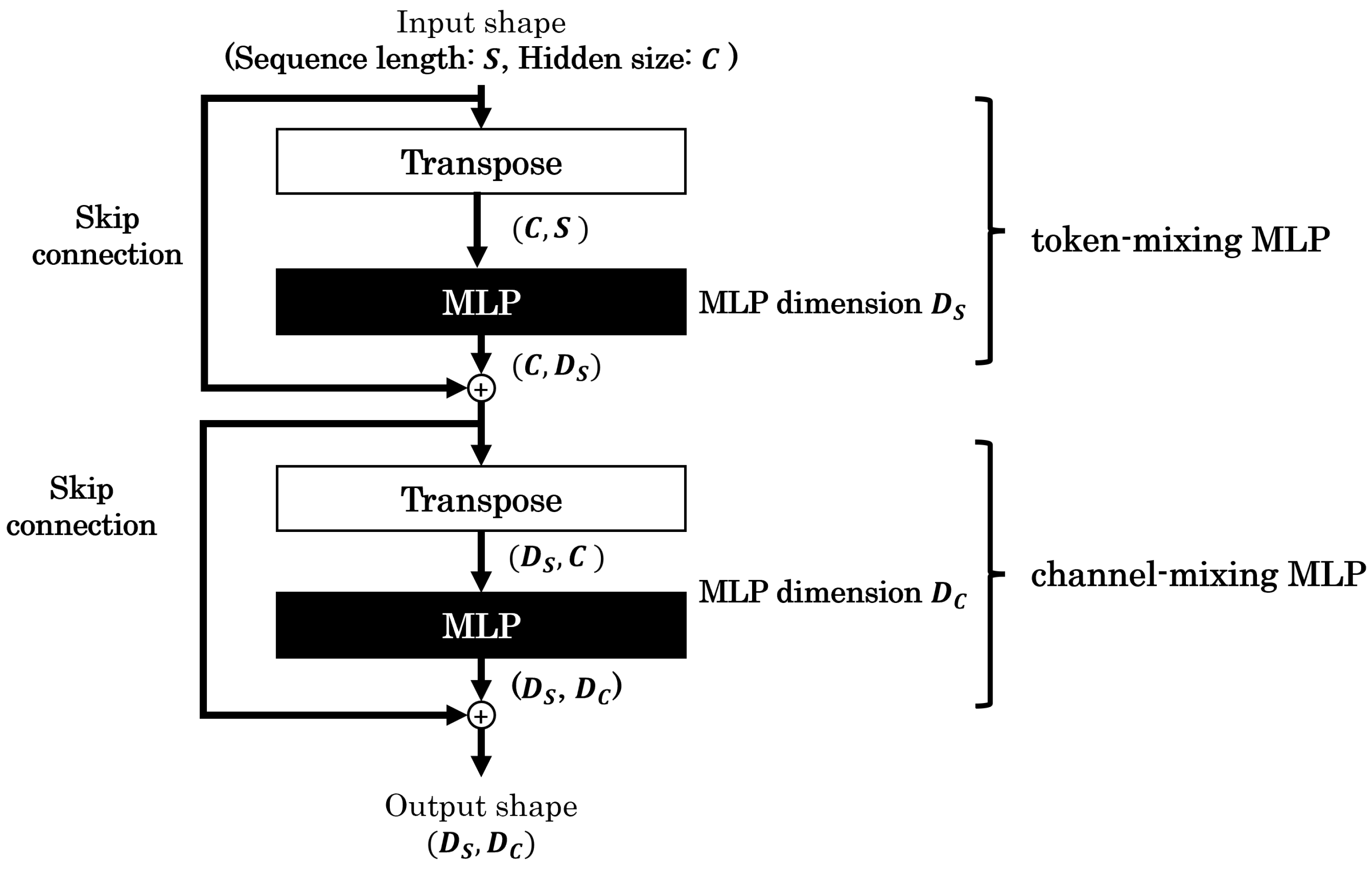
3.2. MLP-Mixer
- Patch resolution: P;
- Hidden size: C;
- The number of Mixer layers;
- The output dimension of the token-mixing MLP layer: ;
- The output dimension of the channel-mixing MLP layer: .
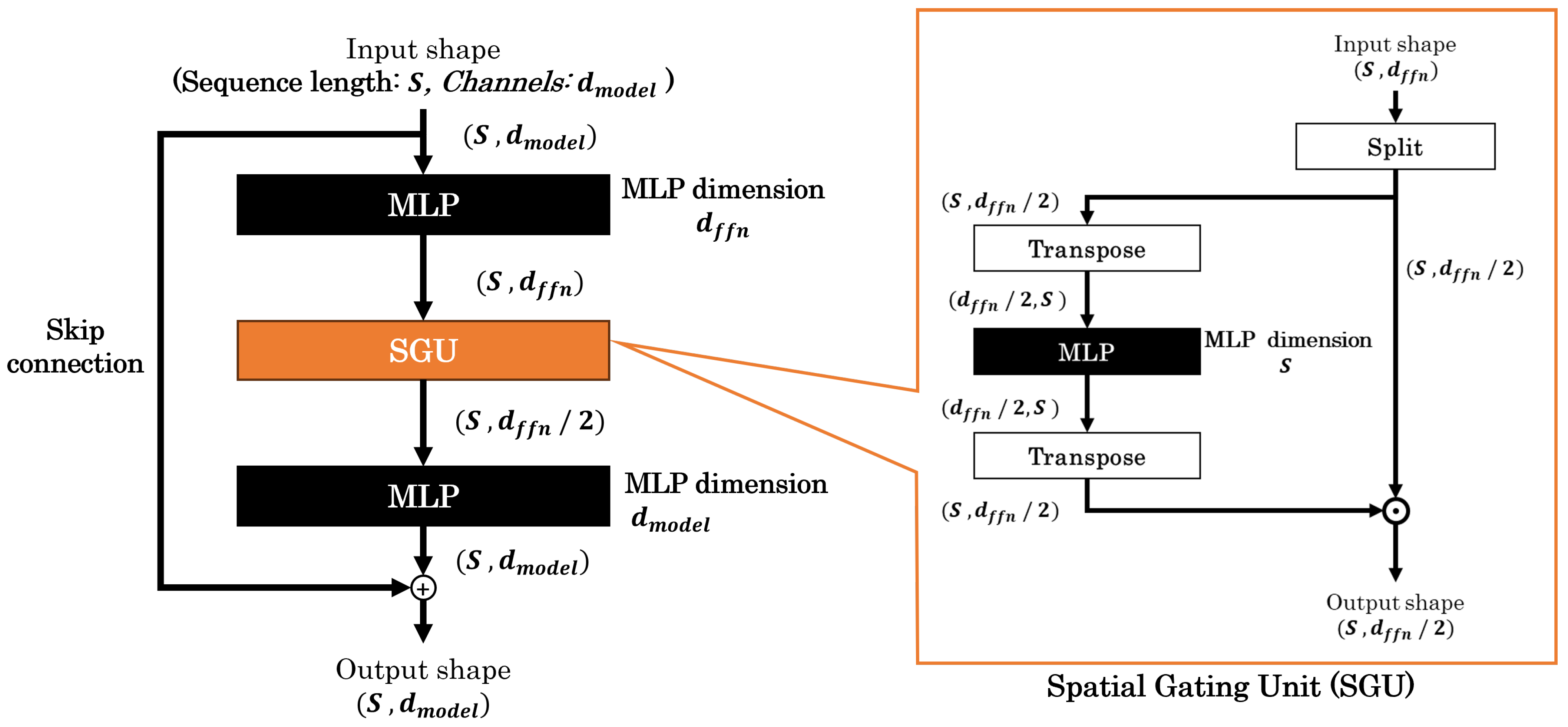
3.3. gMLP
- Patch resolution: P;
- The number of gMLP blocks;
- The first MLP output dimensions in gMLP block: ;
- -
- is also used to calculate the number of channels for the input tokens (corresponding to C in MLP-Mixer).
- The second MLP output dimensions in gMLP block: .
4. Experiments
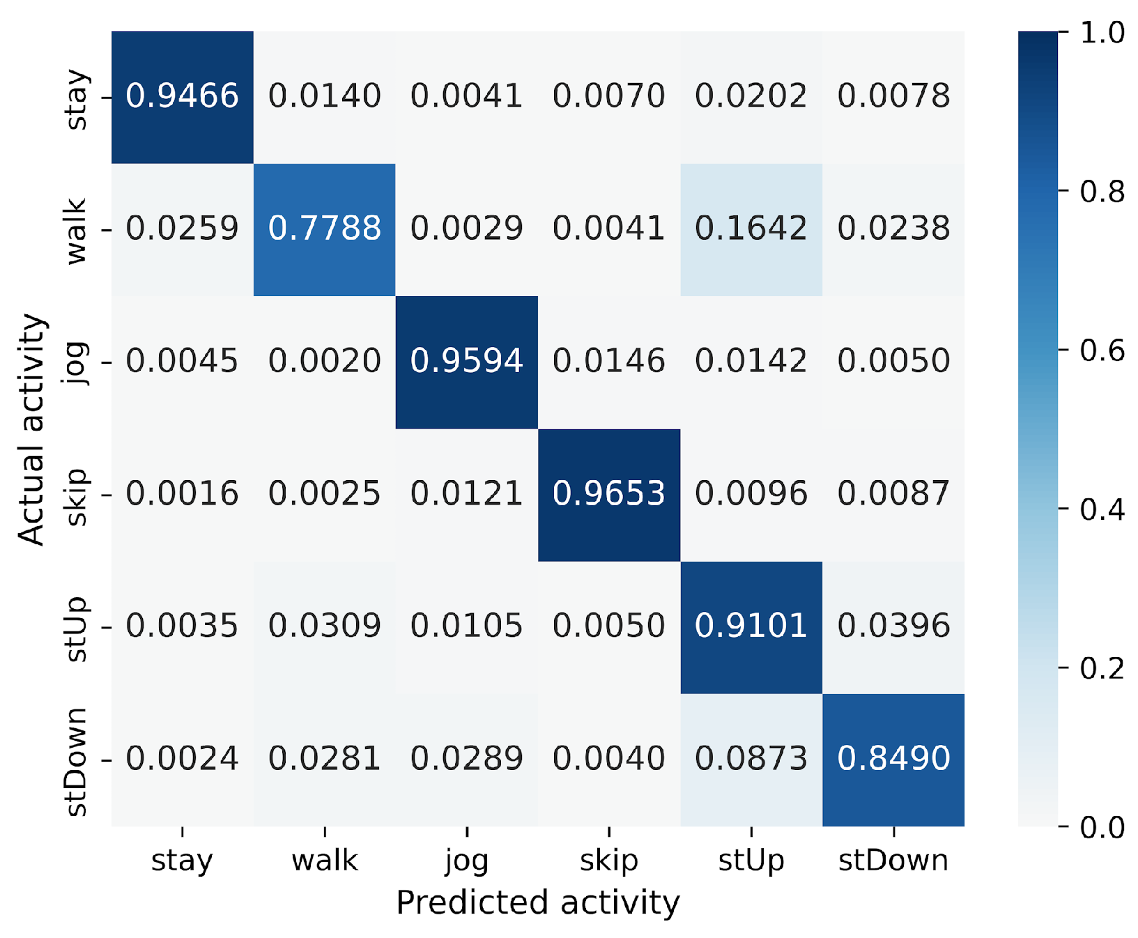
4.1. Datasets
4.2. Experimental Settings
- Hidden size: C;
- The output dimension of the token-mixing MLP layer: ;
- The output dimension of the channel-mixing MLP layer: .
- The first MLP output dimensions in gMLP block and the number of channels for the input tokens: ;
- The second MLP output dimensions in gMLP block: .
- Batch size: 256;
- Optimizer function: Adam;
- Learning rate: 0.0001;
- Epochs: 100.
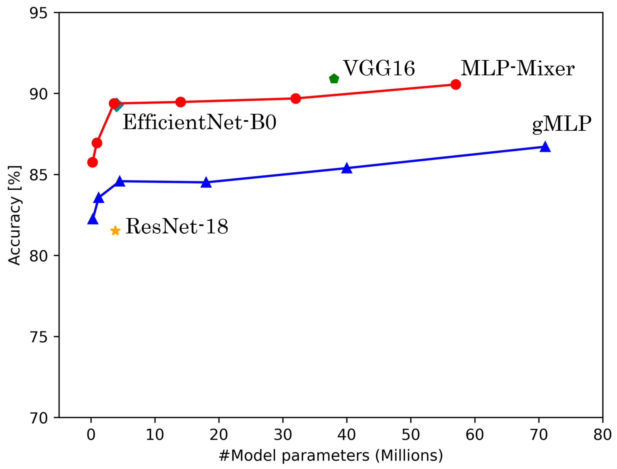
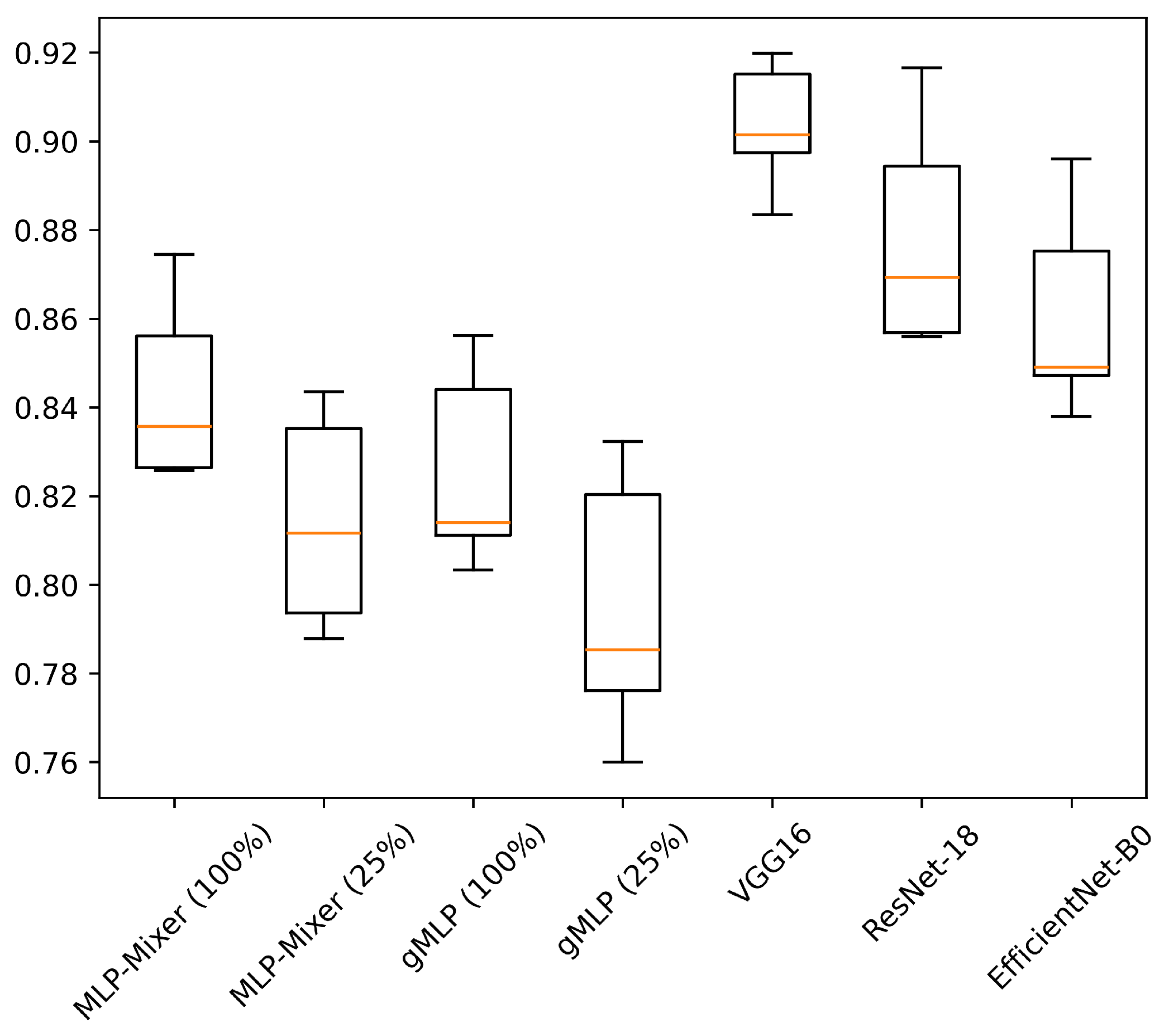
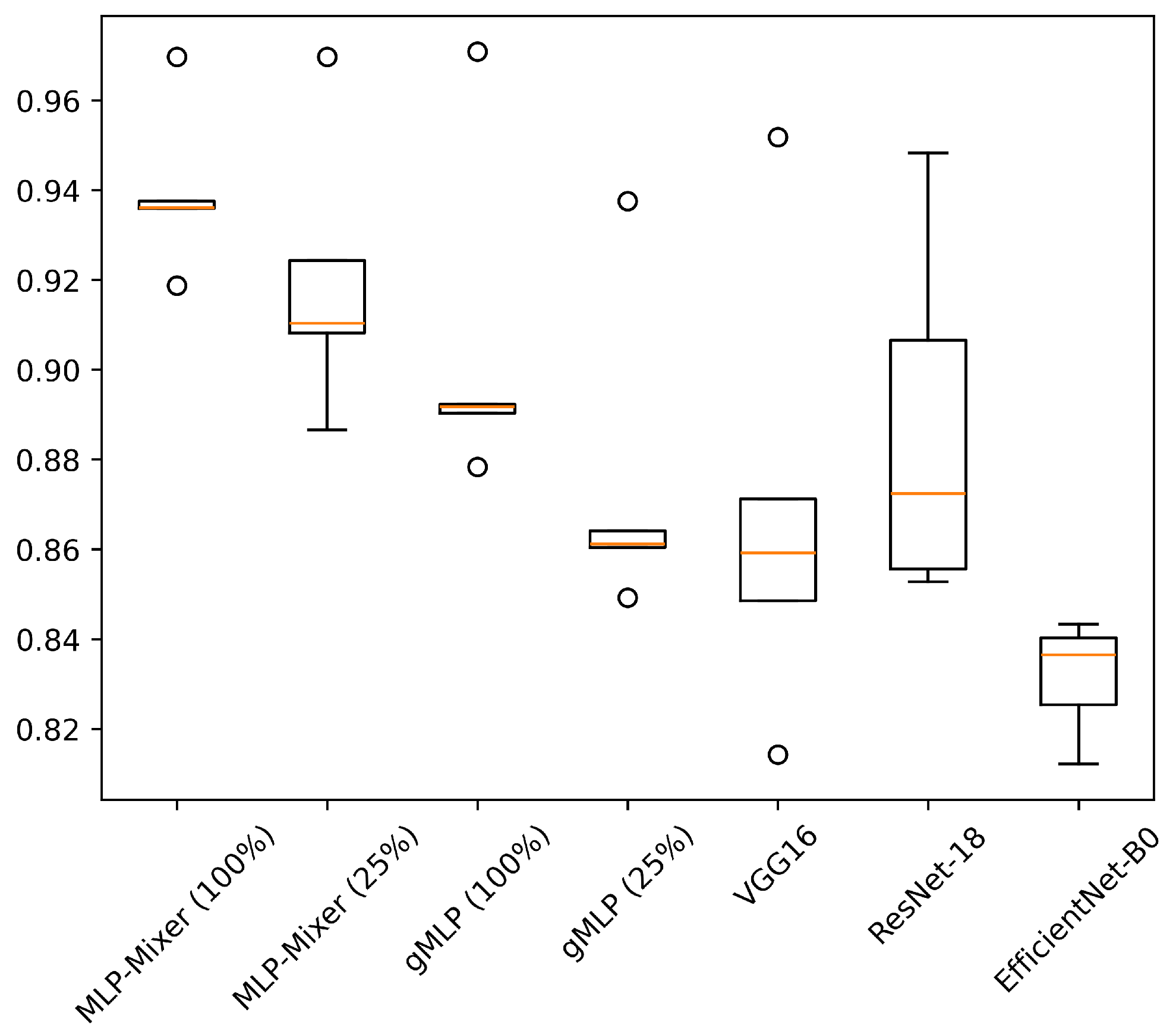
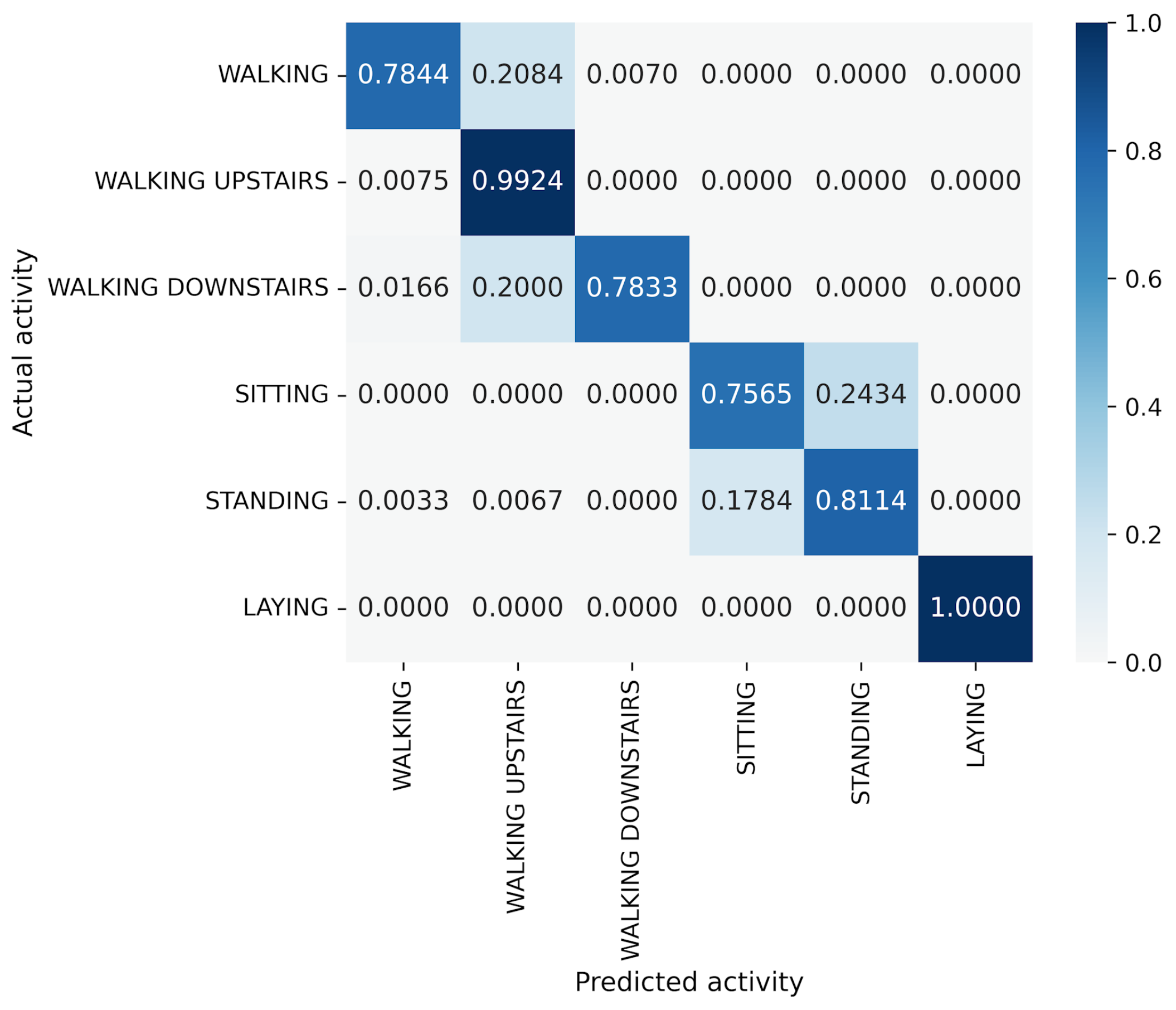
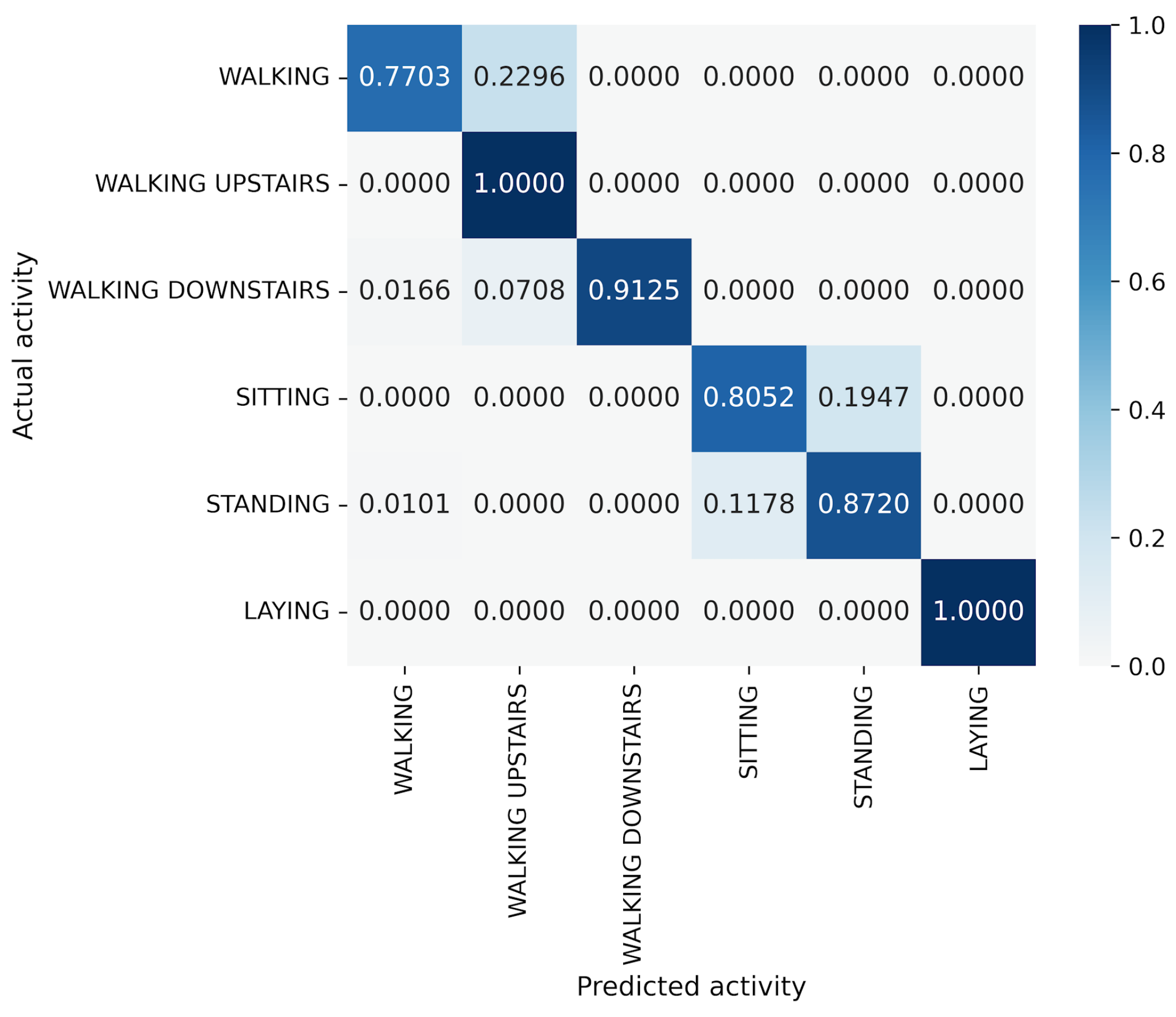
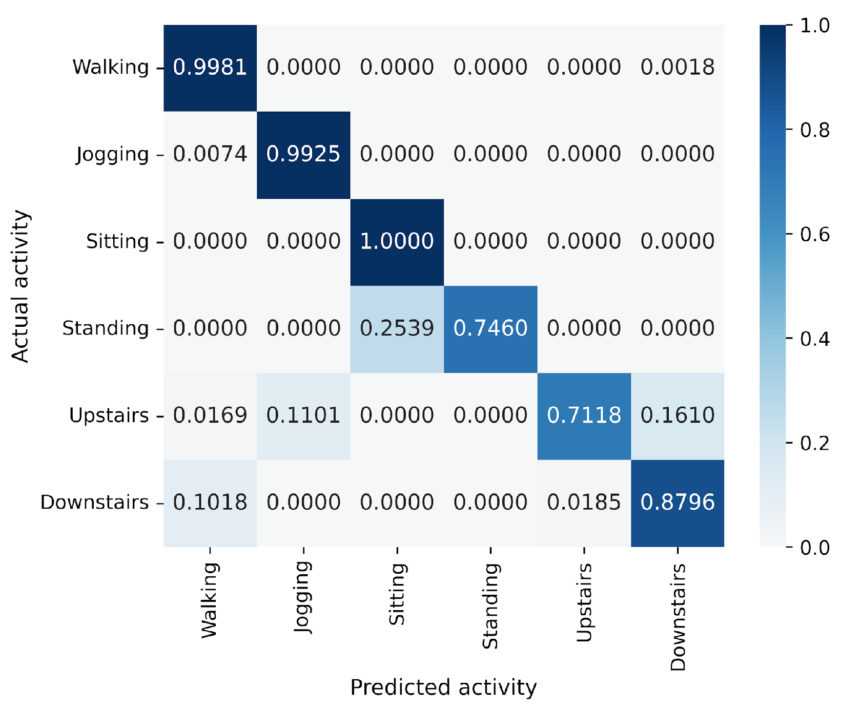
5. Results
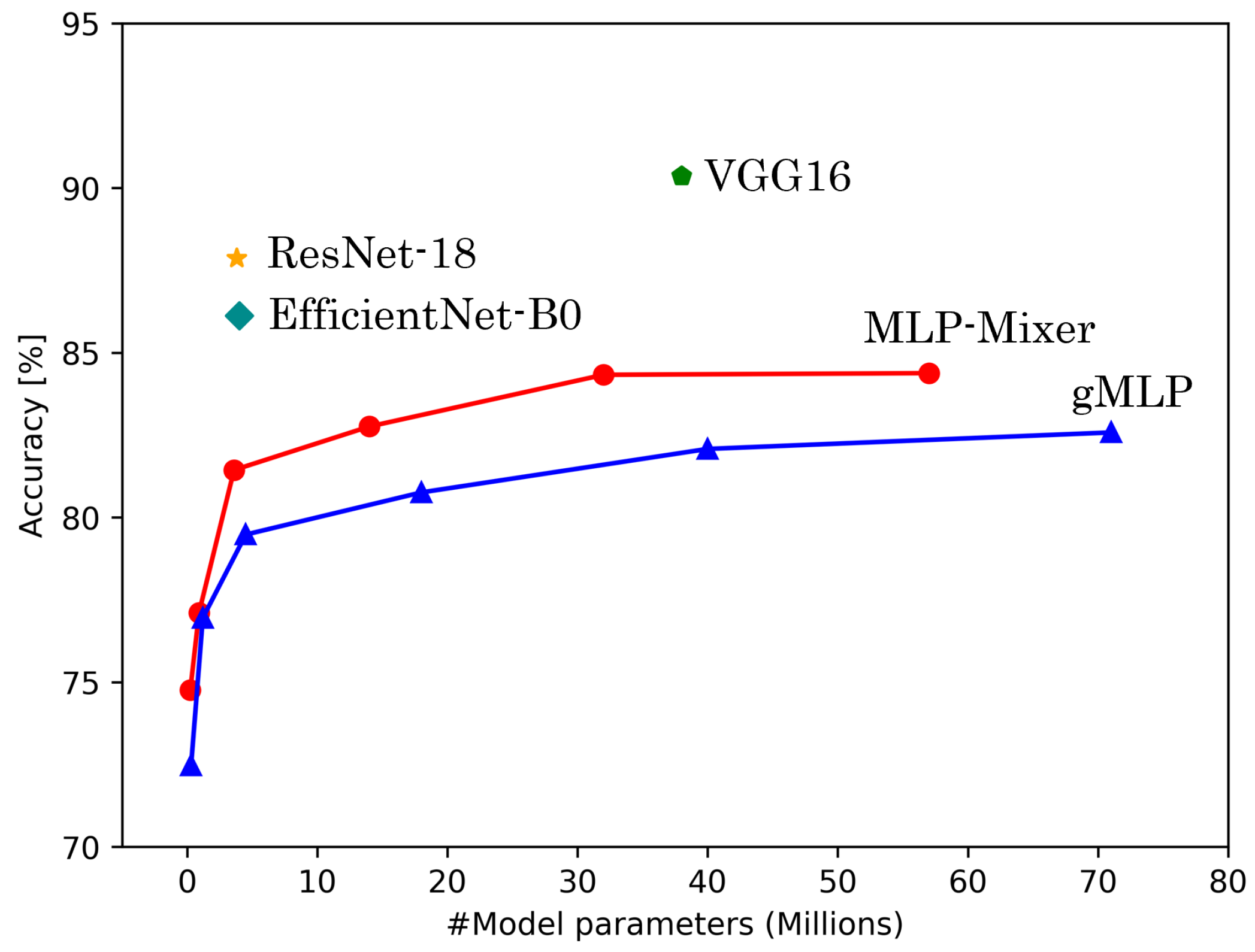
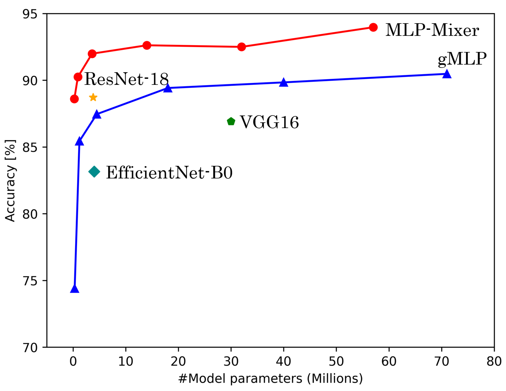
5.1. Accuracy and Model Parameters
5.2. Training Time and Latency
5.3. Limitations
6. Conclusions
Author Contributions
Funding
Institutional Review Board Statement
Informed Consent Statement
Data Availability Statement
Conflicts of Interest
References
- Attal, F.; Mohammed, S.; Dedabrishvili, M.; Chamroukhi, F.; Oukhellou, L.; Amirat, Y. Physical Human Activity Recognition Using Wearable Sensors. Sensors 2015, 15, 31314–31338. [Google Scholar] [CrossRef]
- De, D.; Bharti, P.; Das, S.K.; Chellappan, S. Multimodal Wearable Sensing for Fine-Grained Activity Recognition in Healthcare. IEEE Internet Comput. 2015, 19, 26–35. [Google Scholar] [CrossRef]
- Apple. Available online: https://support.apple.com/ja-jp/guide/iphone/ipha5dddb411/ios (accessed on 26 November 2024).
- Dosovitskiy, A.; Beyer, L.; Kolesnikov, A.; Weissenborn, D.; Zhai, X.; Unterthiner, T.; Dehghani, M.; Minderer, M.; Heigold, G.; Gelly, S.; et al. An Image is Worth 16x16 Words: Transformers for Image Recognition at Scale. In Proceedings of the International Conference on Learning Representations, Virtual, 3–7 May 2021. [Google Scholar]
- Tolstikhin, I.O.; Houlsby, N.; Kolesnikov, A.; Beyer, L.; Zhai, X.; Unterthiner, T.; Yung, J.; Steiner, A.; Keysers, D.; Uszkoreit, J.; et al. MLP-Mixer: An all-MLP Architecture for Vision. In Proceedings of the Advances in Neural Information Processing Systems, Virtual, 6–14 December 2021; Curran Associates, Inc.: Red Hook, NY, USA, 2021; Volume 34, pp. 24261–24272. [Google Scholar]
- Liu, H.; Dai, Z.; So, D.; Le, Q.V. Pay Attention to MLPs. In Proceedings of the Advances in Neural Information Processing Systems, Virtual, 6–14 December 2021; Ranzato, M., Beygelzimer, A., Dauphin, Y., Liang, P., Vaughan, J.W., Eds.; Curran Associates, Inc.: Red Hook, NY, USA, 2021; Volume 34, pp. 9204–9215. [Google Scholar]
- Tran, D.N.; Phan, D.D. Human Activities Recognition in Android Smartphone Using Support Vector Machine. In Proceedings of the 2016 7th International Conference on Intelligent Systems, Modelling and Simulation (ISMS), Bangkok, Thailand, 25–27 January 2016; pp. 64–68. [Google Scholar]
- Bayat, A.; Pomplun, M.; Tran, D.A. A Study on Human Activity Recognition Using Accelerometer Data from Smartphones. Procedia Comput. Sci. 2014, 34, 450–457. [Google Scholar] [CrossRef]
- Gao, X.; Luo, H.; Wang, Q.; Zhao, F.; Ye, L.; Zhang, Y. A Human Activity Recognition Algorithm Based on Stacking Denoising Autoencoder and LightGBM. Sensors 2019, 19, 947. [Google Scholar] [CrossRef]
- Simonyan, K.; Zisserman, A. Very Deep Convolutional Networks for Large-Scale Image Recognition. In Proceedings of the 3rd International Conference on Learning Representations, ICLR 2015, San Diego, CA, USA, 7–9 May 2015. [Google Scholar]
- He, K.; Zhang, X.; Ren, S.; Sun, J. Deep Residual Learning for Image Recognition. In Proceedings of the 2016 IEEE Conference on Computer Vision and Pattern Recognition (CVPR), Las Vegas, NV, USA, 27–30 June 2016; pp. 770–778. [Google Scholar] [CrossRef]
- Tan, M.; Le, Q. EfficientNet: Rethinking Model Scaling for Convolutional Neural Networks. In Proceedings of the 36th International Conference on Machine Learning, PMLR, Long Beach, CA, USA, 9–15 June 2019; Volume 97, pp. 6105–6114. [Google Scholar]
- Vaswani, A. Attention is all you need. Adv. Neural Inf. Process. Syst. 2017, 30, 5998–6008. [Google Scholar]
- Zeng, M.; Nguyen, L.T.; Yu, B.; Mengshoel, O.J.; Zhu, J.; Wu, P.; Zhang, J. Convolutional Neural Networks for human activity recognition using mobile sensors. In Proceedings of the 6th International Conference on Mobile Computing, Applications and Services, Austin, TX, USA, 6–7 November 2014; pp. 197–205. [Google Scholar] [CrossRef]
- Ismail, W.N.; Alsalamah, H.A.; Hassan, M.M.; Mohamed, E. AUTO-HAR: An adaptive human activity recognition framework using an automated CNN architecture design. Heliyon 2023, 9, e13636. [Google Scholar] [CrossRef] [PubMed]
- Murad, A.; Pyun, J.Y. Deep Recurrent Neural Networks for Human Activity Recognition. Sensors 2017, 17, 2556. [Google Scholar] [CrossRef] [PubMed]
- Ordóñez, F.J.; Roggen, D. Deep Convolutional and LSTM Recurrent Neural Networks for Multimodal Wearable Activity Recognition. Sensors 2016, 16, 115. [Google Scholar] [CrossRef]
- Zhongkai, Z.; Kobayashi, S.; Kondo, K.; Hasegawa, T.; Koshino, M. A Comparative Study: Toward an Effective Convolutional Neural Network Architecture for Sensor-Based Human Activity Recognition. IEEE Access 2022, 10, 20547–20558. [Google Scholar] [CrossRef]
- Venkatachalam, K.; Yang, Z.; Trojovský, P.; Bacanin, N.; Deveci, M.; Ding, W. Bimodal HAR-An efficient approach to human activity analysis and recognition using bimodal hybrid classifiers. Inf. Sci. 2023, 628, 542–557. [Google Scholar] [CrossRef]
- Praba, R.A.; Suganthi, L. HARNet: Automatic recognition of human activity from mobile health data using CNN and transfer learning of LSTM with SVM. Automatika 2024, 65, 167–178. [Google Scholar] [CrossRef]
- Nadia, A.; Lyazid, S.; Okba, K.; Abdelghani, C. A CNN-MLP Deep Model for Sensor-based Human Activity Recognition. In Proceedings of the 2023 15th International Conference on Innovations in Information Technology (IIT), Al Ain, United Arab Emirates, 14–15 November 2023; pp. 121–126. [Google Scholar] [CrossRef]
- Gjoreski, H.; Bizjak, J.; Gjoreski, M.; Gams, M. Comparing deep and classical machine learning methods for human activity recognition using wrist accelerometer. In Proceedings of the IJCAI 2016 Workshop on Deep Learning for Artificial Intelligence, New York, NY, USA, 9–15 July 2016; Volume 10, p. 970. [Google Scholar]
- Yang, Z.; Raymond, O.I.; Zhang, C.; Wan, Y.; Long, J. DFTerNet: Towards 2-bit Dynamic Fusion Networks for Accurate Human Activity Recognition. IEEE Access 2018, 6, 56750–56764. [Google Scholar] [CrossRef]
- Subasi, A.; Dammas, D.H.; Alghamdi, R.D.; Makawi, R.A.; Albiety, E.A.; Brahimi, T.; Sarirete, A. Sensor based human activity recognition using adaboost ensemble classifier. Procedia Comput. Sci. 2018, 140, 104–111. [Google Scholar] [CrossRef]
- Wang, K.; He, J.; Zhang, L. Attention-based convolutional neural network for weakly labeled human activities’ recognition with wearable sensors. IEEE Sens. J. 2019, 19, 7598–7604. [Google Scholar] [CrossRef]
- Tsutsumi, H.; Kondo, K.; Takenaka, K.; Hasegawa, T. Sensor-Based Activity Recognition Using Frequency Band Enhancement Filters and Model Ensembles. Sensors 2023, 23, 1465. [Google Scholar] [CrossRef]
- Szegedy, C.; Liu, W.; Jia, Y.; Sermanet, P.; Reed, S.; Anguelov, D.; Erhan, D.; Vanhoucke, V.; Rabinovich, A. Going deeper with convolutions. In Proceedings of the 2015 IEEE Conference on Computer Vision and Pattern Recognition (CVPR), Los Alamitos, CA, USA, 7–12 June 2015; pp. 1–9. [Google Scholar] [CrossRef]
- Li, Y.; Wang, L. Human Activity Recognition Based on Residual Network and BiLSTM. Sensors 2022, 22, 635. [Google Scholar] [CrossRef]
- Ma, H.; Li, W.; Zhang, X.; Gao, S.; Lu, S. AttnSense: Multi-level attention mechanism for multimodal human activity recognition. In Proceedings of the IJCAI, Macao, China, 10–16 August 2019; pp. 3109–3115. [Google Scholar]
- Mim, T.R.; Amatullah, M.; Afreen, S.; Yousuf, M.A.; Uddin, S.; Alyami, S.A.; Hasan, K.F.; Moni, M.A. GRU-INC: An inception-attention based approach using GRU for human activity recognition. Expert Syst. Appl. 2023, 216, 119419. [Google Scholar] [CrossRef]
- Thakur, D.; Biswas, S.; Ho, E.S.L.; Chattopadhyay, S. ConvAE-LSTM: Convolutional Autoencoder Long Short-Term Memory Network for Smartphone-Based Human Activity Recognition. IEEE Access 2022, 10, 4137–4156. [Google Scholar] [CrossRef]
- Tan, T.H.; Shih, J.Y.; Liu, S.H.; Alkhaleefah, M.; Chang, Y.L.; Gochoo, M. Using a Hybrid Neural Network and a Regularized Extreme Learning Machine for Human Activity Recognition with Smartphone and Smartwatch. Sensors 2023, 23, 3354. [Google Scholar] [CrossRef] [PubMed]
- Zhang, Y.; Wang, L.; Chen, H.; Tian, A.; Zhou, S.; Guo, Y. IF-ConvTransformer: A framework for human activity recognition using IMU fusion and ConvTransformer. Proc. ACM Interact. Mob. Wearable Ubiquitous Technol. 2022, 6, 1–26. [Google Scholar] [CrossRef]
- Shavit, Y.; Klein, I. Boosting inertial-based human activity recognition with transformers. IEEE Access 2021, 9, 53540–53547. [Google Scholar] [CrossRef]
- Dirgová Luptáková, I.; Kubovčík, M.; Pospíchal, J. Wearable sensor-based human activity recognition with transformer model. Sensors 2022, 22, 1911. [Google Scholar] [CrossRef] [PubMed]
- Kwapisz, J.R.; Weiss, G.M.; Moore, S.A. Activity recognition using cell phone accelerometers. SIGKDDExplor.Newsl. 2011, 12, 74–82. [Google Scholar] [CrossRef]
- Rustam, F.; Reshi, A.A.; Ashraf, I.; Mehmood, A.; Ullah, S.; Khan, D.M.; Choi, G.S. Sensor-Based Human Activity Recognition Using Deep Stacked Multilayered Perceptron Model. IEEE Access 2020, 8, 218898–218910. [Google Scholar] [CrossRef]
- Mao, Y.; Yan, L.; Guo, H.; Hong, Y.; Huang, X.; Yuan, Y. A Hybrid Human Activity Recognition Method Using an MLP Neural Network and Euler Angle Extraction Based on IMU Sensors. Appl. Sci. 2023, 13, 10529. [Google Scholar] [CrossRef]
- Anguita, D.; Ghio, A.; Oneto, L.; Parra, X.; Reyes-Ortiz, J.L. A Public Domain Dataset for Human Activity Recognition using Smartphones. In Proceedings of the The European Symposium on Artificial Neural Networks, Bruges, Belgium, 24–26 April 2013. [Google Scholar]
- Ichino, H.; Kaji, K.; Sakurada, K.; Hiroi, K.; Kawaguchi, N. HASC-PAC2016: Large scale human pedestrian activity corpus and its baseline recognition. In Proceedings of the 2016 ACM International Joint Conference on Pervasive and Ubiquitous Computing: Adjunct, UbiComp ’16, New York, NY, USA, 12–16 September 2016; pp. 705–714. [Google Scholar] [CrossRef]
- Li, J.; Hassani, A.; Walton, S.; Shi, H. Convmlp: Hierarchical convolutional mlps for vision. In Proceedings of the IEEE/CVF Conference on Computer Vision and Pattern Recognition, Vancouver, BC, Canada, 17–24 June 2023; pp. 6307–6316. [Google Scholar]


| Dataset | Sampling Freq. [Hz] | # Subjects | # Activities | Activities | Data Dimension |
|---|---|---|---|---|---|
| HASC | 100 | 185 | 6 | stay, walk, jog, skip, stUp, stDown | (256, 3) |
| UCI HAR | 50 | 30 | 6 | walking, walking upstairs, walking downstairs, sitting, standing, laying | (128, 3) |
| WISDM | 20 | 36 | 6 | Walking, Jogging, Upstairs, Downstairs, Sitting, Standing | (256, 3) |
| Dataset | # Train Subjects | # Validation Subjects | # Test Subjects |
|---|---|---|---|
| HASC | 129 | 28 | 28 |
| UCI HAR | 20 | 5 | 5 |
| WISDM | 26 | 5 | 5 |
| Reduction Rate | Hidden Size: C | MLP dim.: | MLP dim.: | # Params |
|---|---|---|---|---|
| 100% | 768 | 384 | 3072 | 57 M |
| 75.0% | 576 | 288 | 2304 | 32 M |
| 50.0% | 384 | 192 | 1536 | 14 M |
| 25.0% | 192 | 96 | 768 | 3.6 M |
| 12.5% | 96 | 48 | 384 | 0.91 M |
| 6.67% | 48 | 24 | 192 | 0.24 M |
| Reduction Rate | MLP dim.: | MLP dim.: | # Params |
|---|---|---|---|
| 100% | 512 | 3072 | 71 M |
| 75.0% | 384 | 2304 | 40 M |
| 50.0% | 256 | 1536 | 18 M |
| 25.0% | 128 | 768 | 4.5 M |
| 12.5% | 64 | 384 | 1.2 M |
| 6.67% | 32 | 192 | 0.30 M |
| Model | # Params |
|---|---|
| VGG16 | 38 M |
| ResNet-18 | 3.8 M |
| EfficientNet-B0 | 4.0 M |
| Model | Reduction Rate | Accuracy [%] | Macro-F1 Score [%] | ||||
|---|---|---|---|---|---|---|---|
| HASC | UCI HAR | WISDM | HASC | UCI HAR | WISDM | ||
| VGG16 | - | 90.36 ± 1.30 | 86.91 ± 4.56 | 90.91 ± 4.31 | 90.72 ± 1.23 | 87.82 ± 4.62 | 87.72 ± 5.96 |
| ResNet-18 | - | 87.87 ± 2.35 | 88.72 ± 3.61 | 81.52 ± 1.74 | 88.25 ± 2.47 | 89.57 ± 3.42 | 77.34 ± 1.80 |
| EfficientNet-B0 | - | 86.12 ± 2.14 | 83.16 ± 1.14 | 89.29 ± 2.78 | 86.65 ± 1.93 | 84.14 ± 1.26 | 83.92 ± 4.32 |
| MLP-Mixer | 100% | 84.38 ± 1.89 | 93.97 ± 1.65 | 90.55 ± 5.85 | 84.75 ± 1.97 | 94.32 ± 1.71 | 87.28 ± 8.67 |
| 75.0% | 84.33 ± 2.24 | 92.50 ± 2.57 | 89.69 ± 4.77 | 84.62 ± 2.33 | 92.89 ± 2.82 | 86.85 ± 6.06 | |
| 50.0% | 82.76 ± 2.11 | 92.62 ± 3.10 | 89.47 ± 4.95 | 83.33 ± 2.23 | 93.12 ± 3.23 | 86.09 ± 5.32 | |
| 25.0% | 81.44 ± 2.20 | 91.99 ± 2.77 | 89.38 ± 3.22 | 81.69 ± 2.44 | 92.44 ± 2.92 | 84.27 ± 4.11 | |
| 12.5% | 77.11 ± 2.14 | 90.25 ± 3.46 | 86.95 ± 3.35 | 77.60 ± 2.32 | 90.82 ± 3.78 | 81.20 ± 3.98 | |
| 6.67% | 74.76 ± 2.06 | 88.61 ± 3.13 | 85.75 ± 3.99 | 75.30 ± 2.20 | 89.19 ± 3.27 | 80.69 ± 4.21 | |
| gMLP | 100% | 82.58 ± 2.06 | 90.48 ± 3.35 | 86.71 ± 1.83 | 83.02 ± 2.17 | 91.33 ± 3.38 | 81.16 ± 2.90 |
| 75.0% | 82.08 ± 2.27 | 89.84 ± 4.04 | 85.39 ± 2.89 | 82.50 ± 2.59 | 90.54 ± 4.31 | 79.26 ± 3.87 | |
| 50.0% | 80.76 ± 2.48 | 89.42 ± 3.91 | 84.51 ± 2.44 | 81.25 ± 2.62 | 90.32 ± 3.94 | 80.13 ± 4.01 | |
| 25.0% | 79.48 ± 2.72 | 87.46 ± 3.19 | 84.58 ± 3.77 | 80.02 ± 2.88 | 88.50 ± 3.20 | 78.45 ± 3.58 | |
| 12.5% | 76.95 ± 2.42 | 85.44 ± 3.89 | 83.57 ± 2.82 | 77.95 ± 2.57 | 86.25 ± 4.09 | 77.69 ± 4.25 | |
| 6.67% | 72.47 ± 2.76 | 74.40 ± 3.23 | 82.25 ± 2.99 | 73.87 ± 3.00 | 67.34 ± 7.04 | 70.57 ± 4.26 | |
| Model | Reduction Rate | # FLOPs | Training Time [s] |
|---|---|---|---|
| VGG16 | - | 178 M | 27 |
| ResNet-18 | - | 44 M | 21 |
| EfficientNet-B0 | - | 49 M | 264 |
| MLP-Mixer | 100% | 57 M | 353 |
| 75% | 32 M | 186 | |
| 50% | 14 M | 99 | |
| 25% | 4 M | 49 | |
| 12.5% | 1.0 M | 42 | |
| 6.67% | 0.3 M | 30 | |
| gMLP | 100% | 71 M | 375 |
| 75% | 40 M | 231 | |
| 50% | 18 M | 140 | |
| 25% | 5 M | 81 | |
| 12.5% | 1.2 M | 75 | |
| 6.67% | 0.3 M | 74 |
Disclaimer/Publisher’s Note: The statements, opinions and data contained in all publications are solely those of the individual author(s) and contributor(s) and not of MDPI and/or the editor(s). MDPI and/or the editor(s) disclaim responsibility for any injury to people or property resulting from any ideas, methods, instructions or products referred to in the content. |
© 2025 by the authors. Licensee MDPI, Basel, Switzerland. This article is an open access article distributed under the terms and conditions of the Creative Commons Attribution (CC BY) license (https://creativecommons.org/licenses/by/4.0/).
Share and Cite
Miyoshi, T.; Koshino, M.; Nambo, H. Applying MLP-Mixer and gMLP to Human Activity Recognition. Sensors 2025, 25, 311. https://doi.org/10.3390/s25020311
Miyoshi T, Koshino M, Nambo H. Applying MLP-Mixer and gMLP to Human Activity Recognition. Sensors. 2025; 25(2):311. https://doi.org/10.3390/s25020311
Chicago/Turabian StyleMiyoshi, Takeru, Makoto Koshino, and Hidetaka Nambo. 2025. "Applying MLP-Mixer and gMLP to Human Activity Recognition" Sensors 25, no. 2: 311. https://doi.org/10.3390/s25020311
APA StyleMiyoshi, T., Koshino, M., & Nambo, H. (2025). Applying MLP-Mixer and gMLP to Human Activity Recognition. Sensors, 25(2), 311. https://doi.org/10.3390/s25020311