2.1. Fundamentals of Reversible Data Hiding
In this paper, we apply the image prediction method to produce the predicted images, calculate the differences between the original and predicted ones, and utilize the difference values for reversible data hiding. Before the description of our algorithm, we first address the fundamental concepts and notations for reversible data hiding.
In
Figure 1, we provide the block diagrams for reversible data hiding.
Figure 1a denotes the encoder of RDH. Suppose we have the original image
and the secret
. Original images can be grayscale or color images with the size of
, while
is presented with binary format with the length of
bits. The secret
should be binary bitstream, and it may contain the contents determined by authors. Here, we apply random bitstreams of length
bits, with 50% of bit 0’s and 50% of bit 1’s, for reversible data hiding. With a reversible data hiding algorithm, devised by researchers, the secret
is embedded into the original
, and the marked image
is produced. Meanwhile, the secret key
for decoding is also determined. In contrast,
Figure 1b denotes the decoder of RDH. We can easily notice that the outputs of
Figure 1a are identical to their counterparts of the inputs of
Figure 1b. With the provision of the secret key
, we have the outputs
and
at the decoder output, which can be regarded as the separation of
and
from
. In practice, the secret key
, which consists of the rotation angles and predictor weights, can be transmitted separately from the marked image and protected using standard cryptographic mechanisms (e.g., symmetric or asymmetric encryption, secure channels). Thus, the protection of
is orthogonal to the proposed RDH framework.
There are metrics for assessing the performance of RDH algorithms. The most important metric is reversibility. It should be examined in two aspects. Firstly, the original image
in
Figure 1a should be identical to decoded image
in
Figure 1b. Secondly, the embedded secret
in
Figure 1a should be identical to the extracted secret
in
Figure 1b. We can calculate the mean squared error (MSE) between
and
. If the MSE equals 0, it implies that they are identical. Note that the MSE between the input image
and the output one
can be represented with
It is easily observed that
. In addition, we can use the exclusive-NOR (XNOR) gate to check whether there are differences between
and
. With the examination of the above procedures, we can guarantee the reversibility of an RDH algorithm.
In addition, marked image quality and embedding capacity play important roles for the assessment of performances. In
Figure 1a, the marked image
is expected to be presented as similar to the original image
. The peak signal-to-noise ratio (PSNR) and the structural similarity (SSIM) are commonly employed measures, and larger PSNR or SSIM values are expected. PSNR is an objective measure with the unit of decibel (dB), which directly corresponds to MSE. Next, PSNR can be calculated with
SSIM relates to the subjective rating of image quality, which may work together with PSNR for performance assessments. Moreover, the bitstream length
would be expected to be as long as possible. Due to the fact that data embedding introduces errors to form a marked image, embedding more amounts of bits leads to larger errors in the marked image, which implies that there is more serious degradation in the marked image. To normalize the comparisons, embedding capacity could be represented by the ratio between the amount of embedding bits and the size of the original image, or
, with the unit of bit per pixel (bpp). Therefore, enhanced embedding capacity, acceptable quality after data hiding, and reasonable amount of side information would be required for the design of an algorithm.
2.2. Prediction-Based Reversible Data Hiding
Major limitations for conventional reversible data-hiding techniques would be the limited amount of embedding capacity [
2] or the degraded quality of the marked image [
3,
4]. For the histogram-based techniques, guaranteed quality of the marked image with the condition of a limited amount of capacity can be observed. With [
2], the maximum of MSE between marked and original images in Equation (1) is 1, and then with the calculation in Equation (2), PSNR should be at least 48.13 dB, implying a guaranteed quality of the marked image. In contrast, for difference-expansion-based techniques, an enhanced amount of capacity with much degraded quality can be monitored.
One effective way to increase the embedding capacity while keeping the marked image quality is the use of prediction schemes [
24,
25]. The concept of applying prediction schemes comes from the integration of the advantages of histogram-based and difference-expansion-based techniques. At the encoder, a predicted image can be produced from the original image
with the provision of weight factors, which may serve as
in
Figure 1a, and the difference values between the two can be recorded. Then, the difference histogram can be prepared, and secret data
can be embedded with the intentional movement of some portions of the difference histogram, which leads to the modified difference values. Next, by adding back the modified difference values to the original image, the marked image
can be acquired. At the decoder, with the provision of weight factors, which may serve as
in
Figure 1b, the luminance values in the predicted image can be calculated from the marked image
. Secret information
can be extracted by moving back some portions of the difference histogram, and then the difference values can be added back to the marked image
to produce the output image
in
Figure 1b. We expect that both images
and
are identical, and both secrets
and
are identical, to keep the reversibility.
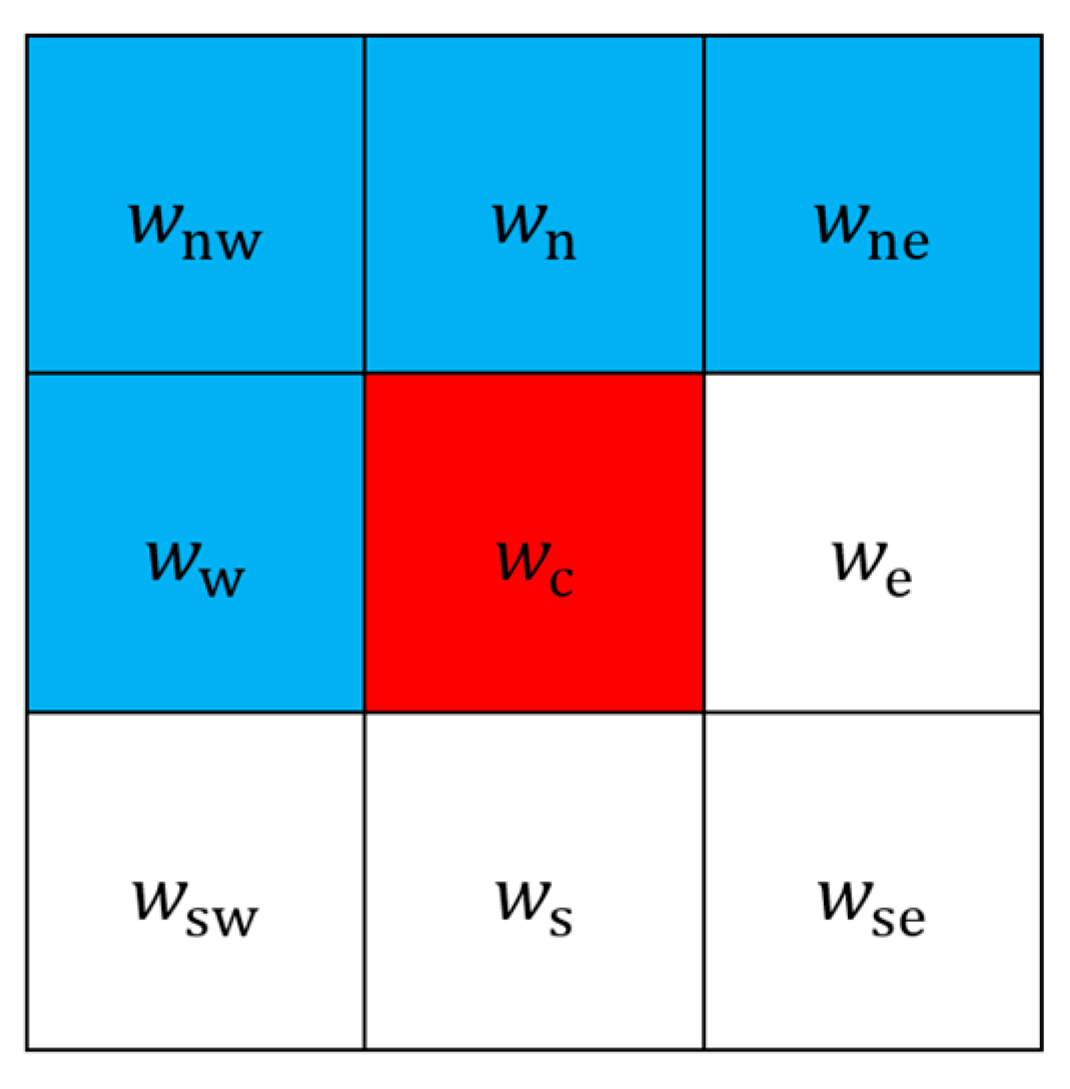
We employ calculations with weighted average prediction to produce a predicted image from the original one. In
Figure 2, locations in blue are served as a mask for performing prediction. The four weight factors in the upper-left (northwest), upper (north), upper-right (northeast), and left (west) side, represented by
,
,
, and
, are trained beforehand. Due to the fact that predicted and original images should look similar, we set the four weights to be positive integers. Predicted luminance value at the center location, or the one in red, can be calculated with a weighted average from the four weight factors in the mask with Equation (3).
By applying the computation when all four weighted pixels are available, the predicted pixels can be determined. With this manner, if we take the original image with the resolution of pixels, there will be predicted pixels produced with Equation (3). The first and the last column, and the first row in the predicted image, are identical to their counterparts in the original image, keeping the same image size between the original and predicted images. With Equation (3), we can present all the pixels in the predicted image as .
Next, we can calculate the difference between
and
, and then generate the difference histogram.
Here,
can be regarded as the difference image, with the difference values ranging from
to
. The smallest and largest difference values in our example are
and
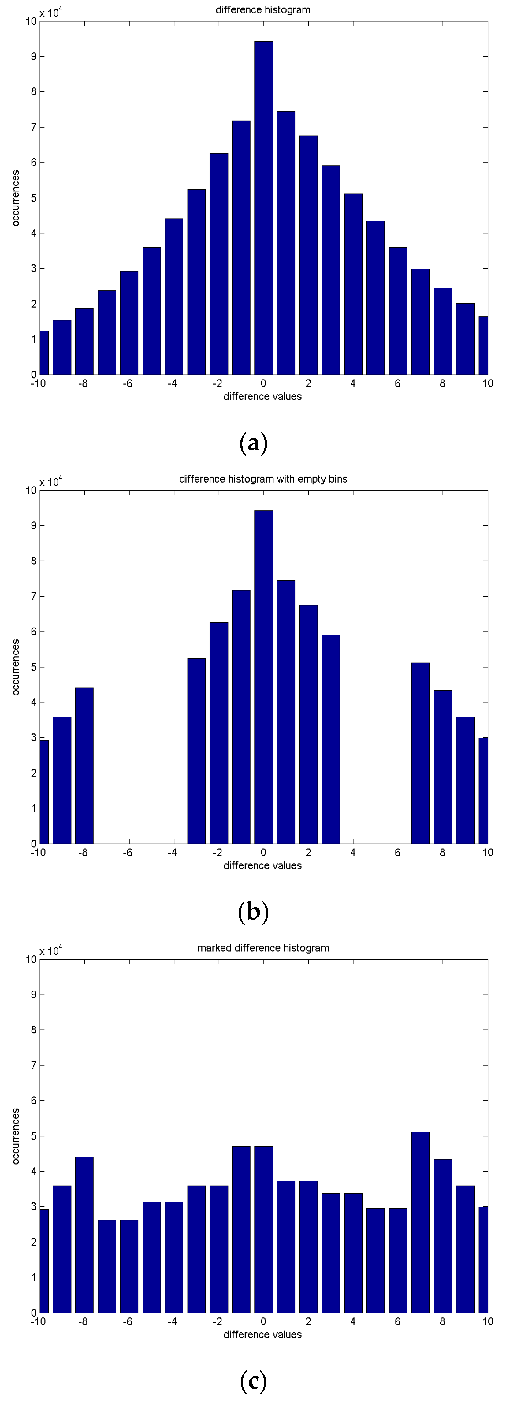
, respectively. We observe that predicted and original images look similar; hence, a large portion of the difference value concentrates are around
. Due to the concentration of difference values around zero, we display the portion between
and
for demonstration purposes in
Figure 3a.
For data embedding, we choose the embedding level (EL), which is a positive integer, and keep the differences between
and
intact. Except for the portions between
and
in the difference histogram, we call the positive ones the right tail, and the negative ones the left tail. We intentionally move the right tail rightward and move the left tail leftward to produce the empty bins in
Figure 3b. With the selected
, we can obtain an emptied difference histogram with Equation (5):
Then, the secret bitstream
can be embedded into the empty bins to produce
Figure 3c. With the embedding of bitstreams, or the composition of random bits, we can obtain a marked difference histogram for the demonstration in Equation (6).
Here,
denotes the secret bit to be embedded. The value of
or
is applied to Equation (6) for data embedding.
We take
Figure 3 as an instance. In
Figure 3, the horizontal axis denotes the difference values in the histogram, and the vertical axis denotes the occurrences.
Figure 3a displays the difference histogram between the original and predicted images, clipped to the range between
and
for better representation.
Figure 3b denotes the emptied bins with Equation (5), for embedding with the condition that
. It implies that there are seven bins, ranging from
to
, or from
to
, that are ready to be modified for data embedding. For embedding binary data, a total of
bins should be prepared. Aside from the existing seven bins that are constrained by
, we need to prepare for an additional seven empty bins, as pointed out in Equation (5) to generate
. Without the loss of generality, we set four empty bins in the negative part, or
to
, and three empty bins in the positive part, or
to
, as depicted in
Figure 3b. The positive difference values larger than
, called the right tail, are intentionally moving rightward by three. At the same time, the negative difference values smaller than
, called the left tail, are intentionally moving leftward by four. These steps produce the emptied difference histogram in
Figure 3b. There might be a very low probability that the difference values may reach both extremes,
or
. The location map [
4] should be provided for decoding, to keep the reversibility. In
Figure 3a, the extremes in the difference histogram are
on the lefthand side and
on the righthand side. Therefore, no overflow problem can be observed.
After that, for embedding the bit
one at a time, we follow Equation (6) for data embedding by re-assigning the difference values to produce the marked difference histogram
in
Figure 3c.
Finally, the modified difference values are added back to the predicted image to produce the marked image
Figure 3 displays an illustration for prediction-based reversible data hiding. With prediction-based techniques for reversible data hiding, we can expect to embed a much higher capacity for the acceptable degradation of the marked image.

