Article

A Few-Shot SE-Relation Net-Based Electronic Nose for Discriminating COPD

1
School of Mechanical Electrical and Information Engineering, Shandong University, Weihai 264209, China
2
School of Future Technology, Xi’an Jiaotong University, Xi’an 710049, China
3
State Key Laboratory for Manufacturing Systems Engineering, Xi’an Jiaotong University, Xi’an 710049, China
4
School of Electrical Engineering, Guangxi University, Nanning 530004, China
5
Guangxi Key Laboratory of Intelligent Control and Maintenance of Power Equipment, Guangxi University, Nanning 530004, China
*
Author to whom correspondence should be addressed.
These authors contributed equally to this work and should be considered co-first authors.
Sensors 2025, 25(15), 4780; https://doi.org/10.3390/s25154780
Submission received: 1 July 2025 / Revised: 31 July 2025 / Accepted: 1 August 2025 / Published: 3 August 2025
(This article belongs to the Special Issue Nature Inspired Engineering: Biomimetic Sensors (2nd Edition))

Abstract

We propose an advanced electronic nose based on SE-RelationNet for COPD diagnosis with limited breath samples. The model integrates residual blocks, BiGRU layers, and squeeze–excitation attention mechanisms to enhance feature-extraction efficiency. Experimental results demonstrate exceptional performance with minimal samples: in 4-way 1-shot tasks, the model achieves 85.8% mean accuracy (F1-score = 0.852), scaling to 93.3% accuracy (F1-score = 0.931) with four samples per class. Ablation studies confirm that the 5-layer residual structure and single-hidden-layer BiGRU optimize stability (h_F1-score ≤ 0.011). Compared to SiameseNet and ProtoNet, SE-RelationNet shows superior accuracy (>15% improvement in 1-shot tasks). This technology enables COPD detection with as few as one breath sample, facilitating early intervention to mitigate lung cancer risks in COPD patients.

1. Introduction

Lung cancer is a highly lethal malignancy that originates from bronchial mucosa or glands. Only 15% of patients are diagnosed in the early stage, while 85% are diagnosed at an advanced stage [1,2,3]. Late diagnosis is often due to similar symptoms with viral diseases, leading to a high mortality rate of around 90% [4]. Early detection is crucial in reducing mortality rates, making cancer prevention and detection significant research topics.
Chronic obstructive pulmonary disease (COPD) is one of the top ten non-infectious diseases worldwide. It is a chronic inflammatory lung disease that causes obstruction in the airflow from the lungs [5]. Research indicates that approximately 1% of COPD patients develop lung cancer annually [6]. Moreover, published studies [7,8] have demonstrated that COPD can serve as a critical and reliable predictor for screening lung cancer risk. The validity of this finding was confirmed by the COPD Lung Cancer Screening Score (COPD-LUCSS), which exhibited a strong correlation between COPD and lung cancer risk.
Several methods have been proposed for testing chronic obstructive pulmonary dis-ease (COPD), including gas chromatography–mass spectrometry (GC-MS) [9,10], spirometry [11,12,13], sputum cytometry, chest radiography [14], and fluoroscopic bronchoscopy. Despite their established roles, each method presents significant limitations. These drawbacks include requirements for specialized personnel, complex and time-consuming procedures, high associated costs, and in some cases, patient invasiveness. Recently, electronic nose (E-nose) applications have emerged as a promising alternative, offering a comparatively easy and fast approach for detecting COPD [15]. Table 1 summarizes the key characteristics and limitations of the mentioned COPD detection methods compared to the emerging electronic nose technology.
The electronic nose (E-nose) is a tool designed to simulate the structure and operation of the human nose, which can assist or replace humans in gas research [16]. It comprises three parts: a sensor array, signal processing, and pattern recognition, which together simulate the biological olfactory system’s response to odor. In recent years, e-noses have supported remarkable achievements in medical diagnosis [17,18,19], environmental monitoring [20,21], food safety [22,23,24], and intelligent agriculture [25,26,27]. Selecting appropriate sensors can ensure that the electronic nose accurately captures the signal characteristics of the target gas [28], while designing excellent pattern recognition algorithms can efficiently utilize these features to significantly enhance the performance of the electronic nose [29]. To enable e-noses to have anthropomorphic or even surpass human gas analysis capabilities, researchers must continuously explore effective gas-recognition algorithms to adapt to various research contexts. In the field of gas classification and concentration prediction, the feasibility of traditional machine learning models such as support vector machine (SVM) [30], XGBoost [31], kernel principal component analysis (KPCA) [32], random forest [33], and deep learning models such as convolutional neural network (CNN) [34] and long short-term memory (LSTM) [35] has been demonstrated one after another.
Current research on e-noses tends to combine long-term data collection with machine learning or deep learning for high performance, although this requires a large number of gas samples for training and a fixed e-nose device. Using too few samples for training can cause overfitting, while using a different sensor array risks bias in the results obtained from the model trained on the old device. Collecting a large number of breath samples is costly for medical institutions, and models trained with many samples can only be used on a specific device, making widespread e-nose use for COPD detection challenging.
Humans can learn new things quickly and accurately with only a few samples. For instance, a person who smells jasmine once can recognize the scent very easily due to their prior knowledge from other experiences. The idea behind FSL is to leverage prior knowledge and train a model with only a small number of samples when faced with a new task. FSL can solve problems such as traditional machine learning algorithms overfitting due to limited data and the inability to directly use deep neural networks and other algorithms that require large amounts of labeled data due to difficulties in labeling or noise. In recent years, FSL based on metric learning has rapidly developed in computer vision and natural language processing. The strategy is to learn prior knowledge to calculate similarities between any two samples and classify unknown samples. Various methods have been proposed, including siamese networks (SiameseNets) [36], matching networks (MatchingNets) [37], prototypical networks (ProtoNets) [38], and Relation Networks (RelationNets) [39], achieving better results in different tasks. Using FSL for e-nose detection enables the device to determine if a new sample is from a COPD patient by training a deep learning network with only a small number of breath samples, promoting the application of e-nose detection for COPD.
In this paper, we construct a model called SE-RelationNet based on the idea of metric learning, and the research performed is as follows: (1) Construct a relational network with residual blocks and bi-directional gate recurrent unit (BiGRU) blocks as the main body, and add squeeze–excitation blocks (SEblock) to improve the performance of the model. (2) Learning prior knowledge from a common gas dataset and solving the problem of detecting patients’ breath in COPD under small-sample situations.
The article outlines the experimental configuration and gas-sampling method in Section 2, introduces the proposed SE-RelationNet in Section 3, discusses the performance of the experiments in Section 4, performs ablation and contrast experiments in Section 5, and concludes in Section 6.

2. Materials and Environments

FSL requires learning problem-solving experience from prior knowledge, with the dataset providing this knowledge referred to as the meta-training set and the dataset used for solving the problem known as the meta-testing set. To ensure compatibility with the same neural network, samples from both sets need to be transformed into the same format before being fed into the model. Generally, the meta-training set should contain more categories to represent prior knowledge, and the meta-training and meta-testing sets should strongly correlate for better transferability [40].
To tackle the challenge of screening COPD patients using only a limited number of labeled breath samples, appropriate selection of the meta-training and validation sets is crucial. Selection criteria include the use of a gas sensor-array collection, with each sample containing the process of starting and stopping the flow of the target gas, and the transformation of both datasets into the same shaped matrix during preprocessing. We chose the “Gas sensor arrays in open sampling settings Data Set” [41] as the meta-training set, containing samples of over 10 common gases collected under normative conditions. Meanwhile, we selected the “Electronic nose dataset for COPD detection from smokers and healthy people through exhaled breath analysis,” including a range of breath samples from COPD patients, general population, smokers, and air samples [42]. These samples can simulate scenarios with very few labeled samples (1–4 per class), where traditional machine learning methods may lead to overfitting. Thus, small-sample learning methods are required in such cases. The two datasets have different collection methods, data formats, and sensor arrays, demonstrating the generality of the model with less stringent requirements for sensor arrays and collection methods. In the following, we will briefly describe these two datasets and illustrate the preprocessing methods.

2.1. Meta-Training Set

The meta-training dataset was sourced from the UCI Machine Learning Repository and was curated by Alexander Vergara et al. For a comprehensive understanding, please refer to paper [43]. This dataset was gathered using an array of 72 sensors, organized into nine groups, within a turbulent wind-tunnel environment infused with various gases. To identify the most discriminative sensors, we implemented a mutual information (MI)-based feature-selection approach evaluating both static and dynamic response characteristics. Mutual information quantifies the dependency between sensor features and gas categories. For a discrete feature X (e.g., Xmean or Xslope and class label Y, it is computed as:
MI ( X ; Y ) = y Y x X p ( x , y ) log p ( x , y ) p ( x ) p ( y )
where p(x,y) is the joint probability distribution, and p(x), p(y) are marginal distributions. Higher MI values indicate stronger relevance for classification. Continuous features were discretized using histogram binning (20 bins) to enable probability estimation. For each sensor, temporal average response Xmean) captured static properties while maximum instantaneous slope (Xslope = max | data|) quantified dynamic sensitivity. Sensors were ranked by combined MI score MI combined , with the top eight sensors selected based on their discriminative power for gas classification tasks. The MI combined is computed as:
MI combined = 1 2 MI ( X mean , Y ) + MI ( X slope , Y )
Detailed information regarding the placement, type, contribution score, and specific gas sensitivities of these sensors is provided in Table 2.
The arrangement of the study involved altering the horizontal distance between the gas source and the sensor array. Data was collected for 11 different gases at six varying distances, with the sensors functioning under five distinct operational conditions. Additionally, the wind speed within the tunnel was modified to three separate levels. Each experimental configuration was subjected to 20 repetitions, and for each repetition, sensor data was logged at a 10 ms interval across a total duration of 400 s, resulting in 40,000 data points per sample.
To ensure stable sensor readings, the wind tunnel was initially flooded with pure air for the first 20 s. Subsequently, the experimental gas was introduced from the 20 s mark until 200 s. From 200 to 400 s, the tunnel was once again ventilated with pure air to cleanse the system. A visual representation of the gas release over time is depicted in Figure 1. Through this methodology, a comprehensive dataset comprising 1800 samples for each gas type was amassed.
During the preparation of the meta-training set, samples with missing data were discarded to maintain the integrity of the dataset. This step was crucial to align the shape of the meta-training set with that of the meta-testing set for effective few-shot learning (FSL). To condense the data, the recordings from each sensor were averaged per second, resulting in 100 data points per second. This reduction led to each sample being represented as a [400, 8] matrix, reflecting 400 s of data from eight sensors. To extract the most pertinent time-series information, the data window was further narrowed down to the segment spanning from 17 to 257 s. This truncation provided a refined sample representation in the form of a [240, 8] matrix, capturing the essential trends in sensor response.
The finalized meta-training set includes 11 gas classes, each uniquely identified by name, molecular formula, concentration, and the number of samples collected, as listed in Table 3.

2.2. Meta-Testing Set

Our meta-testing set was obtained from Mendeley Data, collected and produced by Cristhian Manuel et al. Refer to their paper for more details. The dataset was created to aid the diagnosis of chronic obstructive pulmonary disease and contains four categories of samples: breath of COPD patients (COPD), breath of smokers (SMOKERS), breath of healthy people who do not smoke (CONTROL), and air (AIR). The number of samples in each category is shown in Table 4.
A sensor array of eight sensors was used, with each sample collection involving the subject blowing into the gas while the sensors collected 500 sets of data per second for a total duration of 8 s. This resulted in a matrix of shape [4000, 8], which provided a more complete picture of the approximate trend of the sensor response changes. For each type of sample, we drew a variation curve of the average value of the response of each sensor, as shown in Figure 2.
To ensure that the meta-testing set had the same sample shape as the meta-training set, we used the equal time-interval extraction method to extract 240 out of 4000 recording points. This allowed us to obtain a matrix with a shape of [240, 8].

2.3. Experimental Environment

This experiment was conducted using Python v3.9 and implemented on the PyTorch (v1.13.0) deep learning framework. All models were computed using CUDA with a version of 11.7 for optimized performance.

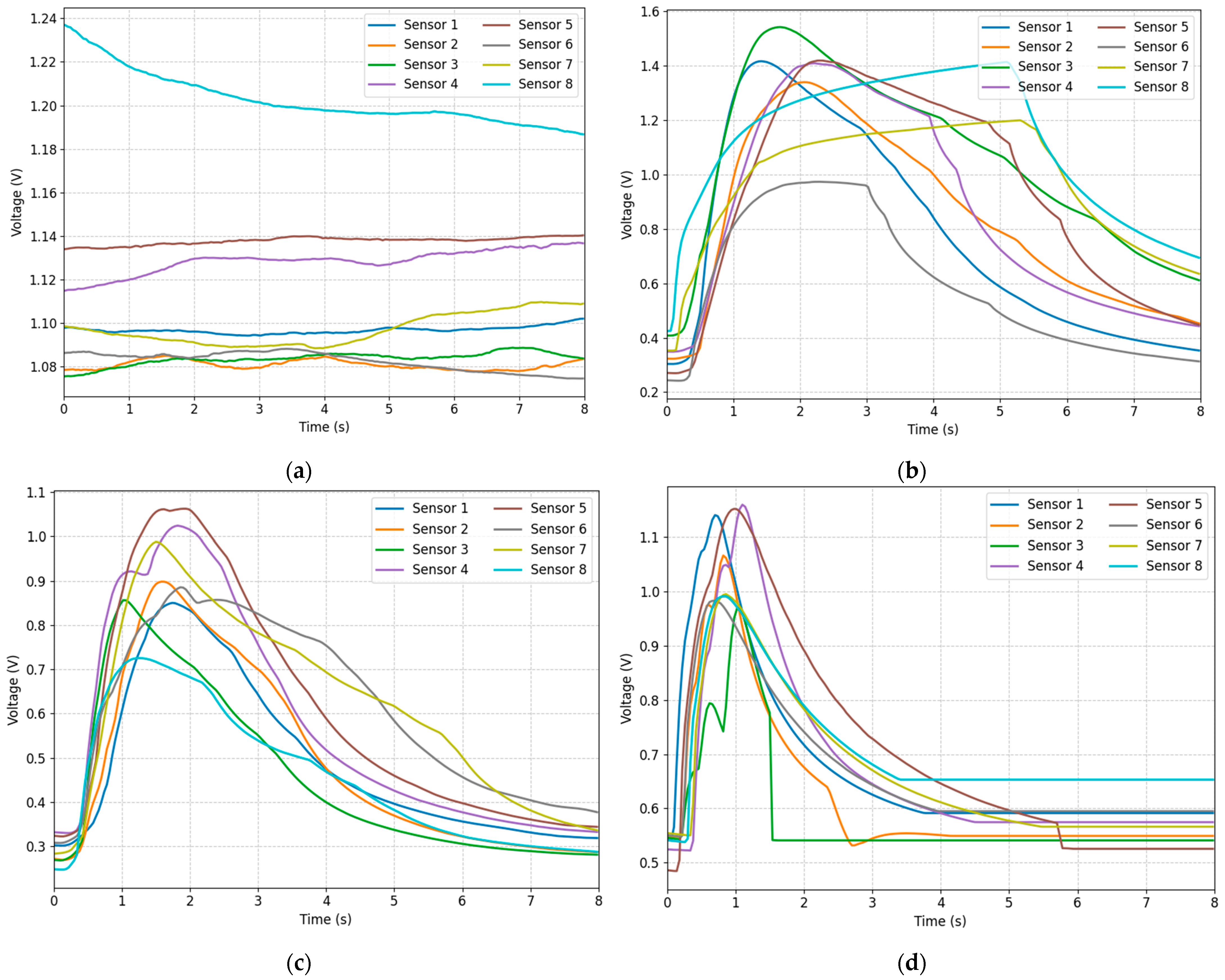
2.4. Signal Preprocessing

To enhance the robustness and generalization ability of the model, we performed the following signal-preprocessing steps:
(1)
Normalization: First, we normalized all sensor data to make them have the same scale. This eliminates the differences in response intensities between different sensors and makes the model more sensitive to the range of input data.
(2)
Channel Shuffling: During each training round, we randomly shuffle and rearrange the sensor channels for all samples within the batch. This aims to prevent the model from over-relying on a specific channel order, thereby enhancing its ability to calculate similarity under different channel orders. Essentially, this is a data augmentation technique that increases the number of training samples and enables the model to learn more generalizable feature representations.

3. Methodology

In this section, we introduce the SE-RelationNet which comprises an embedding module f ϕ and a metrics module g φ . The embedding module extracts sample features using a deep network structure, while the metrics module calculates similarity between two feature matrices. Section 3.1 explains how to use this network for few-shot learning, Section 3.2 covers the embedding module, and Section 3.3 discusses the metrics module.

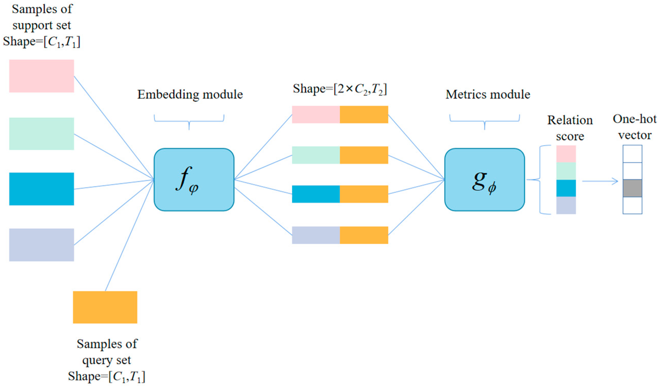
3.1. Training Method of SE-RelationNet

The overall structure of the SE-RelationNet is illustrated in Figure 3. To tackle the few-shot classification task, the model is trained using the N-way K-shot method. Specifically, N classes are selected and K samples are randomly drawn from each class to construct the support set S = x i , y i i = 1 m ( m = K × N ) . Then, P samples are drawn from the remaining part of each category to construct the query set Q = x j , y j j = 1 n ( n = P × N ) . The training process for K = 1 and K > 1 is explained separately.
i. K = 1. Few-shot learning with K = 1, also known as one-shot learning, involves processing a sample x j ( j = 1 , 2 , , P × N ) in the query set using a sample x i ( i = 1 , 2 , , N ) in the support set through an embedding module f ϕ to obtain features. The feature-merging operator C , then combines the obtained features, resulting in input C x i , x j for the metrics module g φ . This generates a similarity score c i , j between 0 and 1, which represents the similarity of x i with x j .
c i , j = g ϕ ( C ( f ϕ ( x i ) , f ϕ ( x j ) ) ) , i = 1 , 2 , , N
ii. K > 1. In the K-shot case with K > 1, the embedding module averages the samples of each class in the support set to obtain the features for that class. The resulting features for each class are then combined with the samples in the query set and input into the metrics module. The metrics module then outputs similarity scores between the samples in the query set and each class of samples in the support set.
To train the model, we use mean square error (MSE) loss, which is typically used for regression problems that resemble classification problems in the label space {0,1}. However, since our model predicts similarity scores, the problem can also be viewed as a regression problem, as shown in the following equation:
ϕ , φ arg min ϕ , φ i = 1 m j = 1 n ( r i , j 1 ( y i = = y j ) ) 2
Once the model is trained with multiple randomly generated tasks, it can determine the degree of similarity between any two samples to a certain extent. During the testing session, the N-way K-shot task is performed several times on the meta-testing set. The class with the highest degree of similarity to the unknown class of samples is selected as the class for that sample, and the model is evaluated using metrics such as accuracy rate.

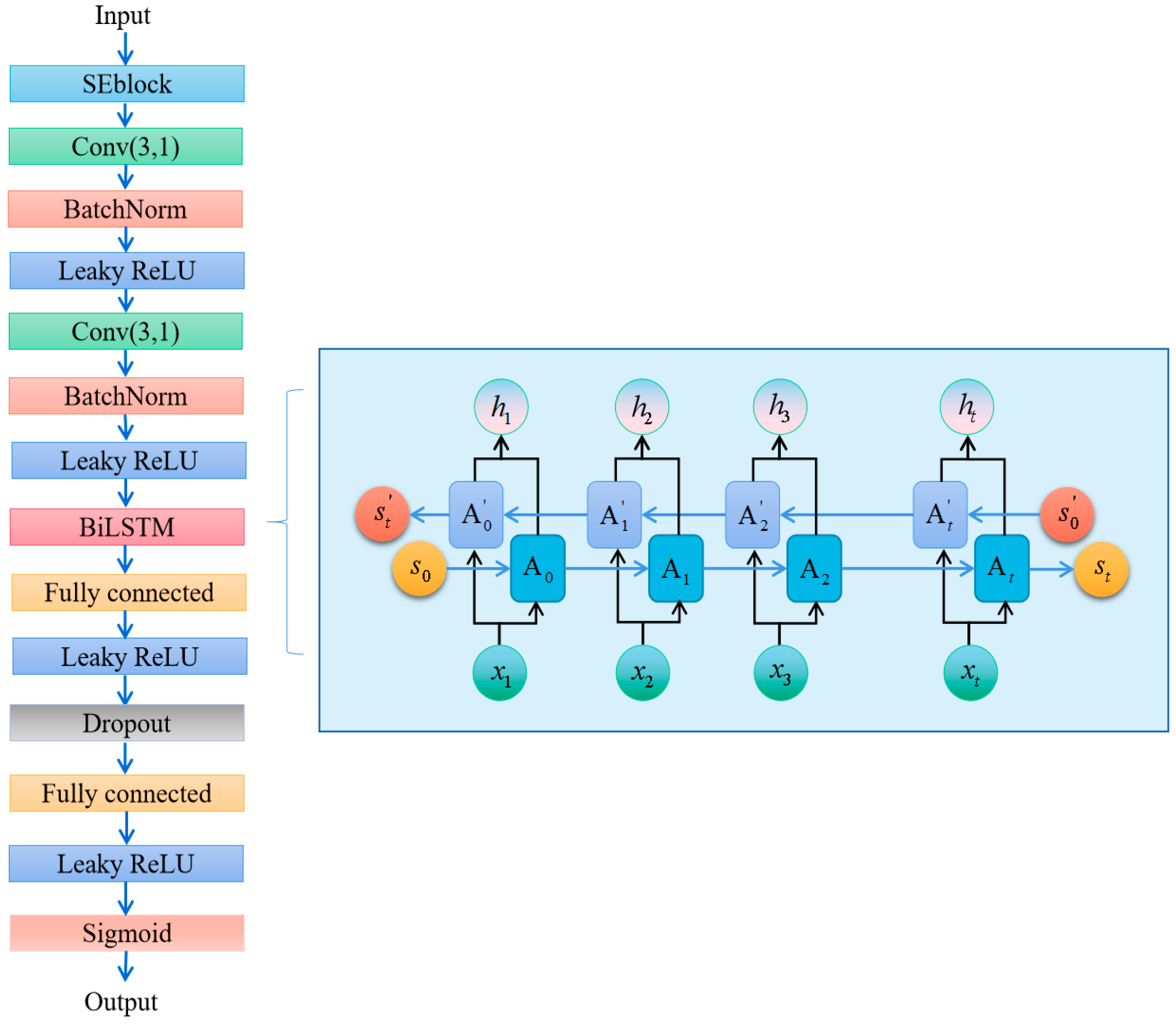
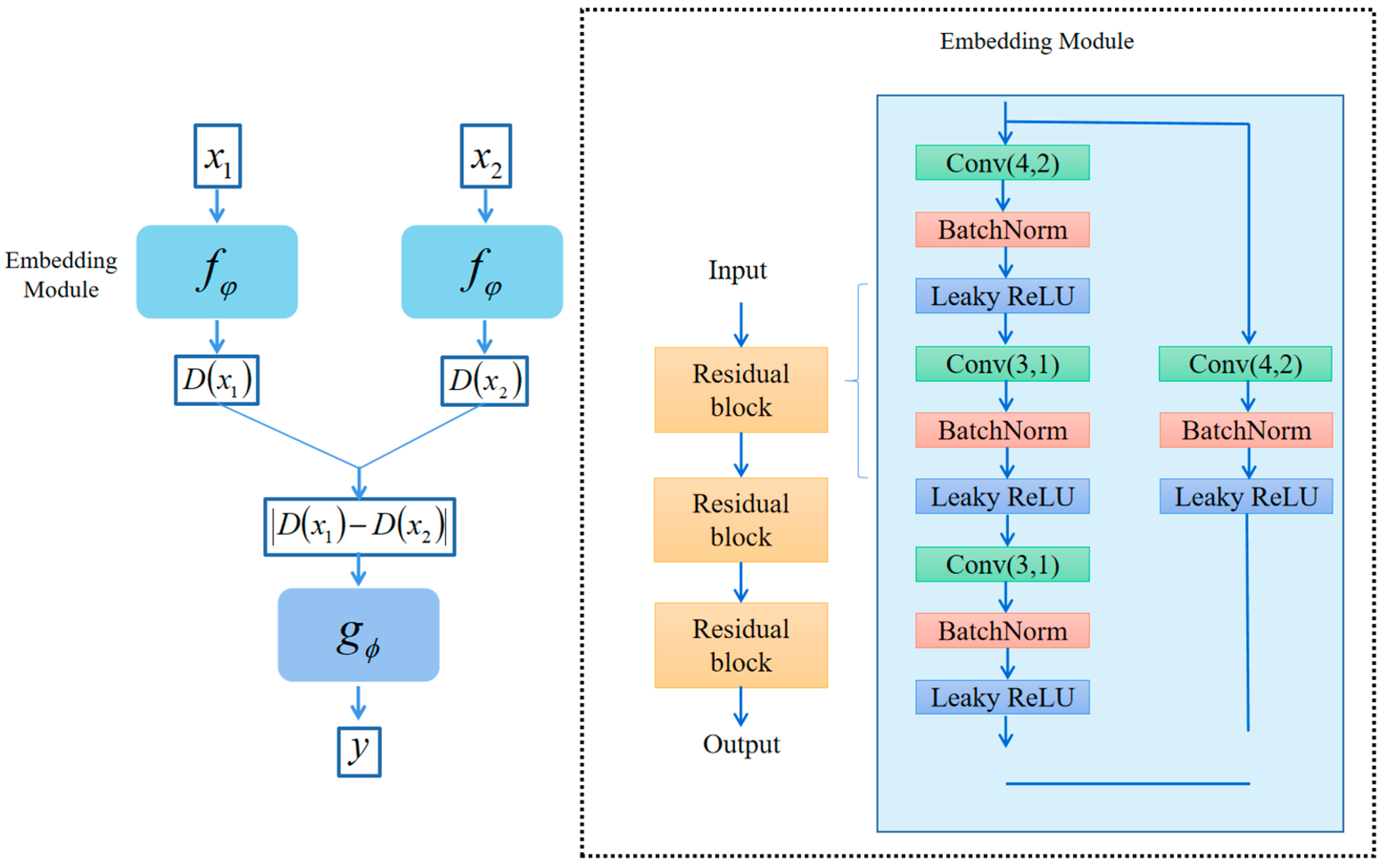
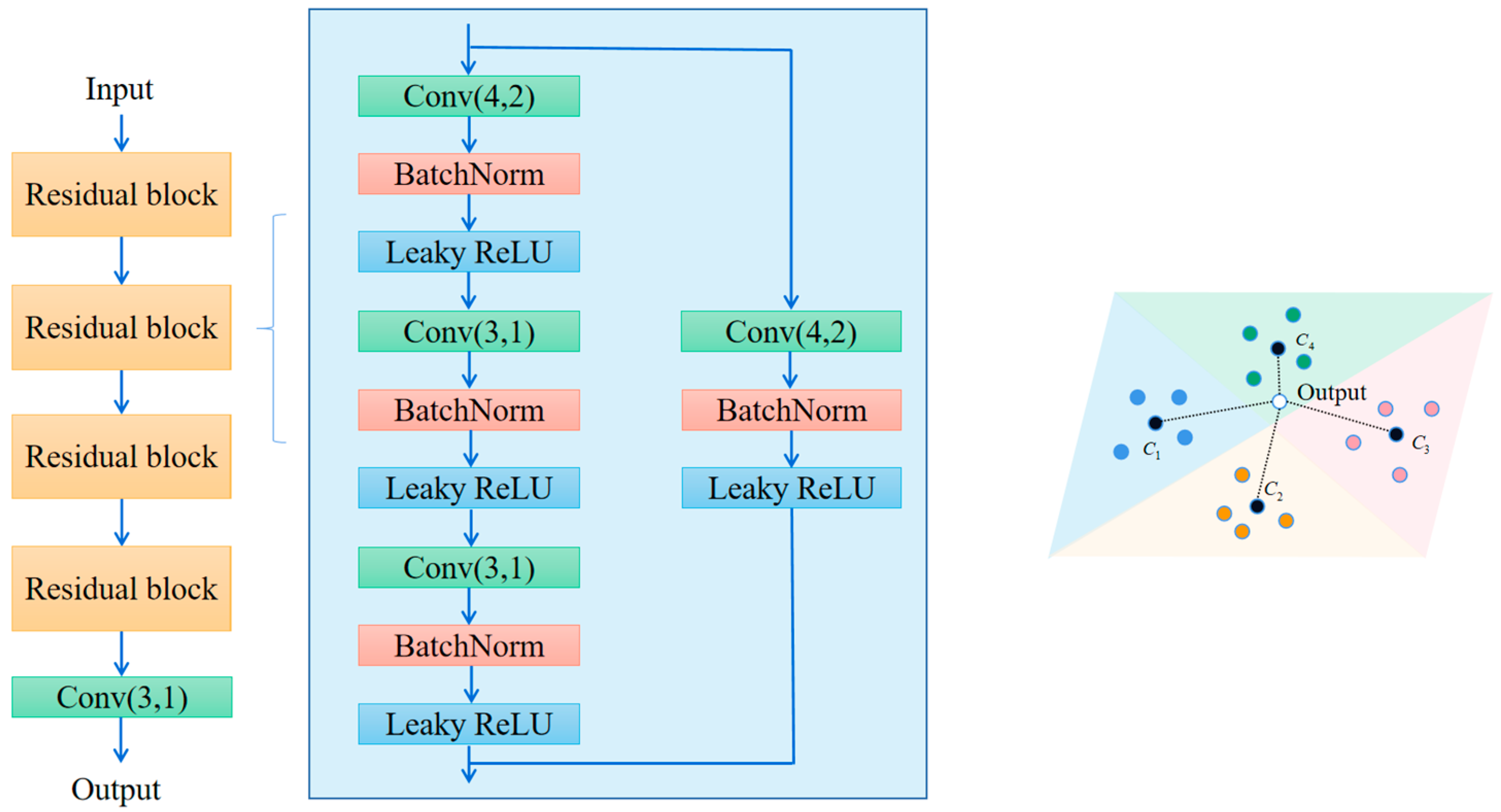
3.2. Embedding Module
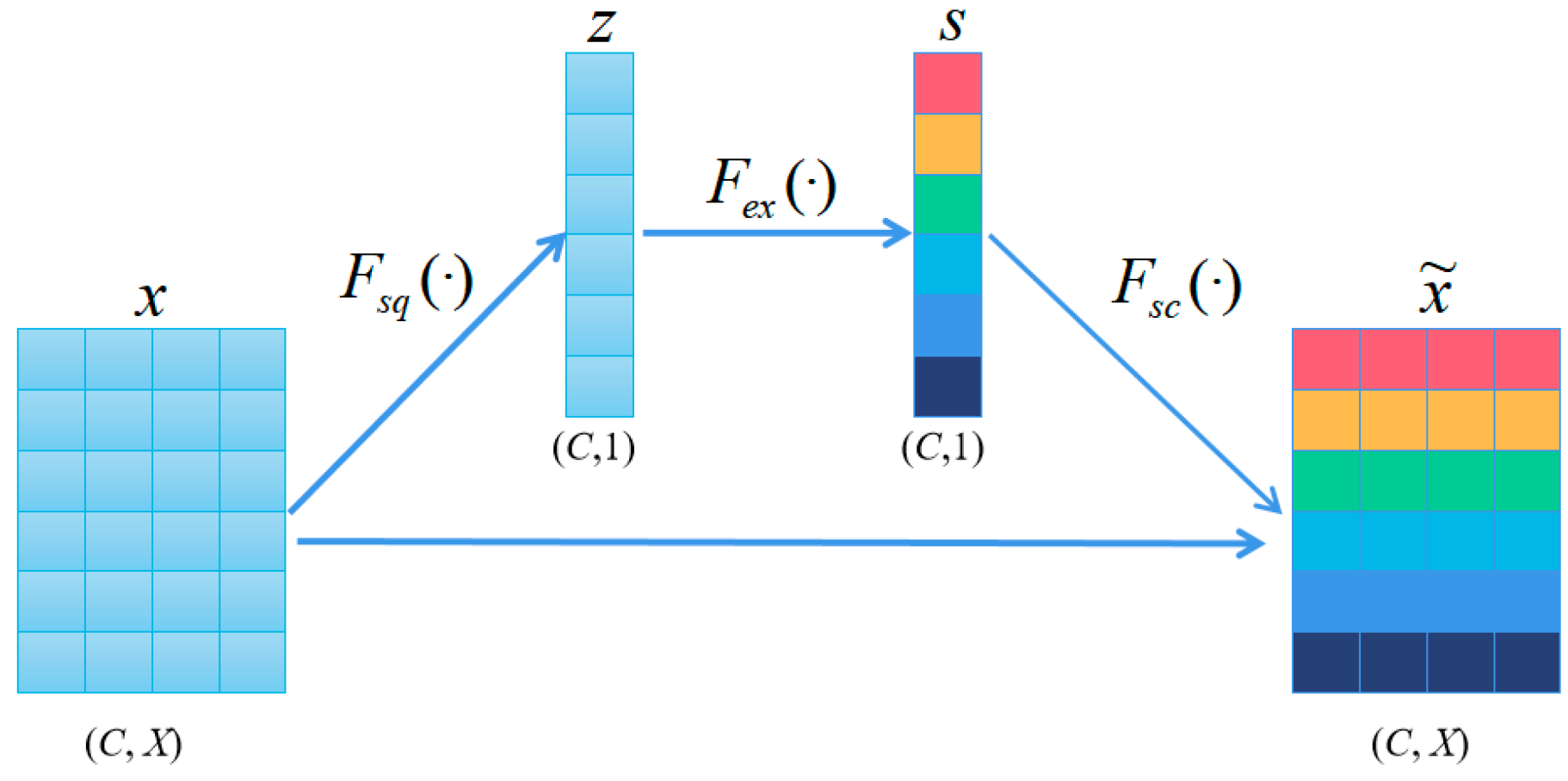
The embedding module is the first module through which the sample data passes. Whether it is a meta-training set sample or a meta-testing set sample, it is in the form of a matrix with the shape [240, 8], representing the data recorded by 8 sensors at 240 recording points. The embedding module extracts abstract features from this time series for further processing by the metrics module. Its output is a matrix with the shape [63, 30]. Figure 4 depicts the structure of the embedding module.
The ability of a neural network to extract abstract features improves with increasing depth. However, a network that is too deep can suffer from gradient dispersion and gradient explosion. Traditional solutions such as normalized initialization and batch normalization may slow down the original problem to some extent, but they introduce new problems. One of these problems is the degradation of network performance. Kaiming He proposed residual blocks as an effective solution to this problem. Hence, we added three residual blocks to our network [44].
Each residual block comprises pathway F 1 and pathway F 2 . Pathway F 1 includes three convolutional layers and one SEblock, while pathway F 2 consists of only one convolutional layer. Assuming that x is the input of the residual block and y is the output, w 1 and w 2 are the parameters of pathway F 1 and pathway F 2 , respectively, which are also the objects we need to optimize. The equation below shows the relationship between the input and output:
y = F 1 ( x , w 1 ) + F 2 ( x , w 2 )
During backpropagation, gradient fading may occur if the pathway between layers is too long. However, using a shorter pathway F 2 can mitigate this issue by propagating gradients across fewer layers. Leaky ReLU is a modified linear activation function with f(x) = max (ax, x), where a < 1 (usually set to 0.01). It has better convergence and generalization capabilities compared to traditional ReLU and can improve the accuracy and stability of deep neural networks. When a value of 0.01 is used for parameter a, the shapes of the leaky ReLU function and the ReLU function can be plotted as illustrated in Figure 5.
In the network, we incorporated the SEblock, an attention mechanism illustrated in Figure 6, to enhance its performance [45]. The SEblock selectively emphasizes informative features by adaptively recalibrating them based on their relevance. The basic idea is as follows:
(1)
Squeeze (Fsq). Aggregates the features of each channel by averaging pooling:
z c = F s q ( x c ) = 1 X i T x c ( i )
Here, zc is the compressed channel vector, xc is the c-th channel of the input feature map, and T is the dimension of each channel.
(2)
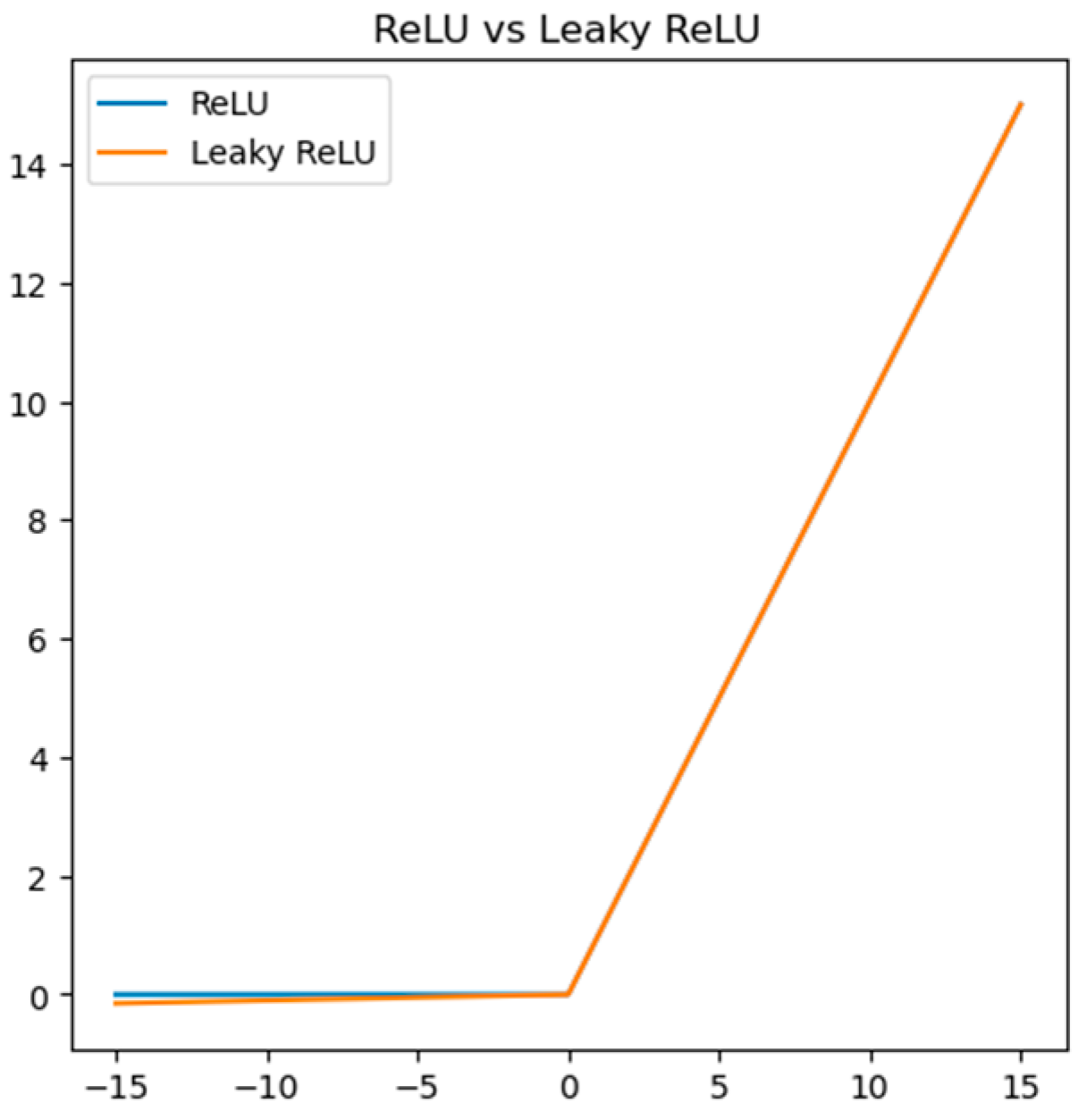
Extraction (Fex). The compressed vectors undergo two fully connected layers to produce channel weights. To improve computational efficiency, we set a reduction factor r a t i o and halve the number of neurons in the first layer by 1 r a t i o while using ReLU as a nonlinear function. The second layer has the same number of neurons as the input and applies the sigmoid function to confine the weights between 0 and 1. These fully connected layers are parameterized by w 1 and w 2 .
s = F e x ( z ) = f 2 ( f 1 ( z , w 1 ) , w 2 )
Here, f1 and f2 are two consecutive fully connected layers used to process. This step enables SEblocks to use the global information of each channel and selectively emphasize the channel features.
(3)
Scale (Fsc). The importance score of each channel is obtained from the “Extraction“ stage, which we use to reweight the channels. This involves sequentially multiplying each channel with its corresponding weight to produce the calibrated attention channels.
x ˜ c = F s c ( x c , s c ) = s c x c

3.3. Metrics Module

To obtain the similarity between unknown and known category samples, we concatenate them and input them into the “metrics” module illustrated in Figure 7. The metrics module consists of a convolutional layer for abstract feature extraction, BiGRU blocks (a variant of GRU for time-series feature extraction), SEblock for improved expressiveness, and a fully connected layer to process the output data from the BiGRU block. Finally, the sigmoid function is applied to the output to produce a probability score between 0 and 1, indicating the predicted category of the unknown sample.
The BiGRU block, illustrated in Figure 7, introduces the concept of hidden state to extract time-series features by learning the information at each moment and combining it with the information before and after [46]. Compared to traditional fully connected layer networks, this results in improved feature-extraction performance. The input–output relationships for each layer can be expressed as follows:
r t = f ( W r x t + U r h t 1 + b r )
This calculates the “reset gate” value. It decides how much of the past hidden state ht−1 to forget or reset based on the current input xt. A value close to 0 means discarding most past information, while a value close to 1 means retaining it. This helps the model ignore irrelevant historical data when processing new inputs.
z t = f ( W z x t + U z h t 1 + b z )
This computes the “update gate” value. It determines how much new information from the current input should update the hidden state. For example, if zt is near 1, the hidden state relies heavily on past values; if near 0, it prioritizes new inputs. This gate balances between retaining long-term memory and incorporating fresh data.
h t = tan h ( W h x t + U h ( r t h t 1 ) + b h )
This generates a “candidate” for the new hidden state. It combines the current input xt with a filtered version of the past hidden state (using the reset gate rt). The tanh function ensures the output is normalized, preventing extreme values. Essentially, this step proposes a new state based on selective past and current information.
h t = z t h t 1 + ( 1 z t ) h t
This produces the final hidden state ht by blending the previous hidden state ht−1 and the candidate h t , using the update gate zt as a weighting factor. If zt is high, the state leans toward history; if low, it favors the new candidate. This allows the BiGRU to adaptively learn sequential patterns, such as trends in breath sample responses.
To optimize model performance, we set the number of hidden layers in the BiGRU block to 1.

4. Experiments and Analysis

In this section, we begin by setting appropriate parameters for the SE-RelationNet and assessing its performance.

4.1. Parameter Optimization of the SE-RelationNet

SE-RelationNet’s training benefits from setting optimal parameters for improved accuracy and faster convergence. The trial-and-error method is used to select the best parameters, which are listed in Table 5 for easy replication of the model.

4.2. Selection of Evaluation Indicators

To evaluate the SE-RelationNet model, we used four metrics: mean_accuracy, h_accuracy, mean_F1-score, and h_F1-score. Additionally, we employed a confusion matrix as a common visualization tool for supervised learning, which can be seen in Table 6.
The formula for accuracy, which is the most commonly used evaluation metric for classification tasks, is as follows:
a c c u r a c y = T P + T N T P + T N + F P + F N
The F1-score is a reconciled mean of precision and recall, proposed as a more robust indicator than accuracy due to susceptibility to sample equilibrium. Its formula is:
p r e c s i o n = T P T P + F P
r e c a l l = T P T P + F N
F 1 s c o r e = 2 × p r c e s i o n × r e c a l l p r e c s i o n + r e c a l l
For each round the model is trained, we will test the model using a meta-test set, and each test yields accuracy and F1-score. Let the n different accuracy’s obtained be a 1 , a 2 , …, a n , and the n different F1-scores are f 1 , f 2 , …, f n . To accurately measure the model effect, we take the average of these two metrics separately:
For each training round, the model is tested on a meta-test set to obtain accuracy and F1-score. Let the n different accuracy scores be a 1 , a 2 , …, a n , and the n different F1-scores be f 1 , f 2 , …, f n . To accurately measure the model’s effectiveness, we calculate the average of these two metrics separately:
m e a n _ a c c u r a c y = 1 n i = 1 n a i
m e a n _ F 1 s c o r e = 1 n i = 1 n f i
To assess the dispersion of a 1 , a 2 , …, a n , we assume that they follow a t-distribution and introduce the distance h_accuracy, which represents the distance between the right endpoint of the 95% confidence interval and the mean_accuracy. The formula for calculating h_accuracy is as follows:
h _ a c c u r a c y = s e m x
s e m = σ n
where sem and σ are the standard error and standard deviation of n accuracy, respectively, and x are the positions of the right end quantile of the t distribution at a confidence level of 95% and a degree of freedom of n − 1. h_accuracy is calculated in the same way as h_F1-score. When mean_accuracy and mean_F1-score are larger, the stronger the ability of the model to predict correctly. The smaller the h_accuracy and h_F1-score values, the higher the confidence level of the model and the less randomness present in the model performance due to training.
For every 20 epochs trained by the model, we conduct a test containing 50 epochs on the meta-testing set (each epoch consisting of randomly divided N-way K-shot tasks) to obtain accuracy and F1-score. Figure 8 shows a line graph with epoch as the horizontal axis and accuracy or F1-score as the vertical axis. The graph indicates that both metrics exhibit an overall upward trend until the 600th epoch, after which they fluctuate around a certain value.
Select the records between 700 and 1000 epochs with accuracy and F1-score to find their indicators as shown in Table 7.
Table 7 shows that mean_accuracy and mean_F1-score increase with increasing K when there is no clear trend in the metrics. However, this increasing trend is not significant when K is greater than 1. This suggests that increasing K within a certain range can improve the model’s effectiveness, but using a larger K implies a larger sampling scale, which may not necessarily lead to better results beyond a certain point.
The marginal improvement from K = 1 to K = 4 stems from the inherent properties of the learned embedding space and the metric mechanism. Our model focuses on extracting abstract feature representations (or “class prototypes”) through the embedding module, with K primarily influencing the robustness of prototype construction during metric comparison.
(1)
K = 1 performance: The strong baseline accuracy (e.g., >0.85 mean_F1-score in 4-way tasks) indicates effective generalization, as a single sample suffices to capture core class characteristics. However, individual sample noise or outliers can degrade prototype fidelity.
(2)
K > 1 refinement: Increasing K averages out noise and incorporates diverse sample variations, enhancing prototype stability. This explains the gradual accuracy rise up to K = 4.
(3)
Asymptotic behavior beyond K = 4: Once K exceeds a threshold (~4 in our experiments), prototypes saturate in representational quality. Further samples yield diminishing returns, as the embedding space already encodes class-discriminative features efficiently.
This phenomenon mirrors human cognition: recognizing a new object after one exposure (K = 1) is possible but error-prone; repeated exposures (K > 1) refine mental prototypes until stability is achieved. Thus, the limited K-scaling gain validates the embedding space’s optimality—a few samples suffice for near-peak generalization.

5. Results and Discussion

In this section, we performed ablation experiments to identify the optimal number of residual block layers, assess the suitability of BiGRU blocks, and evaluate the effectiveness of the attention mechanism. Additionally, we included two few-shot learning models as controls for the proposed model.

5.1. Making Changes to the BiGRU Block

To investigate the rationality of the BiGRU with a single hidden layer, we designed control experiments for the BiGRU. The control group replaced the BiGRU with one hidden layer (group 1) with a BiGRU with two hidden layers (group 2), a BiGRU with three hidden layers (group 3), a GRU block with one hidden layer (group 4), a BiLSTM block with one hidden layer (group 5), a RNN block with one hidden layer (group 6), and a LSTM block with one hidden layer (group 7), respectively. To ensure the evaluation reflects the model’s performance at convergence, records between 700 and 1000 epochs were selected for aggregation. This interval was chosen because, as illustrated in Figure 8, the F1-score for all models, particularly SE-RelationNet, exhibited minimal fluctuations and stabilized after approximately 700 training epochs. The calculated mean_F1-score and h_F1-score within this stable period provide a reliable assessment of the model’s generalization capability, as shown in Table 8.
The results show that the BiGRU block with one hidden layer (group 1) consistently outperformed deeper variants (groups 2 and 3) across all few-shot settings (Table 7). This superiority arises primarily from reduced overfitting risk and computational efficiency. Deeper networks introduce more parameters, making them prone to memorizing noise rather than learning generalizable features in the limited-data context of our meta-testing set. The single-layer architecture avoids this degradation and manages gradients more effectively. Furthermore, the bidirectional design (group 1) significantly outperformed the unidirectional GRU (group 4), particularly in the challenging 1-shot task (0.852 vs. 0.816 mean_F1-score), due to its enhanced contextual awareness by processing sequences in both forward and backward directions, capturing complex temporal patterns in sensor responses (Figure 2). While BiLSTM (group 5) showed competitive performance in some tasks (e.g., 4-way 4-shot), the GRU-based model (group 1) generally achieved higher or comparable mean_F1-scores (e.g., 0.852 vs. 0.823 in 4-way 1-shot), making it better suited for our small-sample learning scenario. Therefore, BiGRU with one hidden layer is the best design.
The results show that the BiGRU block with one hidden layer and the convolutional layer outperformed the other structures, but the former showed higher stability compared to the latter. Overall, the BiGRU block with one hidden layer is the better design.

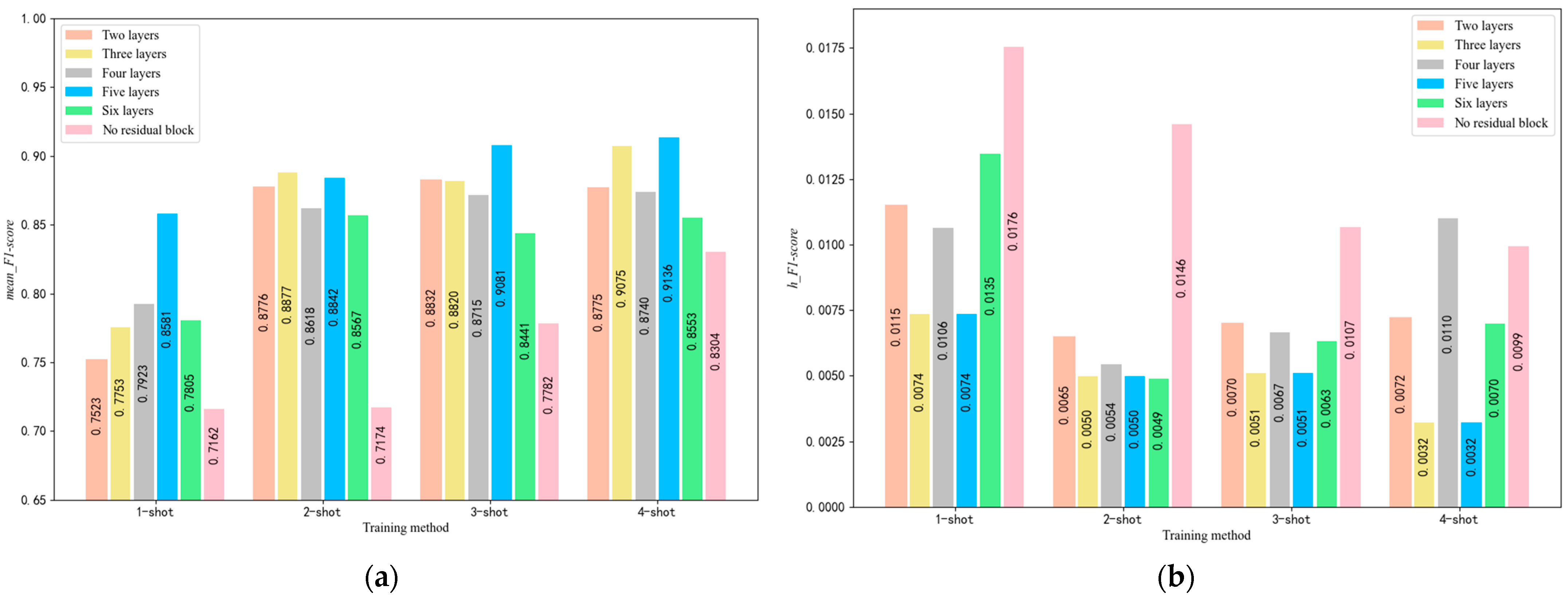
5.2. Selection of the Number of Residual Block Layers

Prof. Kaiming He’s study suggested that the number of layers in the residual block should be at least two, as a single layer would not be meaningful [47]. To examine the suitability of using five layers of residual blocks, we conducted an experiment where we varied the number of layers in the embedding module and selected records between 700 and 1000 epochs to obtain the mean_F1-score and h_F1-score. Additionally, we replaced each residual block with five concatenated convolutional layers to investigate the necessity of using residual blocks. The resulting histogram is shown in Figure 9.
To provide a deeper analysis of the results in Figure 9, we observe that the 5-layer residual block consistently outperforms other configurations across all few-shot tasks (4-way 1-shot to 4-way 4-shot). Specifically, for the 4-way 4-shot task, the mean_F1-score peaks at 0.931 with an h_F1-score of 0.008, indicating not only high accuracy but also exceptional stability. This optimal performance is attributed to the residual blocks’ ability to mitigate gradient vanishing while enabling sufficient depth for feature abstraction. In contrast, fewer layers result in lower mean_F1-scores due to inadequate hierarchical representation learning. Conversely, while not tested beyond five layers, excessive depth (implied by the trend) could increase computational latency and overfitting risks, as seen in the marginal decline in stability for non-residual configurations. Additionally, the reduced h_F1-score for 5-layer blocks underscores their robustness to input variations, which is critical for small-sample COPD detection where data noise is prevalent. This analysis confirms that a 5-layer residual design achieves an optimal trade-off between model complexity and generalization, directly supporting our architectural choice for SE-RelationNet.

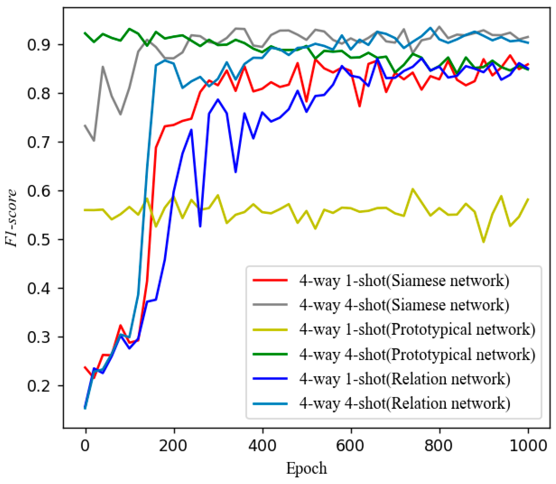
5.3. Control Experiments with Other Models

We chose SiameseNet and ProtoNet as the control networks for SE-RelationNet, which are described below.
The SiameseNet is a basic one-shot learning method that has been adapted to also handle few-shot problems with K > 1. Its structure is shown in Figure 10. The embedding module outputs a feature vector, which is used to compute the similarity between a pair of samples in the query set and support set. This is achieved by averaging the feature vectors of the support set samples and subtracting from the feature vectors of the query set samples. The absolute values are then input to the metrics module, which consists of two fully connected layers, and outputs a number between 0 and 1 representing the similarity of the two samples.
ProtoNet is a few-shot learning method, with the structure shown in Figure 11. K samples of each class in the support set are projected into the Euclidean space by the embedding module, and the average value is taken as the prototypical vector of that class. Samples in the query set are projected by the embedding module, and the Euclidean distance from the prototypical vector of each class is calculated. Finally, the Softmax function is used to evaluate the probability that the samples belong to each category.
The learning rates for SiameseNet, ProtoNet, and SE-RelationNet are 0.0001, 0.00001, and 0.0001, respectively. We selected the F1-score recorded between 700 and 1000 training rounds and calculated the mean_F1-score and h_F1-score. The results are shown in Figure 12.
Figure 12 shows that in the one-shot learning task, the mean_F1-score of both the SiameseNet and the ProtoNet is less than 0.7, while the SE-RelationNet is higher than 0.8. The lower h_F1-score of the SiameseNet and the ProtoNet indicates that they have higher stability; in the one-shot learning task, the SE-RelationNet has higher accuracy and lower stability. In the few-shot learning task with K > 1, the SE-RelationNet has higher accuracy and lower stability, but its stability gets significantly improved as N increases.
The trend of F1-score with epoch for the three models is plotted in Figure 13 under 4-way 1-shot and 4-way 4-shot training methods. Regardless of the training method, the ProtoNet can reach convergence after very few training rounds, while the SiameseNet and the SE-RelationNet need more than 100 training rounds to converge.

6. Conclusions

In this paper, we propose an electronic nose based on SE-RelationNet for identifying COPD patients by analyzing their breath samples when the number of labeled samples is limited. SE-RelationNet consists of an embedding module and a metric module, and we conducted several ablation experiments on its structure to optimize its performance. The results showed that using a 5-layer residual block and a BiGRU block with one hidden layer as the metric module achieved the highest accuracy and stability. Compared to SiameseNet and ProtoNet, our model demonstrated superior performance, achieving a mean accuracy of 93.3% in 4-way 4-shot tasks and outperforming SiameseNet by 15.2% in F1-score under one-shot conditions.
However, two limitations require attention:
(1)
Cross-device generalizability: While SE-RelationNet reduces sensor dependency (Section 2.1 and Section 2.2), performance fluctuations occur when meta-training/meta-testing sensor arrays differ significantly (h_accuracy ≤ 0.010 in Table 7).
(2)
Clinical-scale validation: Current validation used curated public datasets. Real-world clinical trials with diverse patient cohorts are needed to assess robustness against comorbidities like asthma or pneumonia.
Future work will focus on:
(1)
Extending the model to multi-class COPD severity detection (mild/moderate/severe) using VOC profiles, leveraging the COPD-LUCSS risk correlation.
(2)
Integrating lung cancer biomarkers (e.g., aldehyde/ketone signatures) into sensor arrays for joint screening.
(3)
Addressing the above limitations through hybrid sensor-fusion algorithms and multi-center clinical trials.
SE-RelationNet’s relocatability enables researchers to build the e-nose using common sensor arrays, requiring only minimal breath samples (as few as one per class) for COPD detection. This facilitates early lung cancer risk stratification in high-risk COPD populations, ultimately promoting accessible point-of-care diagnostics. To translate COPD discrimination into lung cancer risk stratification, we propose:
(1)
Multi-class COPD subtype detection—Extend SE-RelationNet to classify COPD severity (mild/moderate/severe) using VOC profiles, leveraging the established COPD-LUCSS risk correlation.
(2)
Biomarker integration—Incorporate lung cancer-specific biomarkers (e.g., aldehyde/ketone signatures) into the sensor array, enabling simultaneous COPD/lung cancer screening.
(3)
Hybrid risk modeling—Develop algorithms combining COPD subtypes, biomarkers, and clinical factors to generate quantifiable risk scores.
(4)
Prospective validation—Conduct multi-center trials to validate stratification efficacy prior to clinical deployment.
(5)
This framework bridges the gap between our technology and actionable cancer-prevention strategies.

Author Contributions

Conceptualization, Z.X. and Y.T.; methodology, Y.T.; software, Y.T.; validation, Z.X. and Y.T.; investigation, Y.T.; resources, Y.T.; data curation, Y.T.; writing—original draft preparation, Z.X.; writing—review and editing, Z.X. and Y.T.; visualization, Y.T.; supervision, P.J.; project administration, P.J.; funding acquisition, P.J. All authors have read and agreed to the published version of the manuscript.

Funding

This work was supported by National Natural Science Foundation of China [Grant No. 61906160]; Sichuan Science and Technology Program [Grant No. 2022NSFSC1632].

Institutional Review Board Statement

Not applicable.

Informed Consent Statement

Not applicable.

Data Availability Statement

The data used is from public datasets, and the code will be made public after the paper is accepted.

Conflicts of Interest

The authors declare no conflicts of interest.

References

  1. Ahmad, A.S.; Mayya, A.M. A new tool to predict lung cancer based on risk factors. Heliyon 2020, 2, e3402. [Google Scholar] [CrossRef]
  2. El-Khoury, V.; Schritz, A.; Kim, S.; Lesur, A.; Sertamo, K.; Bernardin, F.; Petritis, K.; Pirrotte, P.; Selinsky, C.; Whiteaker, J.R.; et al. Identification of a blood-based protein biomarker panel for lung cancer detection. Cancers 2020, 6, 1629. [Google Scholar] [CrossRef]
  3. Cainap, C.; Bălăcescu, O.; Cainap, S.S.; Pop, L. Next generation sequencing technology in lung cancer diagnosis. Biology 2021, 9, 864. [Google Scholar] [CrossRef]
  4. Binson, V.A.; Subramoniam, M.; Sunny, Y.; Mathew, L. Prediction of pulmonary diseases with electronic nose using SVM and XGBoost. IEEE Sens. J. 2021, 18, 20886–20895. [Google Scholar] [CrossRef]
  5. Rennard, S.I.; Martinez, F.J.; Rabe, K.F.; Sethi, S.; Pizzichini, E.; McIvor, A.; Siddiqui, S.; Anzueto, A.; Zhu, H. Effects of roflumilast in COPD patients receiving inhaled corticosteroid/long-acting β2-agonist fixed-dose combination: RE2SPOND rationale and study design. Int. J. Chronic Obstruct. Pulm. Dis. 2016, 11, 1921–1928. [Google Scholar] [CrossRef] [PubMed]
  6. Sekine, Y.; Katsura, H.; Koh, E.; Hiroshima, K.; Fujisawa, T. Early detection of COPD is important for lung cancer surveillance. Eur. Respir. J. 2012, 5, 1230–1240. [Google Scholar] [CrossRef]
  7. Mirza, S.; Clay, R.D.; Koslow, M.A.; Scanlon, P.D. COPD guidelines: A review of the 2018 GOLD report. Mayo Clin. Proc. 2018, 93, 1488–1502. [Google Scholar] [CrossRef]
  8. Wilson, D.O.; de Torres, J.P. Lung cancer screening: How do we make it better? Quant. Imaging Med. Surg. 2020, 10, 533–536. [Google Scholar] [CrossRef]
  9. Li, X.O.; Cheng, J.; Shen, Y.; Chen, J.; Wang, T.; Wen, F.; Chen, L. Metabolomic analysis of lung cancer patients with chronic obstructive pulmonary disease using gas chromatography-mass spectrometry. J. Pharm. Biomed. Anal. 2020, 180, 113524. [Google Scholar] [CrossRef]
  10. Bregy, L.; Nussbaumer-Ochsner, Y.; Martinez-Lozano Sinues, P.; García-Gómez, D.; Suter, Y.; Gaisl, T.; Stebler, N.; Gaugg, M.T.; Kohler, M.; Zenobi, R. Real-time mass spectrometric identification of metabolites characteristic of chronic obstructive pulmonary disease in exhaled breath. Clin. Mass Spectrom. 2018, 10, 29–35. [Google Scholar] [CrossRef] [PubMed]
  11. Bodduluri, S.; Nakhmani, A.; Reinhardt, J.M.; Wilson, C.G.; McDonald, M.N.; Rudraraju, R.; Jaeger, B.C.; Bhakta, N.R.; Castaldi, P.J.; Sciurba, F.C.; et al. Deep neural network analyses of spirometry for structural phenotyping of chronic obstructive pulmonary disease. JCI Insight 2020, 5, e134123. [Google Scholar] [CrossRef] [PubMed]
  12. Kim, S.; Oh, J.; Kim, Y.; Ban, H.; Kwon, Y.; Oh, I.; Kim, K.; Kim, Y.; Lim, S. Differences in classification of COPD group using COPD assessment test (CAT) or modified Medical Research Council (mMRC) dyspnea scores: A cross-sectional analysis. BMC Pulm. Med. 2013, 13, 35. [Google Scholar] [CrossRef]
  13. Tinkelman, D.; Price, D.; Nordyke, R.; Halbert, R. Misdiagnosis of COPD and asthma in primary care patients 40 years of age and over. J. Asthma 2009, 46, 75–80. [Google Scholar] [CrossRef]
  14. Akopov, A.; Papayan, G. Photodynamic theranostics of central lung cancer: Present state and future prospects. Photodiagn. Photodyn. Ther. 2021, 33, 102203. [Google Scholar] [CrossRef]
  15. Peng, J.; Mei, H.; Yang, R.; Meng, K.; Shi, L.; Zhao, J.; Zhang, B.; Xuan, F.; Wang, T.; Zhang, T. Olfactory diagnosis model for lung health evaluation based on pyramid pooling and SHAP-based dual encoders. ACS Sens. 2024, 9, 4934–4946. [Google Scholar] [CrossRef]
  16. Shooshtari, M.M.; Salehi, S. An electronic nose based on carbon nanotube-titanium dioxide hybrid nanostructures for detection and discrimination of volatile organic compounds. Sens. Actuators B Chem. 2022, 357, 131418. [Google Scholar] [CrossRef]
  17. Mota, I.; Teixeira-Santos, R.; Rufo, J.C. Detection and identification of fungal species by electronic nose technology: A systematic review. Fungal Biol. Rev. 2021, 38, 45–56. [Google Scholar] [CrossRef]
  18. Hidayat, S.N.; Julian, T.; Dharmawan, A.B.; Puspita, M.; Chandra, L.; Rohman, A.; Julia, M.; Rianjanu, A.; Nurputra, D.K.; Triyana, K.; et al. Hybrid learning method based on feature clustering and scoring for enhanced COVID-19 breath analysis by an electronic nose. Artif. Intell. Med. 2022, 127, 102323. [Google Scholar] [CrossRef]
  19. Le Maout, P.; Wojkiewicz, J.; Redon, N.; Lahuec, C.; Seguin, F.; Dupont, L.; Mikhaylov, S.; Noskov, Y.; Ogurtsov, N.; Pud, A. Polyaniline nanocomposites based sensor array for breath ammonia analysis: Portable e-nose approach to non-invasive diagnosis of chronic kidney disease. Sens. Actuators B Chem. 2018, 261, 616–626. [Google Scholar] [CrossRef]
  20. Ma, H.; Wang, T.; Li, B.; Cao, W.; Zeng, M.; Yang, J.; Su, Y.; Hu, N.; Zhou, Z.; Yang, Z. A low-cost and efficient electronic nose system for quantification of multiple indoor air contaminants utilizing HC and PLSR. Sens. Actuators B Chem. 2022, 366, 130768. [Google Scholar] [CrossRef]
  21. Burgués, J.; Esclapez, M.D.; Doñate, S.; Marco, S. RHINOS: A lightweight portable electronic nose for real-time odor quantification in wastewater treatment plants. iScience 2021, 24, 103371. [Google Scholar] [CrossRef]
  22. Andre, R.S.; Facure, M.H.M.; Mercante, L.A.; Correa, D.S. Electronic nose based on hybrid free-standing nanofibrous mats for meat spoilage monitoring. Sens. Actuators B Chem. 2022, 369, 131114. [Google Scholar] [CrossRef]
  23. Li, P.; Niu, Z.; Shao, K.; Wu, Z. Quantitative analysis of fish meal freshness using an electronic nose combined with chemometric methods. Measurement 2021, 171, 109484. [Google Scholar] [CrossRef]
  24. Kim, C.; Kim, S.; Lee, Y.; Nguyen, T.M.; Lee, J.; Moon, J.; Han, D.; Oh, J. A phage- and colorimetric sensor-based artificial nose model for banana ripening analysis. Sens. Actuators B Chem. 2022, 372, 131763. [Google Scholar] [CrossRef]
  25. Machungo, C.; Berna, A.Z.; McNevin, D.; Wang, R.; Trowell, S. Comparison of the performance of metal oxide and conducting polymer electronic noses for detection of aflatoxin using artificially contaminated maize. Sens. Actuators B Chem. 2022, 368, 131681. [Google Scholar] [CrossRef]
  26. Cao, H.; Jia, P.; Xu, D.; Jiang, Y.; Qiao, S. Feature extraction of citrus juice during storage for electronic nose based on cellular neural network. IEEE Sens. J. 2020, 20, 3803–3812. [Google Scholar] [CrossRef]
  27. Xu, Y.; Mei, H.; Bing, Y.; Zhang, F.; Sui, N.; Zhou, T.; Fan, X.; Wang, L.; Zhang, T. High selectivity MEMS C2H2 sensor for transformer fault characteristic gas detection. Adv. Sens. Eng. 2024, 4, e202400032. [Google Scholar] [CrossRef]
  28. Shooshtari, M.; Vollebregt, S.; Vaseghi, Y.; Rajati, M.; Pahlavan, S. The sensitivity enhancement of TiO2-based VOCs sensor decorated by gold at room temperature. Nanotechnology 2023, 34, 255501. [Google Scholar] [CrossRef]
  29. Mei, H.; Peng, J.; Wang, T.; Zhou, T.; Zhao, H.; Zhang, T.; Yang, Z. Overcoming the limits of cross-sensitivity: Pattern recognition methods for chemiresistive gas sensor array. Nano-Micro Lett. 2024, 16, 269. [Google Scholar] [CrossRef]
  30. Mahmodi, K.; Mostafaei, M.; Mirzaee-Ghaleh, E. Detection and classification of diesel-biodiesel blends by LDA, QDA and SVM approaches using an electronic nose. Fuel 2019, 239, 116114. [Google Scholar] [CrossRef]
  31. Binson, V.A.; Thomas, S.; Ragesh, G.K.; Kumar, A. Non-invasive diagnosis of COPD with E-nose using XGBoost algorithm. In Proceedings of the 2nd International Conference on Advances in Computing, Communication, Embedded and Secure Systems (ACCESS), Ernakulam, India, 20–22 April 2021; pp. 1–5. [Google Scholar] [CrossRef]
  32. Jia, P.; Tian, F.; He, Q.; Fan, S.; Liu, J.; Yang, S.X. Feature extraction of wound infection data for electronic nose based on a novel weighted KPCA. Sens. Actuators B Chem. 2014, 202, 555–566. [Google Scholar] [CrossRef]
  33. Li, Q.; Gu, Y.; Wang, N. Application of random forest classifier by means of a QCM-based e-nose in the identification of Chinese liquor flavors. IEEE Sens. J. 2017, 17, 1788–1794. [Google Scholar] [CrossRef]
  34. Avian, C.; Mahali, M.I.; Putro, N.A.S.; Prakosa, S.W.; Leu, J. Fx-Net and PureNet: Convolutional neural network architecture for discrimination of chronic obstructive pulmonary disease from smokers and healthy subjects through electronic nose signals. Comput. Biol. Med. 2022, 147, 105913. [Google Scholar] [CrossRef]
  35. Bakiler, H.; Güney, S. Estimation of concentration values of different gases based on long short-term memory by using electronic nose. Biomed. Signal Process. Control 2021, 65, 102908. [Google Scholar] [CrossRef]
  36. Koch, G.R. Siamese neural networks for one-shot image recognition. arXiv 2015, arXiv:1506.07428. Available online: https://api.semanticscholar.org/CorpusID:13874643 (accessed on 31 July 2025).
  37. Vinyals, O.; Blundell, C.; Lillicrap, T.; Kavukcuoglu, K.; Wierstra, D. Matching networks for one-shot learning. Adv. Neural Inf. Process. Syst. 2016, 29, 3630–3638. [Google Scholar] [CrossRef]
  38. Snell, J.; Swersky, K.; Zemel, R.S. Prototypical networks for few-shot learning. Adv. Neural Inf. Process. Syst. 2017, 30, 4077–4087. [Google Scholar] [CrossRef]
  39. Sung, F.; Yang, Y.; Zhang, L.; Xiang, T.; Torr, P.; Hospedales, T.M. Learning to compare: Relation network for few-shot learning. In Proceedings of the 2018 IEEE/CVF Conference on Computer Vision and Pattern Recognition, Salt Lake City, UT, USA, 18–23 June 2018; Volume 41, pp. 1–14. [Google Scholar] [CrossRef]
  40. Xu, H.; Li, W.; Cai, Z. Analysis on methods to effectively improve transfer learning performance. Theor. Comput. Sci. 2023, 934, 90–107. [Google Scholar] [CrossRef]
  41. Vergara, A.; Fonollosa, J.; Mahiques, J.; Trincavelli, M.; Rulkov, N.; Huerta, R. On the performance of gas sensor arrays in open sampling systems using inhibitory support vector machines. Sens. Actuators B Chem. 2013, 188, 462–477. [Google Scholar] [CrossRef]
  42. Durán Acevedo, C.M.; Cuastumal Vasquez, C.A.; Carrillo Gómez, J.K. Electronic nose dataset for COPD detection from smokers and healthy people through exhaled breath analysis. Data Brief 2021, 34, 106767. [Google Scholar] [CrossRef] [PubMed]
  43. He, K.; Zhang, X.; Ren, S.; Sun, J. Deep residual learning for image recognition. In Proceedings of the IEEE Conference on Computer Vision and Pattern Recognition, Las Vegas, NV, USA, 27–30 June 2016; pp. 770–778. [Google Scholar] [CrossRef]
  44. Jie, S.; Albanie, S.; Sun, G.; Enhua, Y. Squeeze-and-excitation networks. IEEE Trans. Pattern Anal. Mach. Intell. 2019, 42, 201–213. [Google Scholar] [CrossRef]
  45. Cornegruta, S.; Bakewell, R.; Withey, S.; Montana, G. Modelling radiological language with bidirectional long short-term memory networks. arXiv 2016. [Google Scholar] [CrossRef]
  46. Jiao, Z.; Sun, S.; Ke, S. Chinese lexical analysis with deep bi-GRU-CRF network. In Proceedings of the International Conference on Computational Linguistics, Santa Fe, NM, USA, 17–23 August 2018; pp. 123–130. [Google Scholar] [CrossRef]
  47. Ni, S.; Jia, P.; Xu, Y.; Zeng, L.; Li, X.; Xu, M. Prediction of CO concentration in different conditions based on Gaussian-TCN. Sens. Actuators B Chem. 2023, 379, 133010. [Google Scholar] [CrossRef]
Figure 1. Gas release rate in wind tunnel over time during meta-training set collection.
Sensors 25 04780 g001
Figure 2. Average voltage values recorded by each sensor for each class of breath: (a) Air; (b) Control; (c) COPD; and (d) Smokers.
Sensors 25 04780 g002
Figure 3. The overall structure of the SE-RelationNet.
Sensors 25 04780 g003
Figure 4. The structure of the embedding module, with residual blocks in a line in the blue box.
Sensors 25 04780 g004
Figure 5. Comparing the shapes of leaky ReLU and ReLU functions.
Sensors 25 04780 g005
Figure 6. Structure of SEblocks.
Sensors 25 04780 g006
Figure 7. Structure of metrics module with BiGRU block in blue box.
Sensors 25 04780 g007
Figure 8. (a) Accuracy with epochs in meta-testing set testing. (b) F1-score variation with epochs in meta-testing set testing.
Sensors 25 04780 g008
Figure 9. (a) mean_F1-score for different numbers of residual block layers under four training methods. (b) h_F1-score for different numbers of residual block layers under four training methods.
Sensors 25 04780 g009
Figure 10. The structure of the SiameseNet.
Sensors 25 04780 g010
Figure 11. The structure of the ProtoNet.
Sensors 25 04780 g011
Figure 12. (a) mean_F1-score for SE-RelationNet and its control networks after training in four ways. (b) h_F1-score for SE-RelationNet and its control networks after training in four ways.
Sensors 25 04780 g012
Figure 13. Trend of F1-score with epoch using different training methods for three models.
Sensors 25 04780 g013
Table 1. Comparison of COPD detection methods. Accuracy, speed, cost, complexity, personnel requirement, and invasiveness are key factors differentiating traditional methods from electronic nose technology.
Detection MethodAccuracySpeedCostComplexityPersonnel RequirementInvasive?Key Limitations
Gas Chromatography–Mass Spectrometry (GC-MS) [9,10]HighSlow (hrs)HighHighSpecializedNoTime-consuming, expensive equipment and maintenance, complex sample prep and analysis
Spirometry [11,12,13]ModerateModerateLow–
Mod
ModerateTrainedNoEffort-dependent, may miss early disease, requires patient cooperation
Sputum CytometryVariableModerateModModerateTrainedNoSample variability, requires specialized staining/analysis
Chest Radiography (X-ray) [14]Low–
Mod
FastLow–
Mod
LowTrained (interpretation)NoLow sensitivity for early COPD, limited specificity (other lung conditions look similar)
Fluoroscopic BronchoscopyHighSlowHighHighSpecialistYesInvasive, requires sedation/anesthesia, risk of complications, expensive
Electronic Nose (E-nose) [15]High (Emerging)Fast (mins)Lower (Potential)LowerMinimal TrainingNoRequires algorithm development/validation, sensor drift/calibration needs
Table 2. Location, type, and sensitive gas of selected sensors in meta-training set ([x, y] denotes the yth sensor of the xth group).
No.LocationTypeMean ContributionSlope ContributionContribution ScoreSensitive
Gas
1<4,4>TGS26000.51310.64260.5778Hydrogen, carbon, monoxide
2<5,2>TGS26120.92440.72290.8236Methane, propane, butane
3<5,3>TGS26100.51590.48220.4991Propane
4<5,4>TGS26000.85931.04410.9517Hydrogen, carbon, monoxide
5<5,5>TGS26020.47820.51300.5130Ammonia, H2S, volatile organic compounds (VOC)
6<5,6>TGS26020.50040.52280.5116Ammonia, H2S, VOC
7<5,7>TGS26200.49250.56650.5295Carbon, monoxide, combustible gases, VOC
8<5,8>TGS26200.52460.59200.5583Carbon, monoxide, combustible gases, VOC
Table 3. Correspondence of gas class, molecular formula, concentration, and sample size in meta-training set.
ClassMolecular FormulaConcentration (ppm)Number of Gas Samples
Acetaldehyde C 2 H 4 O 5001800
Acetone C 3 H 6 O 25001800
Ammonia NH 3 10,0001800
Benzene C 6 H 6 2001800
Butanol C 4 H 9 OH 1001500
Carbon monoxide C   O 40001571
Carbon monoxide C   O 1000449
Ethylene C 2 H 4 5001800
Methane CH 4 10001800
Methanol CH 4 O 2001800
Toluene C 7 H 8 2001800
Table 4. Correspondence of gas classes and their respective quantities in meta-testing set.
ClassThe Number of Samples
COPD40
Smokers8
Control20
Air10
Table 5. Parameter setting of SE-RelationNet.
Parameter NamesParameter Values
OptimizerAdam
Loss functionMseloss
Training epochs1001
Testing epochs50
Batch num per class during training20
BiGRU’s hidden layers1
Learning rate0.0001
Seed512
Dropout0.3
ratio16
Table 6. Confusion matrix.
Reference
PositiveNegative
PredictionPositiveTPFP
NegativeFNTN
Table 7. Model performance metrics under four training methods.
mean_accuracyh_accuracymean_F1-scoreh_F1-score
4-way 1-shot0.8580.0100.8520.011
4-way 2-shot0.8960.0050.8900.006
4-way 3-shot0.9220.0080.9190.008
4-way 4-shot0.9330.0070.9310.008
Table 8. Mean_F1-score obtained by four training methods when using six different modules.
Group 1Group 2Group 3Group 4Group 5Group 6Group 7
4-way 1-shot0.8520.8450.8420.8160.8230.8080.819
4-way 2-shot0.8900.8690.8740.8930.9020.8550.880
4-way 3-shot0.9190.9040.9190.9190.9150.8780.893
4-way 4-shot0.9310.9150.9150.9250.9260.8820.905
Disclaimer/Publisher’s Note: The statements, opinions and data contained in all publications are solely those of the individual author(s) and contributor(s) and not of MDPI and/or the editor(s). MDPI and/or the editor(s) disclaim responsibility for any injury to people or property resulting from any ideas, methods, instructions or products referred to in the content.

