

Sensor Fusion for Enhancing Motion Capture: Integrating Optical and Inertial Motion Capture Systems †

Abstract
1. Introduction and Background
2. Materials and Methods
2.1. Theoretical Background
2.1.1. Spatial Orientation
2.1.2. Gyroscope Measurement Models
2.2. Solving for the Optimization Function
2.2.1. IMC-OMC Fusion
| Algorithm 1 Calculating orientation using IMU and OMC measurements |
| Inputs: Gyroscope data from t = 1 to t = N, OMC orientation at t = 1 and t = N Output: Estimate of orientation from t = 1 to t = N |
| 1. Initialize to [1 0 0 0] for T = 1 to T = N 2. While convergence criteria is not met do: (A) Calculate the residual (Equation (24)) (B) Calculate the corresponding Jacobians (Equations (26)–(28)) (C) calculate through optimization (Equation (23)) (D) Correct the orientation (Equation (21)) (E) Correct the gyroscope bias (Equation (22)) |
2.2.2. OMC-IMU Alignment
2.3. Error Calculation
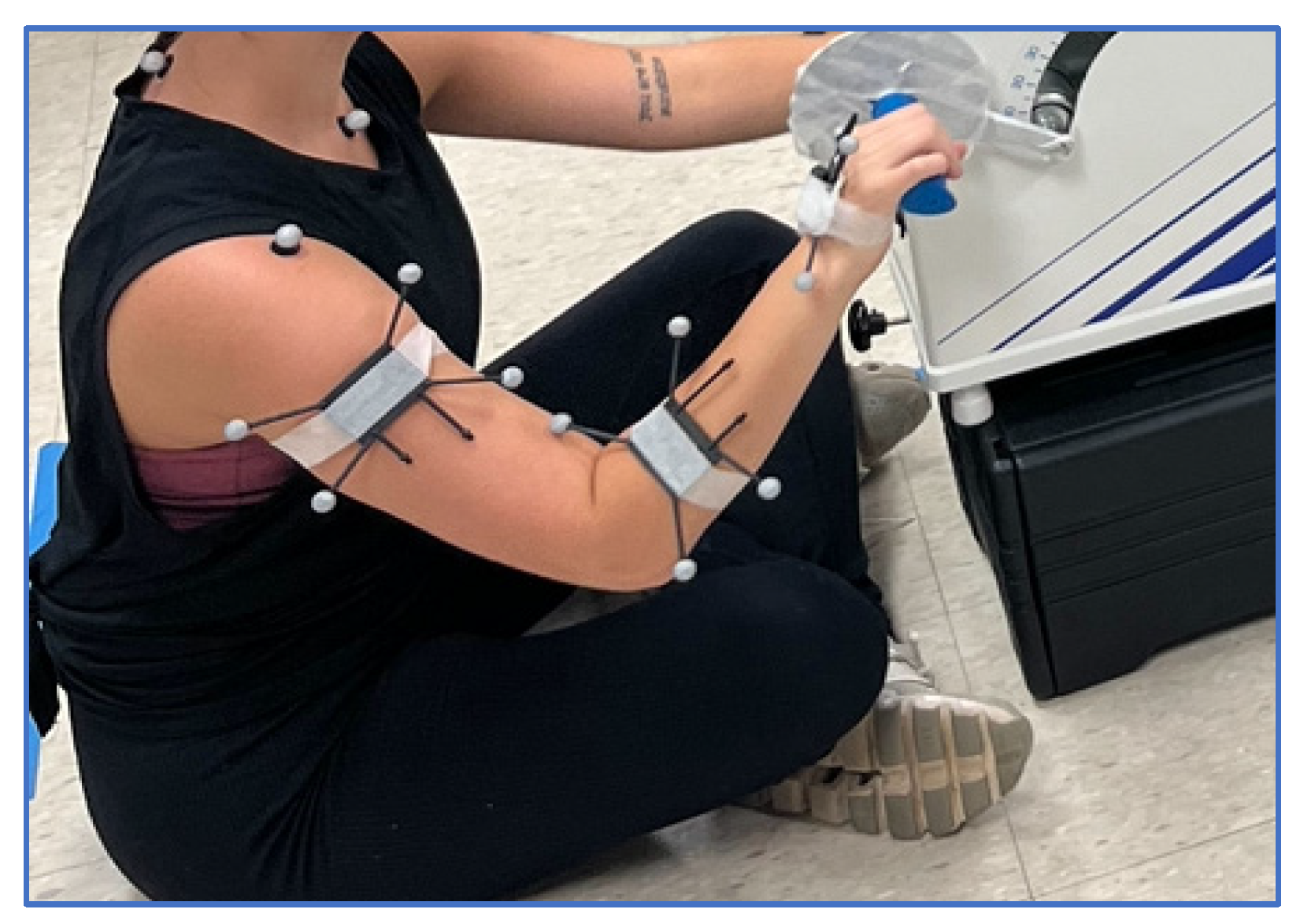
2.4. Experimental Protocol
2.5. Data Processing
2.6. Statistical Analysis
3. Results
3.1. Reliability
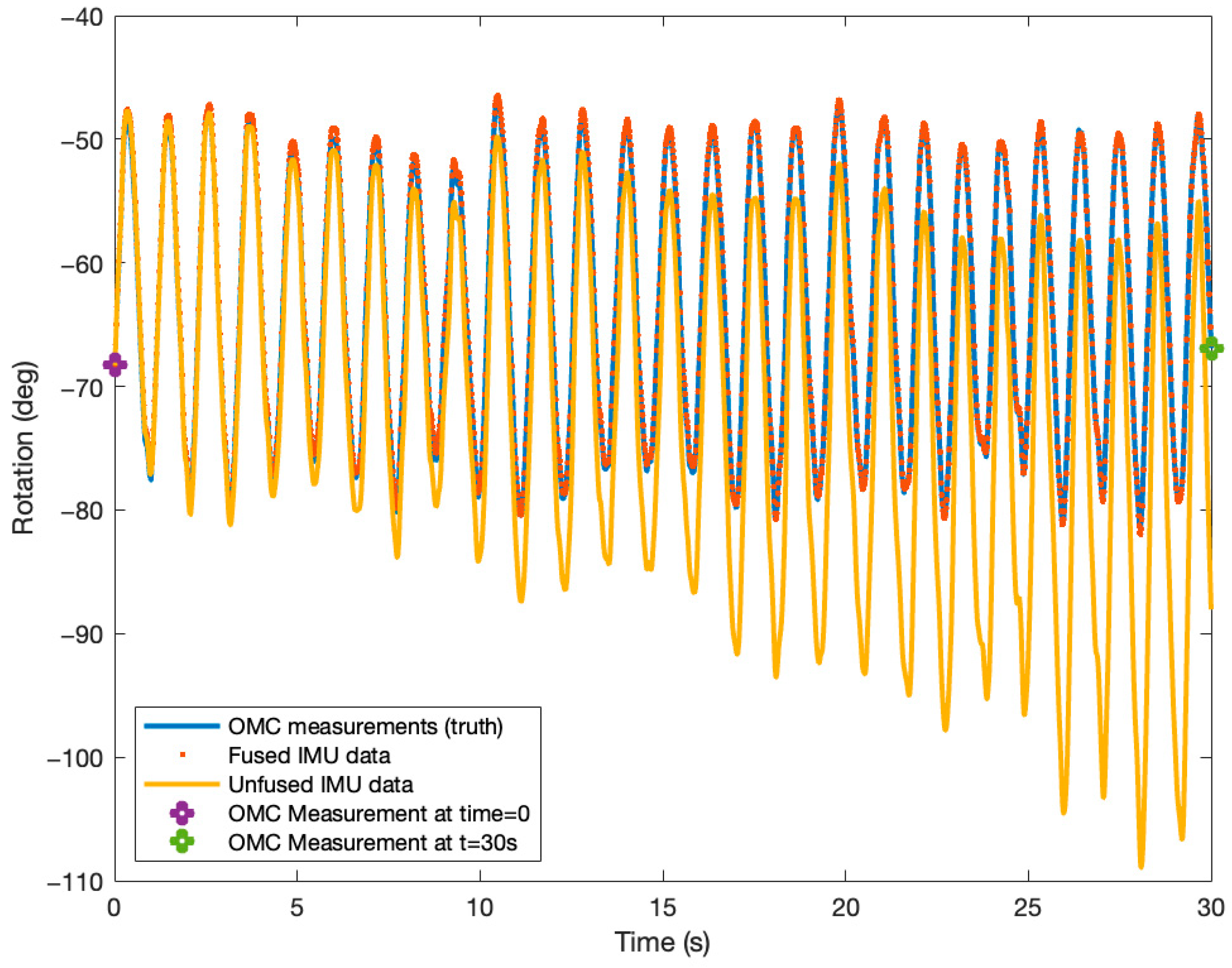
3.2. Total Error
4. Discussion
4.1. Reliability of the Algorithm
4.2. OMC-IMC Errors
4.3. Limitations
4.4. Implications
5. Conclusions
Author Contributions
Funding
Institutional Review Board Statement
Informed Consent Statement
Data Availability Statement
Acknowledgments
Conflicts of Interest
Abbreviations
| OMC | Optical Motion Capture |
| IMC | Inertial Motion Capture |
| IMU | Inertial Measurement Unit |
| ROM | Range of Motion |
| SPSS | Statistical Package for Social Sciences |
| CI | Confidence Interval |
| ANOVA | Analysis of Variance |
| ICC | Intraclass Correlation Coefficients |
| SD | Standard Deviation |
| ESKF | Error-state Kalman Filter |
| UKF | Unscented Kalman Filter |
| RSME | Root-Mean-Square Error |
References
- Cuesta-Vargas, A.I.; Galán-Mercant, A.; Williams, J.M. The use of inertial sensors system for human motion analysis. Phys. Ther. Rev. 2010, 15, 462–473. [Google Scholar] [CrossRef] [PubMed]
- Cappozzo, A.; Della Croce, U.; Leardini, A.; Chiari, L. Human movement analysis using stereophotogrammetry: Part 1: Theoretical background. Gait Posture 2005, 21, 186–196. [Google Scholar] [CrossRef] [PubMed]
- Eichelberger, P.; Ferraro, M.; Minder, U.; Denton, T.; Blasimann, A.; Krause, F.; Baur, H. Analysis of accuracy in optical motion capture—A protocol for laboratory setup evaluation. J. Biomech. 2016, 49, 10. [Google Scholar] [CrossRef]
- Aurand, A.M.; Dufour, J.S.; Marras, W.S. Accuracy map of an optical motion capture system with 42 or 21 cameras in a large measurement volume. J. Biomech. 2017, 58, 237–240. [Google Scholar] [CrossRef]
- Merriaux, P.; Dupuis, Y.; Boutteau, R.; Vasseur, P.; Savatier, X. A study of vicon system positioning performance. Sensors 2017, 17, 1591. [Google Scholar] [CrossRef]
- Yang, P.-F.; Sanno, M.; Brüggemann, G.-P.; Rittweger, J. Evaluation of the performance of a motion capture system for small displacement recording and a discussion for its application potential in bone deformation in vivo measurements. Proc. Inst. Mech. Eng. 2012, 226, 838–847. [Google Scholar] [CrossRef]
- Camargo, J.; Ramanathan, A.; Csomay-Shanklin, N.; Young, A. Automated gap-filling for marker-based biomechanical motion capture data. Comput. Methods Biomech. Biomed. Engin. 2020, 23, 1180–1189. [Google Scholar] [CrossRef]
- Gomes, D.; Guimarães, V.; Silva, J. A Fully-Automatic Gap Filling Approach for Motion Capture Trajectories. Appl. Sci. 2021, 11, 9847. [Google Scholar] [CrossRef]
- Tits, M.; Tilmanne, J.; Dutoit, T. Robust and automatic motion-capture data recovery using soft skeleton constraints and model averaging. PLoS ONE 2018, 13, e0199744. [Google Scholar] [CrossRef]
- Liu, G.; McMillan, L. Estimation of missing markers in human motion capture. Vis. Comput 2006, 22, 721–728. [Google Scholar] [CrossRef]
- Smolka, J.; Lukasik, E. The rigid body gap filling algorithm. In Proceedings of the 2016 9th International Conference on Human System Interactions (HSI), Portsmouth, UK, 6–8 July 2016; pp. 337–343. [Google Scholar] [CrossRef]
- Roetenberg, D.; Luinge, H.; Slycke, P. Xsens MVN: Full 6DOF Human Motion Tracking Using Miniature Inertial Sensors. Xsens Technol. 2013, 1, 1–7. [Google Scholar]
- Brodie, M.A.; Walmsley, A.; Page, W. Dynamic accuracy of inertial measurement units during simple pendulum motion. Comput. Methods Biomech. Biomed. Engin. 2008, 11, 235–242. [Google Scholar] [CrossRef]
- Chen, H.; Schall, M.C.; Fethke, N.B. Measuring upper arm elevation using an inertial measurement unit: An exploration of sensor fusion algorithms and gyroscope models. Appl. Ergon. 2020, 89, 103187. [Google Scholar] [CrossRef] [PubMed]
- Pellatt, L.; Dewar, A.; Philippides, A.; Roggen, D. Mapping vicon motion tracking to 6-axis IMU data for wearable activity recognition. In Activity and Behavior Computing; Ahad, M.A.R., Inoue, S., Roggen, D., Fujinami, K., Eds.; Springer: Singapore, 2021; pp. 3–20. [Google Scholar] [CrossRef]
- Gonzalez, R.; Dabove, P. Performance assessment of an ultra low-cost inertial measurement unit for ground vehicle navigation. Sensors 2019, 19, 3865. [Google Scholar] [CrossRef] [PubMed]
- Chen, H.; Schall, M.C.; Fethke, N. Effects of Movement Speed and Magnetic Disturbance on the Accuracy of Inertial Measurement Units. Proc. Hum. Factors Ergon. Soc. Annu. Meet. 2017, 61, 1046–1050. [Google Scholar] [CrossRef] [PubMed]
- Suvorkin, V.; Garcia-Fernandez, M.; González-Casado, G.; Li, M.; Rovira-Garcia, A. Assessment of Noise of MEMS IMU Sensors of Different Grades for GNSS/IMU Navigation. Sensors 2024, 24, 1953. [Google Scholar] [CrossRef] [PubMed]
- Lebel, K.; Boissy, P.; Hamel, M.; Duval, C. Inertial measures of motion for clinical biomechanics: Comparative assessment of accuracy under controlled conditions-effect of velocity. PLoS ONE 2013, 8, e79945. [Google Scholar] [CrossRef]
- Plamondon, A.; Delisle, A.; Larue, C.; Brouillette, D.; McFadden, D.; Desjardins, P.; Larivière, C. Evaluation of a hybrid system for three-dimensional measurement of trunk posture in motion. Appl. Ergon. 2007, 38, 697–712. [Google Scholar] [CrossRef]
- Yang, Z.; Yan, S.; van Beijnum, B.-J.F.; Li, B.; Veltink, P.H. Improvement of optical tracking-based orientation estimation by fusing gyroscope information. IEEE Trans. Instrum. Meas. 2021, 70, 9508913. [Google Scholar] [CrossRef]
- Enayati, N.; Momi, E.D.; Ferrigno, G. A quaternion-based unscented kalman filter for robust optical/inertial motion tracking in computer-assisted surgery. IEEE Trans. Instrum. Meas. 2015, 64, 2291–2301. [Google Scholar] [CrossRef]
- Hicks, H.N.; Harper, S.A.; Chen, H. Sensor Fusion for enhancing motion capture: Integrating optical and inertial motion capture systems. In Proceedings of the Aspire—69th Human Factors and Ergonomics Society Annual Meeting, Chicago, IL, USA, 13–17 October 2025. Accepted. [Google Scholar]
- Kok, M.; Hol, J.D.; Schön, T.B. Using Inertial Sensors for Position and Orientation Estimation. Found. Trends Signal Process. 2017, 11, 1–153. [Google Scholar] [CrossRef]
- Available online: https://github.com/uah-crablab/imu-omc-fusion (accessed on 6 June 2025).
- Wahba, G. A least squares estimate of satellite attitude. SIAM Rev. 1965, 7, 409. [Google Scholar] [CrossRef]
- Faber, G.S.; Kingma, I.; Chang, C.C.; Dennerlein, J.T.; van Dieën, J.H. Validation of a wearable system for 3D ambulatory L5/S1 moment assessment during manual lifting using instrumented shoes and an inertial sensor suit. J. Biomech. 2020, 102, 109671. [Google Scholar] [CrossRef]
- Koo, T.K.; Li, M.Y. A Guideline of Selecting and Reporting Intraclass Correlation Coefficients for Reliability Research. J. Chiropr. Med. 2016, 15, 155–163. [Google Scholar] [CrossRef]
- Liljequist, D.; Elfving, B.; Roaldsen, K.S. Intraclass correlation-A discussion and demonstration of basic features. PLoS ONE 2019, 14, e0219854. [Google Scholar] [CrossRef] [PubMed]
- Chen, H.; Schall, M.C.; Martin, S.M.; Fethke, N.B. Drift-Free joint angle calculation using inertial measurement units without magnetometers: An exploration of sensor fusion methods for the elbow and wrist. Sensors 2023, 23, 7053. [Google Scholar] [CrossRef]
- Godwin, A.; Agnew, M.; Stevenson, J. Accuracy of inertial motion sensors in static, quasistatic, and complex dynamic motion. J. Biomech. Eng. 2009, 131, n114501. [Google Scholar] [CrossRef]
- Robert-Lachaine, X.; Mecheri, H.; Larue, C.; Plamondon, A. Effect of local magnetic field disturbances on inertial measurement units accuracy. Appl. Ergon. 2017, 63, 123–132. [Google Scholar] [CrossRef]
- Chen, H.; Schall, M.C.; Fethke, N.B. Gyroscope vector magnitude: A proposed method for measuring angular velocities. Appl. Ergon. 2023, 109, 103981. [Google Scholar] [CrossRef]
- Bachmann, E.R.; Yun, X.; Peterson, C.W. An investigation of the effects of magnetic variations on inertial/magnetic orientation sensors. In Proceedings of the IEEE International Conference on Robotics and Automation, ICRA, New Orleans, LA, USA, 26 April–1 May 2004; Volume 2, pp. 1115–1122. [Google Scholar] [CrossRef]

| Placement | Time Interval | ICC | Confidence Interval |
|---|---|---|---|
| Hand Z | 5 | 0.998 | (0.993, 0.999) |
| Hand Y | 5 | 1.000 | (0.999, 1.000) |
| Hand X | 5 | 0.996 | (0.987, 0.999) |
| Forearm Z | 5 | 0.998 | (0.994, 0.999) |
| Forearm Y | 5 | 0.999 | (0.998, 1.000) |
| Forearm X | 5 | 0.995 | (0.983, 0.999) |
| Upper Arm Z | 5 | 0.999 | (0.997, 1.000) |
| Upper Arm Y | 5 | 0.996 | (0.987, 0.999) |
| Upper Arm X | 5 | 0.997 | (0.990, 0.999) |
| Error | 1-min | 2-min | 5-min |
|---|---|---|---|
| X-Axis | 1.1 (0.7) | 1.4 (0.9) | 1.7 (1.0) |
| Y-Axis | 0.3 (0.1) | 0.3 (0.2) | 0.4 (0.2) |
| Z-Axis | 0.3 (0.2) | 0.4 (0.2) | 0.6 (0.4) |
| Total | 1.2 (0.7) | 1.5 (0.9) | 1.8 (1.0) |
| Error | 1-min | 2-min | 5-min |
|---|---|---|---|
| X-Axis | 0.8 (0.2) | 0.8 (0.3) | 0.8 (0.3) |
| Y-Axis | 0.4 (0.3) | 0.5 (0.3) | 0.7 (0.5) |
| Z-Axis | 0.4 (0.2) | 0.4 (0.2) | 0.6 (0.3) |
| Total | 1.0 (0.3) | 1.0 (0.3) | 1.3 (0.4) |
| Error | 1-min | 2-min | 5-min |
|---|---|---|---|
| X-Axis | 0.5 (0.2) | 0.9 (0.3) | 0.7 (0.4) |
| Y-Axis | 0.4 (02) | 0.5 (0.2) | 0.4 (0.2) |
| Z-Axis | 0.6 (0.3) | 0.6 (0.3) | 0.7 (0.4) |
| Total | 0.9 (0.3) | 1.0 (0.3) | 1.1 (0.5) |
Disclaimer/Publisher’s Note: The statements, opinions and data contained in all publications are solely those of the individual author(s) and contributor(s) and not of MDPI and/or the editor(s). MDPI and/or the editor(s) disclaim responsibility for any injury to people or property resulting from any ideas, methods, instructions or products referred to in the content. |
© 2025 by the authors. Licensee MDPI, Basel, Switzerland. This article is an open access article distributed under the terms and conditions of the Creative Commons Attribution (CC BY) license (https://creativecommons.org/licenses/by/4.0/).
Share and Cite
Hicks, H.N.; Chen, H.; Harper, S.A. Sensor Fusion for Enhancing Motion Capture: Integrating Optical and Inertial Motion Capture Systems. Sensors 2025, 25, 4680. https://doi.org/10.3390/s25154680
Hicks HN, Chen H, Harper SA. Sensor Fusion for Enhancing Motion Capture: Integrating Optical and Inertial Motion Capture Systems. Sensors. 2025; 25(15):4680. https://doi.org/10.3390/s25154680
Chicago/Turabian StyleHicks, Hailey N., Howard Chen, and Sara A. Harper. 2025. "Sensor Fusion for Enhancing Motion Capture: Integrating Optical and Inertial Motion Capture Systems" Sensors 25, no. 15: 4680. https://doi.org/10.3390/s25154680
APA StyleHicks, H. N., Chen, H., & Harper, S. A. (2025). Sensor Fusion for Enhancing Motion Capture: Integrating Optical and Inertial Motion Capture Systems. Sensors, 25(15), 4680. https://doi.org/10.3390/s25154680