1. Introduction
As a core industrial technology, welding is extensively applied in advanced manufacturing sectors such as aerospace, shipbuilding, rail transit, and machinery, playing a vital role in national economic development and technological advancement [
1]. Achieving stable and high-quality welds—characterized by defect-free surfaces, consistent geometry, and reliable mechanical properties—requires optimal process design, precise parameter control, skilled operation, and robust quality assurance. However, due to the complex, dynamic, and nonlinear nature of the welding process, various defects are often unavoidable, and detecting them in real time remains challenging [
2]. Experienced welders manually detect defects by observing the molten pool. However, prolonged observation causes fatigue, slower responses, and lower quality, while welding fumes also pose health risks. These challenges have driven global research efforts toward automated molten pool vision systems that can continuously monitor welding quality and detect defects in real time, thereby improving efficiency and safety.
The current research field of welding defect recognition and monitoring in the welding process is divided into two main categories: the first method focuses on welding defect detection using a single-frame molten pool image; the second method realizes welding defect recognition by analyzing the spatiotemporal dynamic information embedded in the molten pool image sequence.
Welding defect detection based on single-frame molten pool images typically relies on analyzing static frames captured at a single time point. Traditional machine learning methods employ algorithms such as decision trees, support vector machines (SVMs), and random forests (RFs) to simulate expert decision-making [
3,
4,
5,
6,
7]. These methods are interpretable but depend on expert knowledge and precise camera–robot alignment. End-to-end CNNs eliminate manual feature design and have achieved improved accuracy and efficiency through architectural enhancements [
2,
8,
9,
10,
11,
12,
13], while hybrid approaches that fuse deep and handcrafted features further bolster interpretability and robustness [
14,
15]. However, visual similarities across welding conditions continue to limit the reliability of single-frame analysis in real-world scenarios. Compared to single-frame methods, multi-frame methods utilize time-series molten pool images, providing richer dynamic information for robust weld quality monitoring. Some scholars have utilized typical timing processing methods to establish welding defect detection models; for example, Lu et al. [
1] used an LSTM-based prediction–classification framework to model temporal morphology changes up to ten frames ahead, while Chen et al. [
16] fused CNN–LSTM visual features with arc signal time–frequency features for improved GTAW state recognition. Liu et al. [
17] proposed a lightweight 3DCNN (3DSMDA-Net) that decomposes 3D convolutions and incorporates multidimensional attention to reduce computation without sacrificing accuracy. Despite these advances, real-time deployment remains challenging, prompting frame-fusion strategies such as that by Jiao et al. [
18], who combined adjacent frames into a single image for efficient 2D-CNN processing.
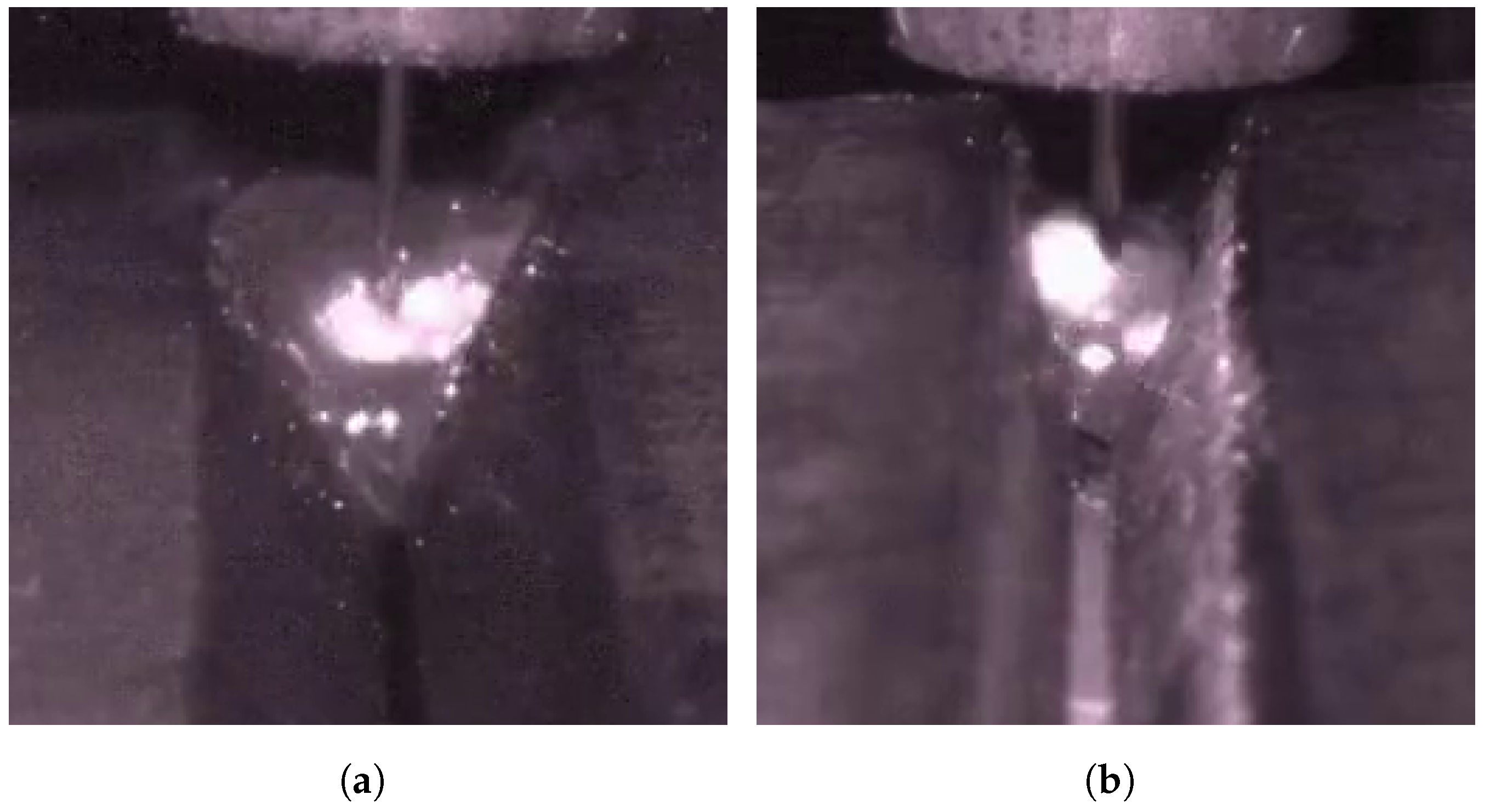
In addition, in the actual welding process, welding defect detection using molten pool images still faces many challenges. As shown in
Figure 1a,b, the interclass similarity problem poses a major difficulty in recognizing welding defects. Due to the extremely complex heat transfer and molten metal flow processes in the weld pool, the normal pool and the defective (e.g., porosity) pool are highly similar regarding surface spot distribution, texture characteristics, and overall appearance. This similarity makes it very easy for the traditional single-frame image analysis method to misjudge the welding state, thereby reducing the accuracy and reliability of the identification. Meanwhile, as shown in
Figure 1c,d, the problem of intraclass variability also hinders the stability of molten pool image analysis. Even under the same welding condition (e.g., a normal molten pool), the molten pool images may be affected by the interference of spatter particles, changes in the intensity of the molten pool flow, and small differences in the shooting angle and illumination conditions, resulting in large differences in the morphology, texture, and brightness distribution of the molten pool. This significant intraclass variability increases the difficulty of the model in accurately identifying the steady state, which in turn reduces the stability of the actual detection. To address these issues, Hong et al. [
8] address these challenges with LDI-MSARL-net, which employs multi-granularity spatiotemporal attention, a dual-branch global–local fusion, and dynamic enhancement to improve feature discrimination. Despite such progress, efficiently and reliably overcoming both interclass similarity and intraclass variability in real-world molten pool images remains an open challenge.
Previous studies have shown the potential value of applying spatiotemporal feature information to weld defect monitoring. However, some existing detection methods still have some problems: (1) The “black box” nature of deep learning makes it difficult to trace the decision logic of the model, while welding defect detection needs to meet the strong interpretability requirements of industrial scenarios (e.g., defect attribution analysis). Techniques like CAM or Grad-CAM [
19] highlight high-level activations but cannot link them to physical molten pool characteristics (e.g., temperature or geometry). Fusing handcrafted descriptors—such as LBP for surface roughness [
20] and HOG for contour aberrations—with CNN features (e.g., ResNet-50 activation maps [
21]) via multimodal alignment preserves interpretability while reducing overfitting. (2) The problem of molten pool image interference (e.g., the reflected spot of the laser on the spatter is misclassified as a stomatal defect) in a complex welding scene is prominent. Some attentional mechanisms can overcome the interclass similarity problem of defects on a spatial scale, but in contrast, learning key unobstructed frames in time-series images may bring better results for recognizing such images. Considering both the interclass similarity of defects as well as the intraclass diversity problem, we use a multi-granular spatiotemporal attention mechanism for molten pool time-series images.
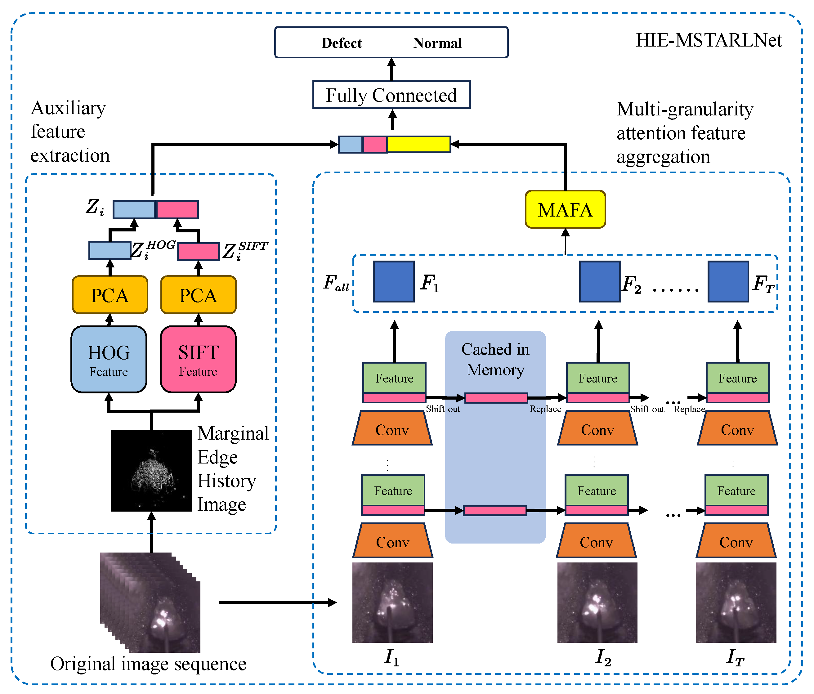
Inspired by previous research, we propose a multi-granularity spatiotemporal attention learning network (HIE-MSTARLNet). This network integrates temporal deep learning features with long-term dynamic information to address these challenges. The main contributions of this paper are summarized as follows.
We propose an innovative welding defect detection method that integrates the selection of key interference-free frames into a multi-granularity spatiotemporal attention mechanism, thereby overcoming the limitations of existing approaches in extracting critical information from highly redundant, interference-prone molten pool time-series images;
Simultaneously aggregating long-term dynamic information of fusion pool time-series images and multi-level semantic features in the spatial dimension of time-series deep learning features is achieved, effectively solving the problem of insufficient interpretability and the problem of interclass similarity and intraclass diversity of deep learning;
Based on the collected data on actual weld porosity defects, the effectiveness of the proposed method is verified through careful evaluation experiments, comparison experiments with typical methods, and visualization analysis.
3. Experimental Design
3.1. Dataset
High-quality datasets are fundamental for algorithm validation. In this study, Gas Metal Arc Welding (GMAW) was employed with two types of welding wire (solid wire and flux-cored wire), and 980 high-strength steel was used as the base material. Welds with varying root gaps and groove angles were prepared, and a molten pool vision system was used to capture videos of both normal and porosity-defect molten pools on 30 welding plates in flat and vertical welding positions [
31]. The normal and porosity-defect samples from four of these plates were selected to form the test set. Videos were recorded at a pixel resolution of 640 × 512 and 30 fps, then segmented into 1-s clips with one sample taken every 4 s. Eight frames were evenly extracted from each clip, yielding approximately 600 samples per class—substantially more than classic datasets such as HMDB51 (average of about 101 per category) [
32] and UCF101 (average of about 137 per category) [
33].
In real welding scenarios, molten pool images include regions of the weld seam, base metal, welding torch, and the molten pool itself; however, the molten pool—the core region for defect detection—occupies only a small portion of each image. High-resolution images contain redundant background information, increasing the computational load and hindering effective feature extraction from critical regions. Therefore, for each sample’s eight frames, the molten pool region was first segmented. Based on these segmentation results, the molten pool region was cropped from the original image with a 1:1 aspect ratio and then resized to 224 × 224 pixels without altering the pool’s original aspect ratio—this served as the input for deep learning models. This preprocessing scheme preserves image detail while improving processing speed by a factor of four without compromising accuracy. The resulting dataset, named WELDPOOL, was split into 60% training, 10% validation, and 30% test sets.
3.2. Test Environment
In our experiments, we used a desktop computer with a GeForce RTX 3060 GPU and a 12th-generation Intel(R) Core(TM) i9-12900H CPU running Windows 11. The WELDPOOL dataset was utilized, and the dataset was divided into the training, validation, and test sets in the ratio of 6:1:3. The experimental hyperparameters were set: the initial learning rate was 0.001; the weight decay was 0.0001; the momentum was 0.9; stochastic gradient descent was used to update the parameters; cosine annealing was used to adjust the learning rate; the number of training rounds was still set to 50; the batch size of each training iteration was set to 4, and the model was saved every three rounds with the best and final models. This ensures training stability while maximizing model convergence efficiency.
3.3. Performance Metrics
To objectively evaluate the effectiveness of the proposed model in identifying porosity defects, this study assesses the model from both performance and real-time capability perspectives. We use accuracy (Top-1 and Top-5), recall, and the F1-score as key metrics for performance evaluation. We also consider the number of parameters and computational complexity as evaluation criteria. Additionally, we include inference latency as a real-time evaluation metric.
3.4. Experiments
The experiments were conducted in the environment specified in
Section 3.2. Firstly, we performed a training parameter analysis, testing the impact of data augmentation, fused image types, frame counts, and granularity levels on experimental performance to determine the final experimental parameters. Next, ablation experiments were carried out; specifically, experiments were conducted by separately excluding TSM, MAFA, and LDSSI auxiliary enhancement from the HIE-MSTARLNet model to illustrate the necessity and effectiveness of these technical modules. We then compared the specific performance of the model under different types of fused images and also compared it with several typical baseline welding defect detection models, demonstrating the superiority of the proposed approach. Additionally, confusion matrices of different methods were analyzed to further illustrate their effectiveness. We also tested normal molten pool samples under different conditions to analyze factors affecting performance. Finally, heatmap visualization tests were performed on molten pools from different welding state categories to analyze regions considered important by the model for defect identification.
4. Experimental Results
To speed up the training time, the MEHI as well as the frequency domain fusion images of the existing dataset are first computed here, and the PCA model that reduces the HOG and SIFT features to 100 dimensions is trained separately. In training, the multiple data loading form is used to directly input the original fusion pool image sequence and the generated MEHI or frequency domain fusion image, which eliminates the step of frequently calculating the MEHI and frequency domain fusion image; in the inference stage, the single data loading form is used to join the process of MEHI generation or frequency domain fusion image generation, which facilitates the calculation of the time spent on inference for each sample. And to further validate the interference resistance of the proposed model, data enhancement is carried out by adding random noise, flipping, rotating, and lighting changes to simulate as much as possible the various problems that may be encountered in a real welding scene.
4.1. Ablation Study
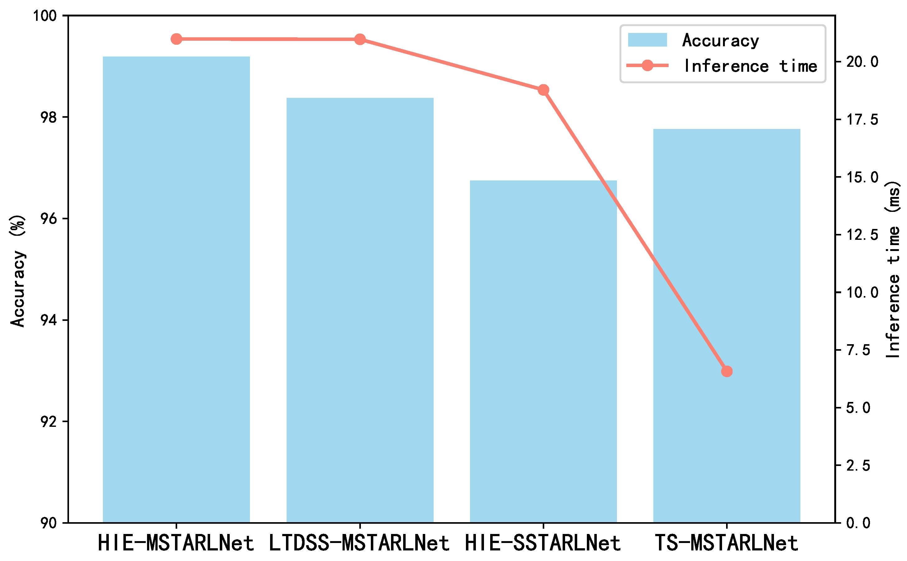
The core of the HIE-MSTARLNet model lies in the TSM, Multi-granularity Attention Feature Aggregation (MAFA), and long-term dynamic spatial structure information (LDSSI) aids. To this end, an ablation study was conducted to illustrate the necessity and effectiveness of these technical modules on the model. Specifically, the TSM, MAFA, and LDSSI-assisted augmentation from the HIE-MSTARLNet model, the long-term dynamic spatial structure information-augmented multi-granularity spatialtemporal representation learning network (LTDSS-MSTARLNet), the long-term dynamic spatial structure information-augmented single-granularity spatialtemporal representation learning network (HIE (HIE-SSTARLNet), the single-grained spatiotemporal representation learning network enhanced with long-term dynamic spatial structure information and time-shift information (SSTARLNet), and the time-shift information-enhanced multi-gradient spatiotemporal representation learning network (TS-MSTARLNet) were excluded. Then the performance of the three models is evaluated by accuracy and inference time, and the comparison results are shown in
Figure 7.
From the figure, it can be seen that all three auxiliary enhancement tools, TSM, MAFA, and LDSSI, contribute to the performance of the model, and among them, TSM and MAFA contribute to a greater extent than the LDSSI auxiliary enhancement tool (i.e., TS-MSTARLNet has higher accuracy than the LTDSS-MSTARLNet model and the HIE-SSTARLNet model on the self-constructed dataset). The LTDSS-MSTARLNet model has higher accuracy than the HIE-SSTARLNet model on the self-constructed dataset, where MAFA contributes to a greater extent than the TSM (i.e., the LTDSS-MSTARLNet model has higher accuracy than the HIE-SSTARLNet model). However, both the MAFA module and the LDSSI-assisted enhancement tool significantly increase the inference time, whereas the TSM, being a plug-and-play module, adds little to no inference time. Among them, the MAFA module increases the inference time related to the number of its granularity levels, so it is important to minimize the granularity levels to reduce the inference time while satisfying high accuracy.
Overall, the ablation experiments of HIE-MSTARLNet validate the differentiated contributions of the three modules, TSM, MAFA, and LDSSI, to the model’s performance, providing a quantitative basis for the modular design of industrial vision models.
4.2. Comparative Result Analysis
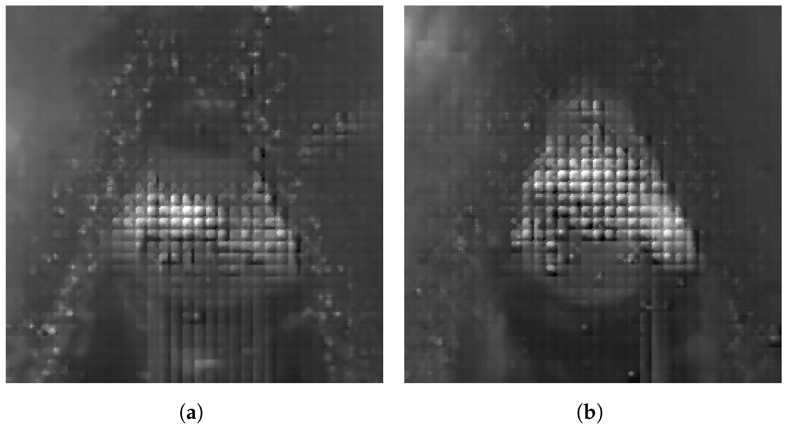
To further illustrate the actual metrics performance of the HIE-MSTARLNet model using MEHIs and the HIE-MSTARLNet model using the frequency-domain fusion image (FDFI), the accuracy, precision, recall, F1 score, and inference time of the two models using different inputs are compared, as shown in
Table 1,
Although inference times are comparable between the two methods, the HIE-MSTARLNet model based on the MEHI significantly outperforms the model using the FDFI in terms of accuracy and other key evaluation metrics. This advantage primarily stems from the superior feature representation provided by the MEHI approach. Specifically, the MEHI effectively integrates spatiotemporal dynamic information of the welding process by preserving historical edge details of the molten pool region across consecutive frames. This edge-history information not only captures subtle temporal variations in molten pool boundaries but also emphasizes minor structural differences in defect regions, facilitating more accurate defect identification. Additionally, the MEHI performs fusion directly in the spatial domain, thereby avoiding potential information loss and noise interference associated with frequency-domain transformations, enabling precise retention of essential local features at the original spatial resolutions. In contrast, the probable reason for the lower performance of the FDFI-based model is that additional noise may be introduced during the frequency-domain fusion process, which interferes with the model’s learning of effective features and weakens the high-resolution features of key local structures in the spatial domain due to the global frequency-domain transform, such as the formation of mosaic regions in the molten pool image, leading to a degradation of the model’s performance.
To demonstrate the superiority of the constructed weld defect detection model, the model was compared against several typical baselines of weld defect detection models, including a comparison of one class of models using static input data (i.e., image-based methods) and three classes of models using dynamic input data (i.e., RNN-based methods, 3-DCNN-based methods, and image fusion (IF) methods). For the three types of models using dynamic input data, the TSM, Multi-granularity Feature Aggregation (MGFA), and the attention module are sequentially inserted into the appropriate positions in the existing models to compare the performance of the model with the whole process of temporal feature extraction and the model with only temporal feature extraction at the end, as well as the performance of the model with the full process of temporal feature extraction and the performance of the model with only temporal feature extraction at the end. Specifically, all three types of models using dynamic data inputs use TSM; for the attention module, spatial and channel attention are used for the RNN-based and image fusion-based models, and spatial, channel, and temporal attentions are used for the 3-DCNN-based model. For a fair comparison, all models use MobileNetV2 as the backbone network and use consistent hyperparameter settings during the training phase. In particular, the optimal parameter values for model-specific hyperparameters (e.g., the time step and hidden cell number for the RNN-based approach and the input frame sequence length for the 3-DCNN-based and IF-based approaches) were filtered by a grid search and five-fold cross-validation, combining the typical values tested during previous training sessions and the actual test results in this experiment.
Table 2 details the final comparison results of the four methods on the test dataset.
To avoid model chance, the values in the experiments are averaged over five cross-experiment runs as an evaluation metric. In terms of classification performance, these methods considering time-series information outperform image-based methods; feature-level fusion in time-series methods outperforms pixel-level fusion, and models fusing temporal information throughout the process also usually outperform methods fusing temporal information only at the end. Specifically, in these model comparisons, the proposed HIE-MSTARLNet model significantly outperforms other existing baseline methods by achieving 99.187%, 99.210%, 99.187%, and 99.190% in terms of accuracy (Acc), precision (Pre), recall (Rec), and F1 values, respectively. And, in terms of the inference time, methods that introduce temporal information generally take longer than single-image static methods (especially 3D-CNN-based methods), but HIE-MSTARLNet dramatically reduces the inference time while improving classification performance. And HIE-MSTARLNet has higher accuracy than MFVNet, but the inference time is a bit longer than MFVNet; the main reason comes from the generation time of MEHI, but in the actual deployment process, which is different from the MEHI inference experiments that generate the whole sample each time, the edge information of the first seven frames of the image can be cached at a specific time while actual receiving melting pool camera images, only the edge information of the current frame needs to be calculated, and weighted fusion needs to be performed; therefore, the inference time of the HIE-MSTARLNet model in practical applications can be greatly reduced.
To further analyze the model’s classification ability for different welding states, we select the optimal model from each of the five classes of methods (static image-based methods, RNN-based methods, 3D-CNN-based methods, pixel-level methods based on image fusion, and feature-level methods based on image fusion) and draw a normalized confusion matrix based on the classification results of the test set, as shown in
Figure 8.
Each method has a small number of normal samples that are misclassified as pore defects, but the HIE-MSTARLNet model misclassifies fewer samples and is accurate in identifying pore defects, with only a small number of misclassified samples among the correct samples.
Therefore, to further analyze the sensitivity of the model in each sample, samples of normal molten pools with different conditions were tested. The results are shown in
Table 3.
It can be observed that the HIE-MSTARLNet model has an accuracy of more than 99.7% in recognizing changes in the shape and size of the molten pool, and the accuracy in the splash interference scenario also reaches 98.374%. This indicates that the HIE-MSTARLNet model has improved anti-interference ability compared to the MFVNet model and can accurately recognize normal samples.
4.3. Visual Analysis
To further illustrate the interpretability of the proposed HIE-MSTARLNet model and to intuitively highlight its decision-making process in weld defect identification, we utilized class activation mapping (CAM) visualization. Specifically, molten pool images from four representative cases (CAM1–CAM4), covering both normal and porosity-defect scenarios, were selected for visualization, as shown in
Figure 9. The first row corresponds to normal molten pools, and the second row corresponds to pools exhibiting porosity defects. The CAM results indicate that the model primarily focuses its attention on the central region of the molten pool surface, specifically the molten metal region below the welding wire. This central area exhibits notable variations in texture patterns and light spot distributions between normal and defective states, as opposed to solely relying on the outer contours of the molten pool, which has traditionally been the primary focus of previous studies. Notably, our visualizations also indicate that spatter around the molten pool is one potential interfering factor that might lead to misclassification. In practical industrial applications, these visual insights can effectively guide weld quality control by allowing operators and engineers to observe and understand critical discriminative features associated with defects directly. For example, noticing subtle differences in the highlighted central region may facilitate timely parameter adjustments or welding wire changes before significant defects occur. Thus, these CAM visualizations not only enhance the interpretability of the proposed model from a theoretical perspective but also offer actionable insights for industrial deployment, thereby bridging the gap between theoretical advances and real-world welding quality management.
4.4. Training and Parameter Analysis
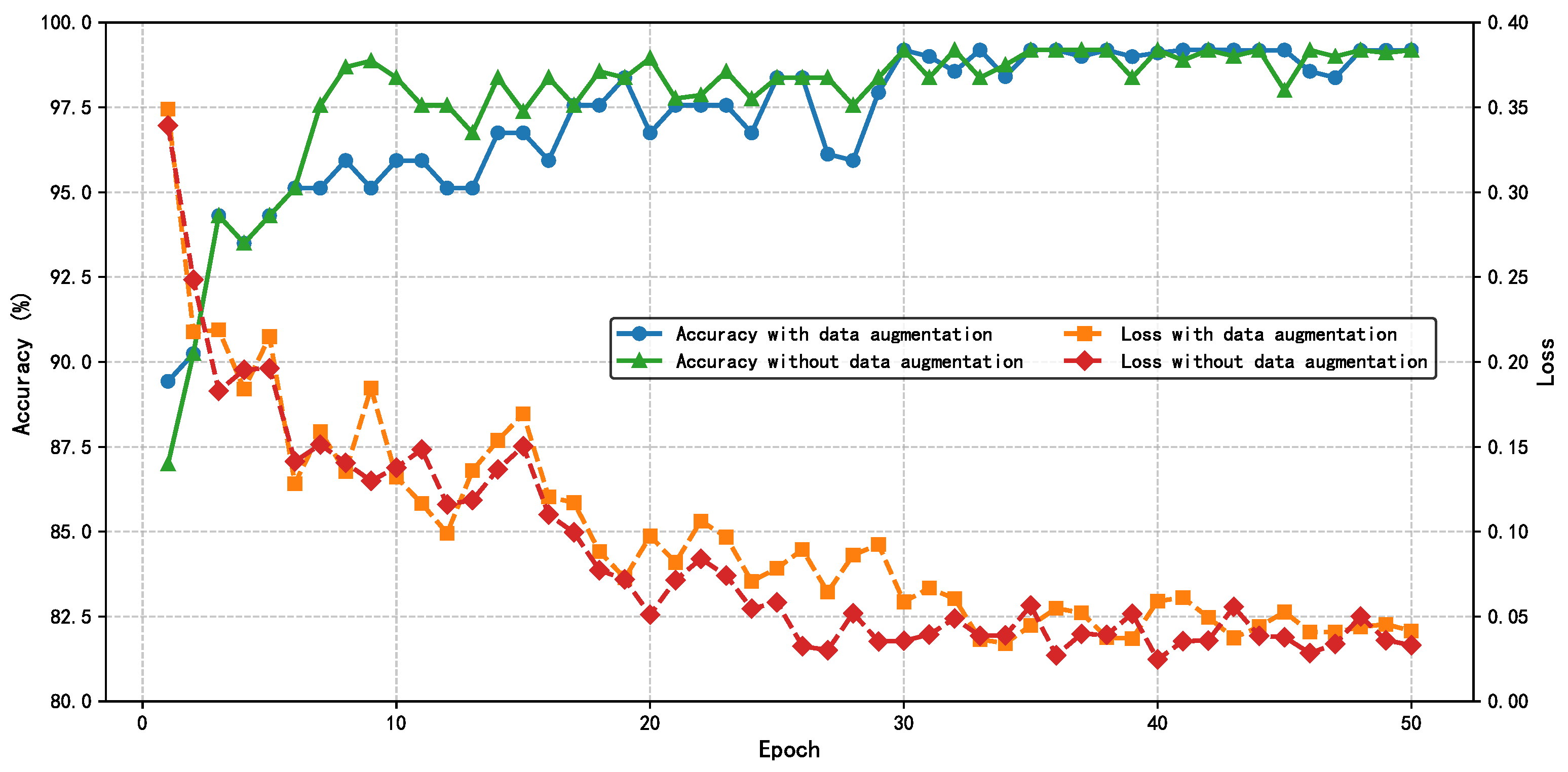
The HIE-MSTARLNet model is first trained using MEHI images and raw sequence images, and the process is shown in
Figure 10. It can be seen that the model trained based on the data after data augmentation exhibits more stable accuracy after convergence, although it converges more slowly than the model trained based on the original data. Moreover, the overall stability of the model improves significantly after data augmentation, and its performance stabilizes after about 35 epochs. To prevent overfitting, an early stopping strategy is used, where the number of training rounds is set to 10 rounds, and the model stops training at 42 rounds, so the model with 42 training rounds is used as the final model of the HIE-MSTARLNet model using MEHIs for the subsequent study.
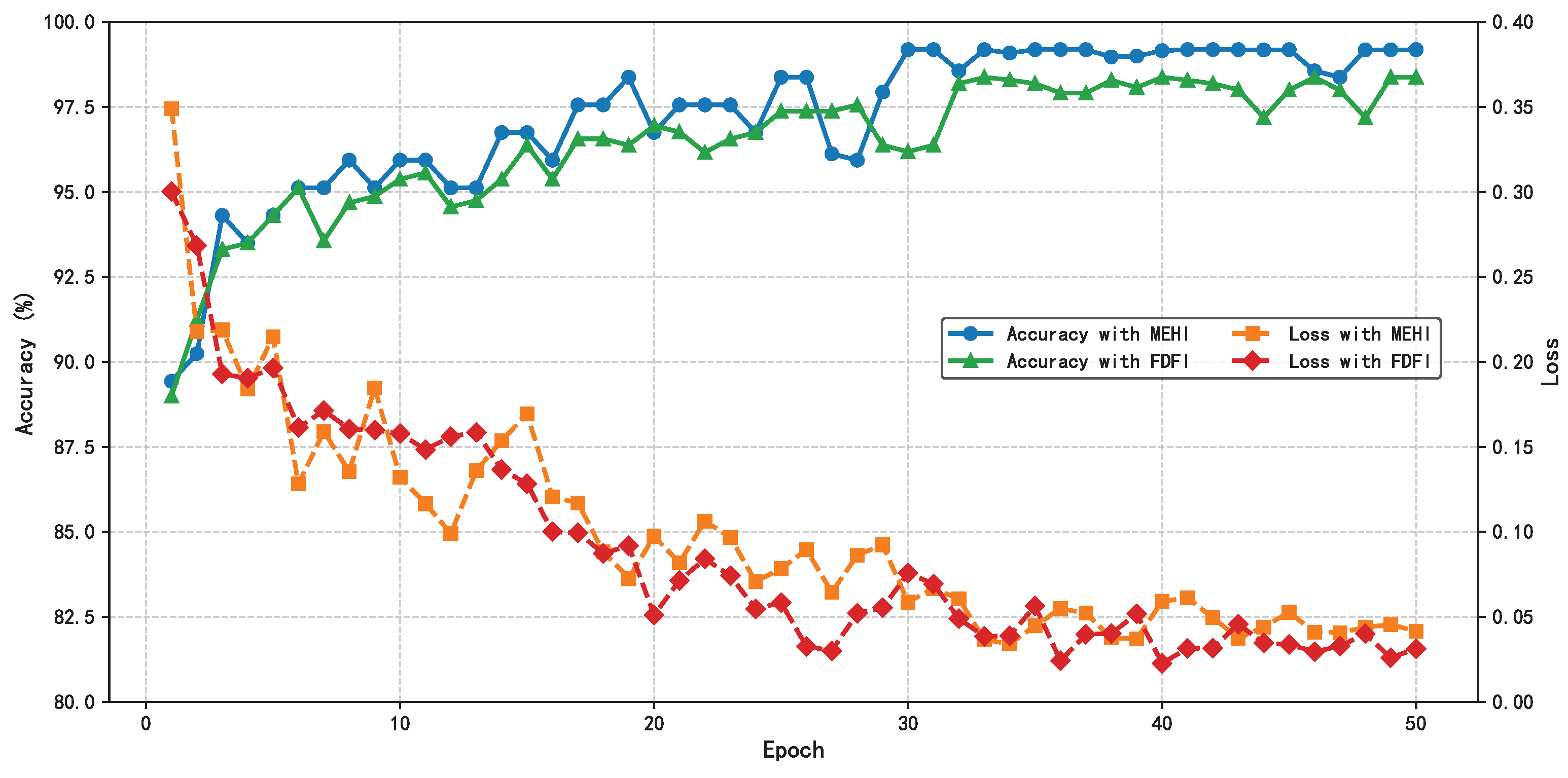
Like the HIE-MSTARLNet model using MEHIs, in the training process of training the HIE-MSTARLNet model using frequency-domain fusion images, the same parameters, training strategy, and loss function are used, and the two models are trained using data-enhanced scenarios, which are shown in
Figure 11. It can be seen that the HIE-MSTARLNet model using frequency-domain fused images converges more slowly and is somewhat less accurate than the HIE-MSTARLNet model using MEHIs. Therefore, the HIE-MSTARLNet model using MEHIs will be used as the final model in subsequent studies, and more detailed experiments will be conducted in the comparison experiments to illustrate the advantages of using the HIE-MSTARLNet model using MEHIs as the final model.
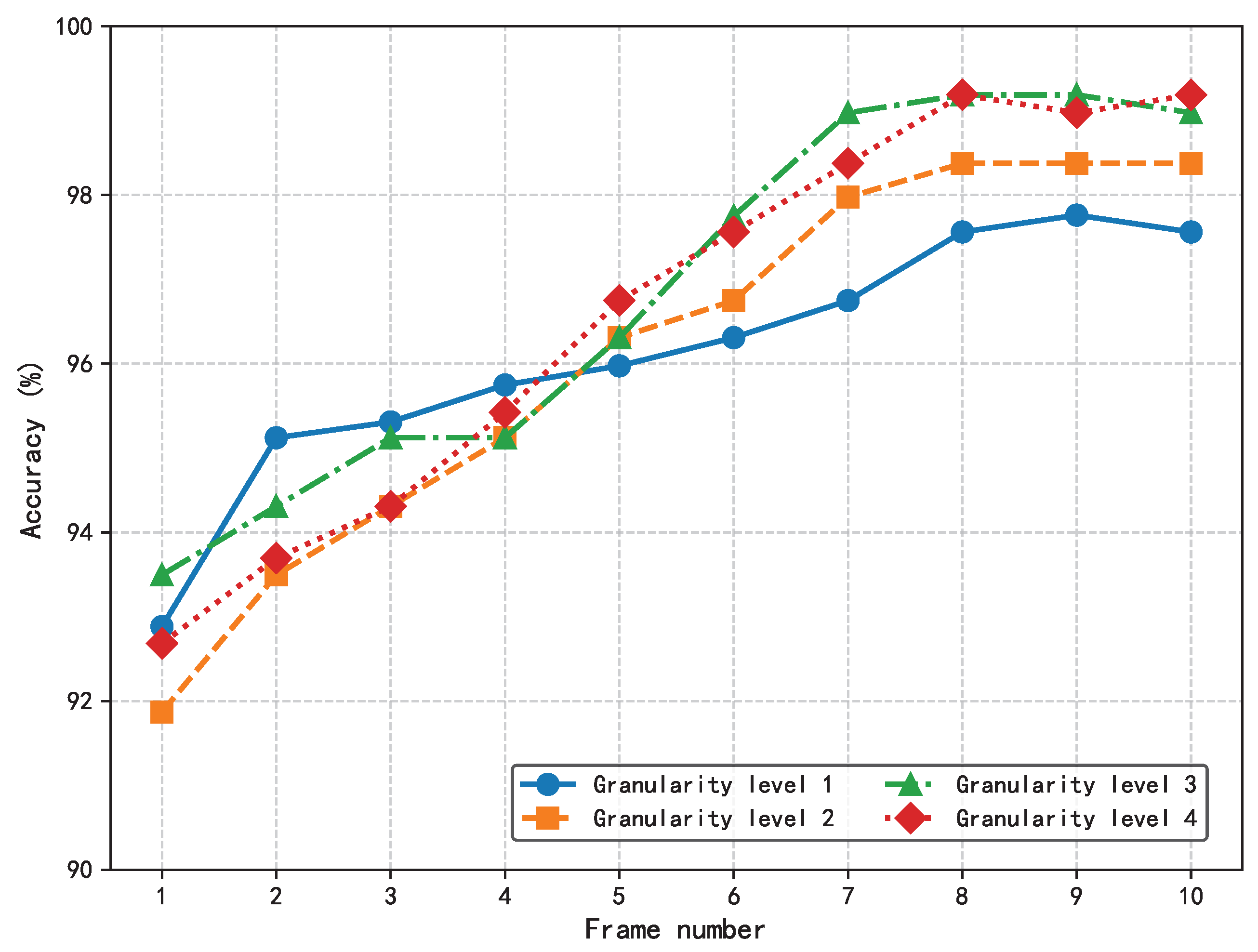
The effects of two key hyperparameters, the number of input frames and the granularity level, on the performance of the HIE-MSTARLNet model were investigated by varying the input frames and the granularity level, respectively, to test the classification accuracy of the model, as shown in
Figure 12.
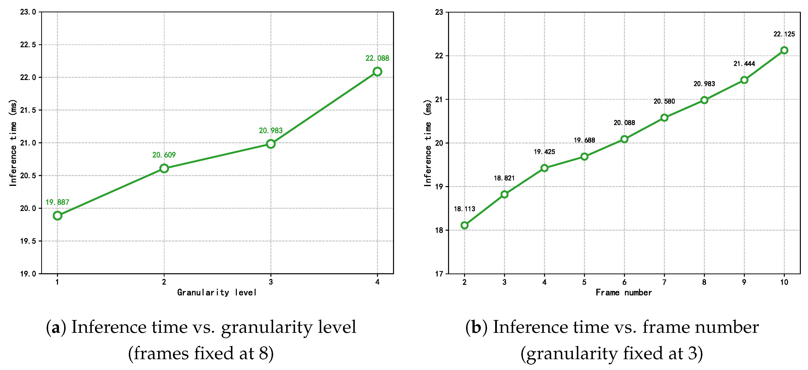
Consistent with the MFVNet model, the accuracy increases with the number of input frames. In addition, when the input frame sequence reaches a certain length, the accuracy increases with the increase in granularity level. Moreover, when the input reaches eight frames, accuracy stabilizes across different granularity levels, with no significant improvement from level 3 to level 4. To more accurately understand the influence of the number of sample frames and the number of granularity levels on the proposed model, the inference time of the proposed model is tested by changing the number of sample frames and the number of granularity levels, and the following experiments are set up to test the model. Firstly, the value of the input frames is fixed at eight, and the inference time of the model is tested at different granularity levels so that we can understand the effect of the change in granularity level on the inference time of the model, as shown in
Figure 13a. It can be seen that when the granularity level increases, it has a significant effect on the reasoning time of the proposed model.
Then, the number of granularity level is fixed to three to test the inference time of the model when inputting different sample frames to understand the effect of different sample frames on the inference time of the model; in this experiment, the model structure is only tested for the time series with sample frames from 2 to 10.
Figure 13b shows that when the input sample frames gradually increase, the model’s sample inference time also increases significantly.
In summary, while increasing both the number of sample frames and the number of granularity levels brings about an increase in the accuracy rate, it is accompanied by an increase in the inference time, which affects real-time detection in welding. Therefore, the number of input frames and the granularity level of the model were finally set to eight and three, respectively, to ensure accuracy while taking into account the inference time.
4.5. Stability Evaluation via Repeated Experiments and Cross-Validation
To assess the robustness of our model, we performed five independent training–validation–testing runs on the same data split, each with a different random seed. For each run, we recorded accuracy, precision, recall, the F1-score and the inference time. We then computed the sample’s mean (
) and standard deviation (
), as well as the 95% confidence interval (CI), under a normality assumption (The results are summarized in
Table 4):
4.6. Multi-Defect Extension of the WELDPOOL Dataset
On top of the original WELDPOOL dataset, which contained only 1200 porosity defect samples, we added 678 burn-through and 678 lack-of-fusion samples (see
Figure 14), resulting in a total of 2556 samples. We performed five independent training runs on this expanded dataset, achieving an average accuracy of 97.459%.
Table 5 presents the mean (
), standard deviation (
), and 95% confidence intervals for accuracy, precision, recall, and the F1-score to evaluate the stability of the model’s performance.
5. Discussion
This study addresses challenges in welding defect detection, including the limited interpretability of deep learning models, restricted real-time performance, and interclass similarity issues, by proposing a hybrid-enhanced multi-granularity spatiotemporal representation learning algorithm (HIE-MSTARLNet). By integrating temporal dynamic modeling, handcrafted feature enhancement, and a multi-granularity attention mechanism, the model achieves enhanced interpretability and inference efficiency without sacrificing detection accuracy. Firstly, a Temporal Shift Module (TSM) is embedded within the MobileNetV2 backbone to progressively capture the short-term dynamic features of molten pool images, including pixel-level shifts at shallow layers and motion patterns at deep layers—effectively modeling the temporal evolution of the molten pool. Compared to traditional 3D convolutional or Transformer-based approaches, TSM significantly reduces computational complexity, meeting the real-time requirements of industrial scenarios. Simultaneously, we propose the Molten Pool Edge History Image (MEHI) generation method that combines the Histogram of Oriented Gradient (HOG) and Scale-Invariant Feature Transform (SIFT) features to extract long-term spatial structural information from the molten pool images. These features are compressed using Principal Component Analysis (PCA) for dimensionality reduction. By concatenating handcrafted and deep learning features, the model enhances interpretability regarding physical molten pool characteristics (e.g., texture anomalies and contour distortion) while mitigating the risk of overfitting caused by reliance on single-feature types. Next, we design a Multi-granularity Attention Feature Aggregation module (MAFA). This module first selects key interference-free frames via cross-frame attention, then generates features at different granularity levels through grouped pooling. Attention mechanisms are subsequently applied to these multi-granularity features, adaptively fusing spatiotemporal features (global structure and local details) and replacing traditional hybrid attention mechanisms. The experimental results demonstrate that MAFA significantly improves classification accuracy, reduces redundancy in multi-scale features, and optimizes computational efficiency. Parameter analysis determined the optimal number of input frames (eight frames) and granularity levels (three levels). Ablation experiments verified the effectiveness of the TSM, MAFA, and handcrafted feature modules. When evaluated solely on porosity defect detection, HIE-MSTARLNet achieved an accuracy of 99.187%. When burn-through and lack-of-fusion defects were added, HIE-MSTARLNet’s remained at 97.459%. Visual analysis further indicates that the model focuses on variations in light spots and texture within the central molten pool surface region, contrasting traditional contour-based attention, thus providing new insights for defect attribution.
While our model has shown high performance and good real-time capabilities on our custom dataset, some limitations remain. The current algorithm focuses on identifying potential porosity defects, and further exploration is needed to extend its applicability to identify a broader range of welding defects. Although we have extended beyond porosity defects to include burn-through and lack-of-fusion defects, the total dataset remains limited to 2556 samples. Deep learning models typically benefit from larger datasets to enhance their generalization and robustness. Future research should further explore model improvements, investigate a broader spectrum of welding defects and molten pool characteristics, and collect more diverse and larger-scale welding defect video datasets to improve model performance.


 and
and 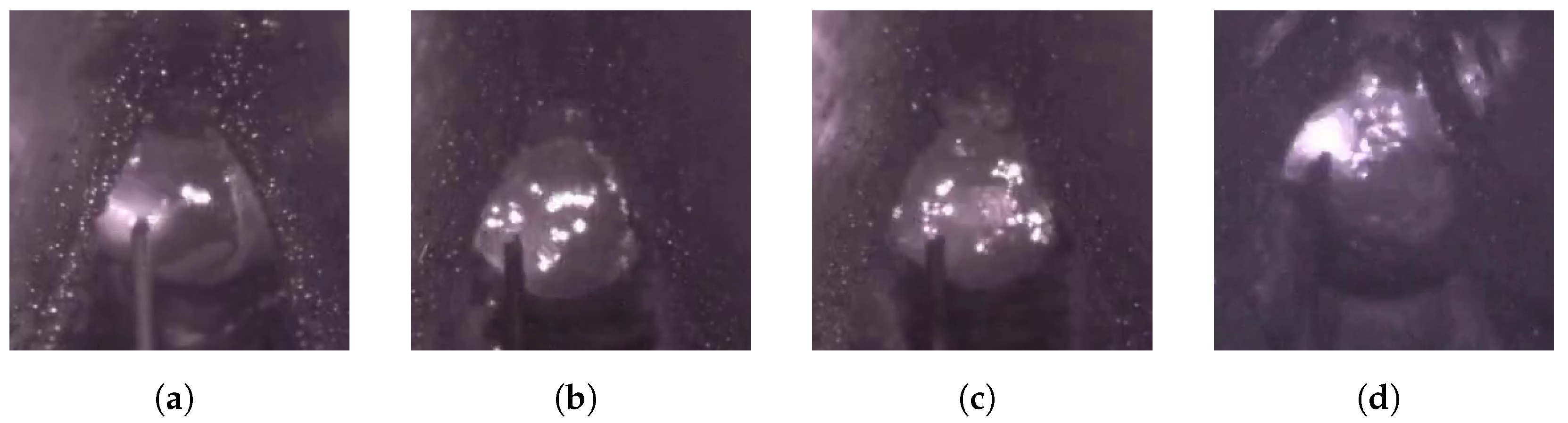


