
Computationally Efficient Impact Estimation of Coil Misalignment for Magnet-Free Cochlear Implants


Abstract
1. Introduction
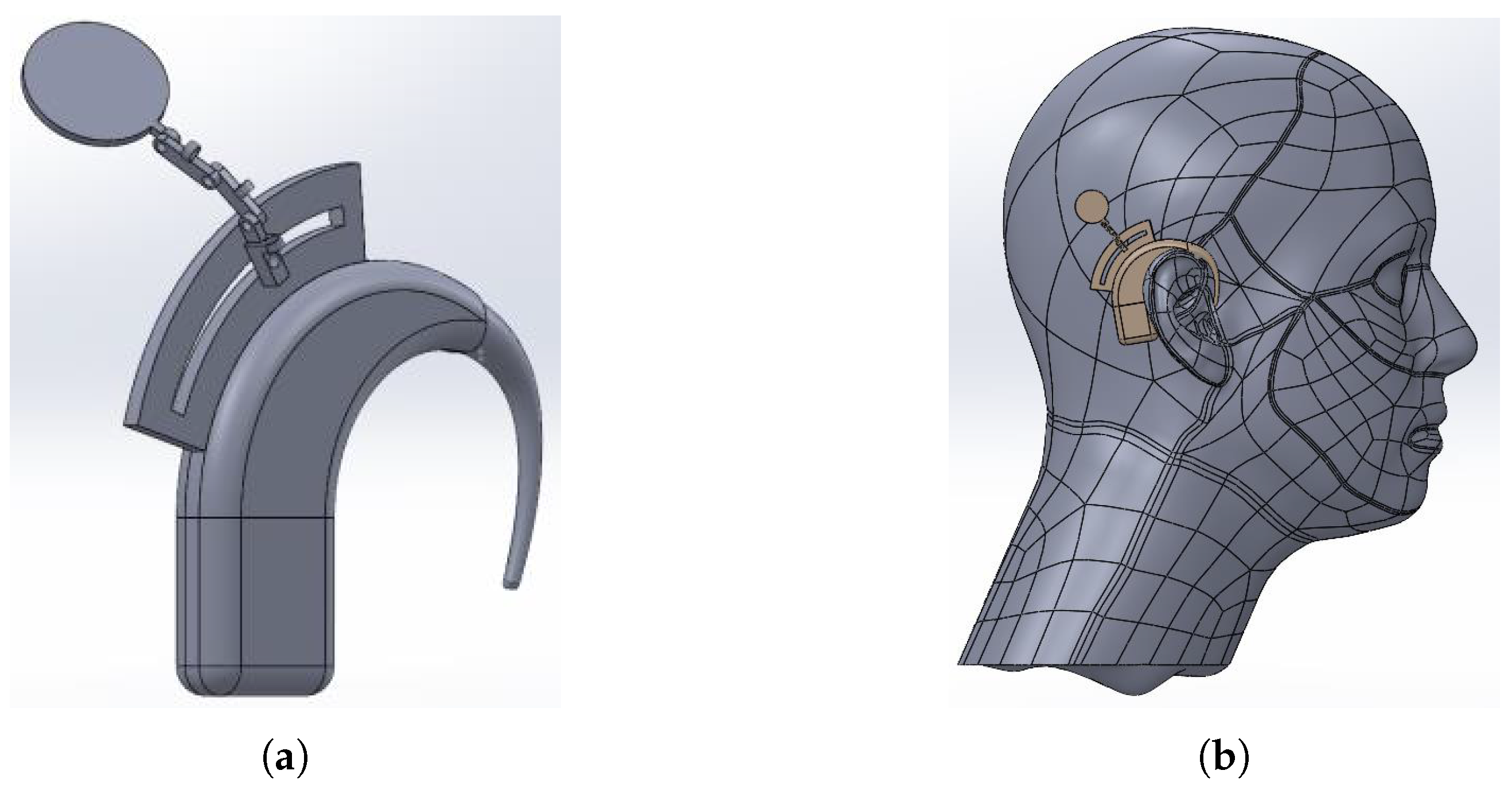
1.1. A Cochlear Implant
1.2. Challenge
2. Materials and Methods
2.1. The Coupling Coefficient
2.1.1. The Self-Inductance of a Coil
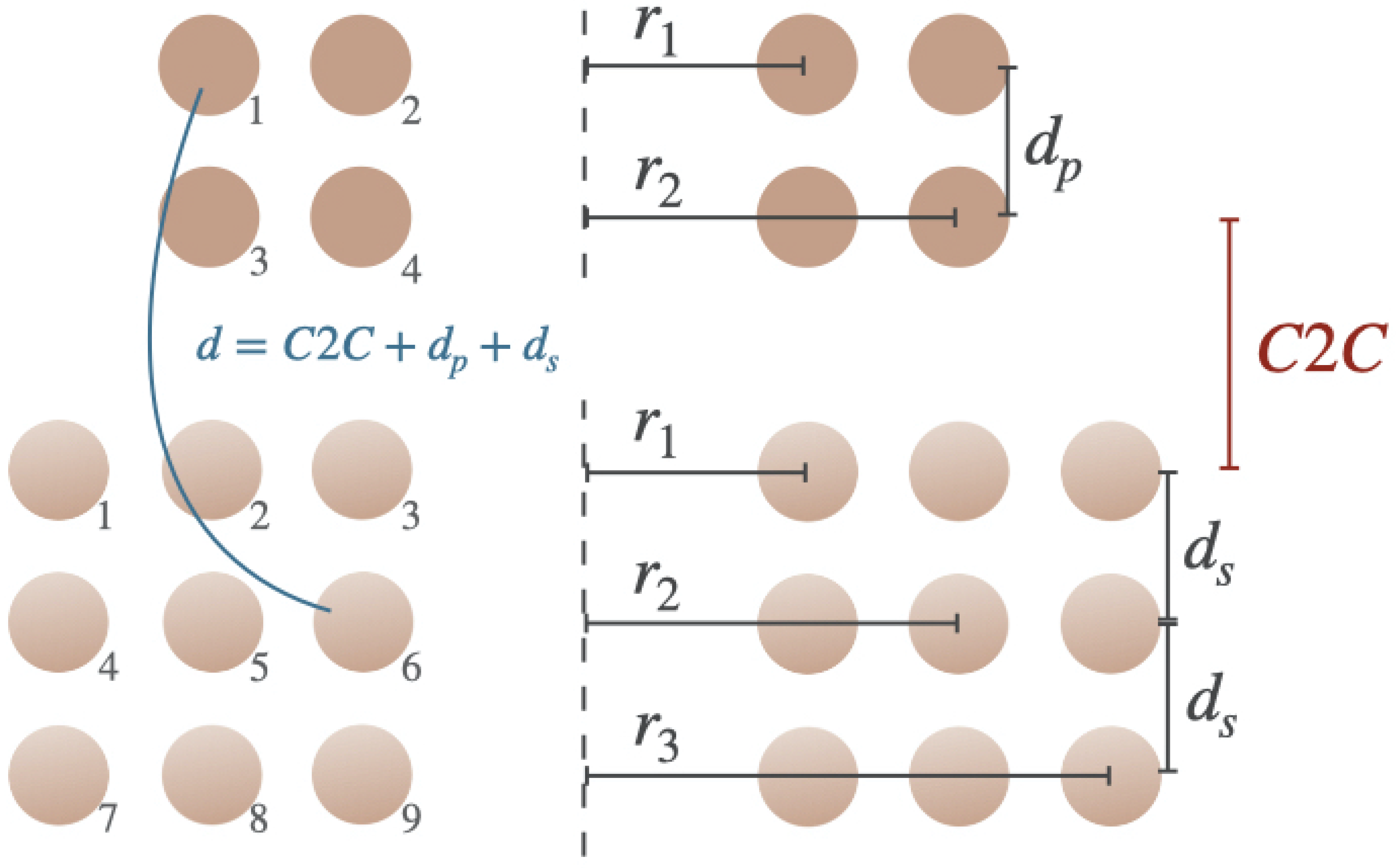
2.1.2. Mutual Inductance Between Two Aligned Coils
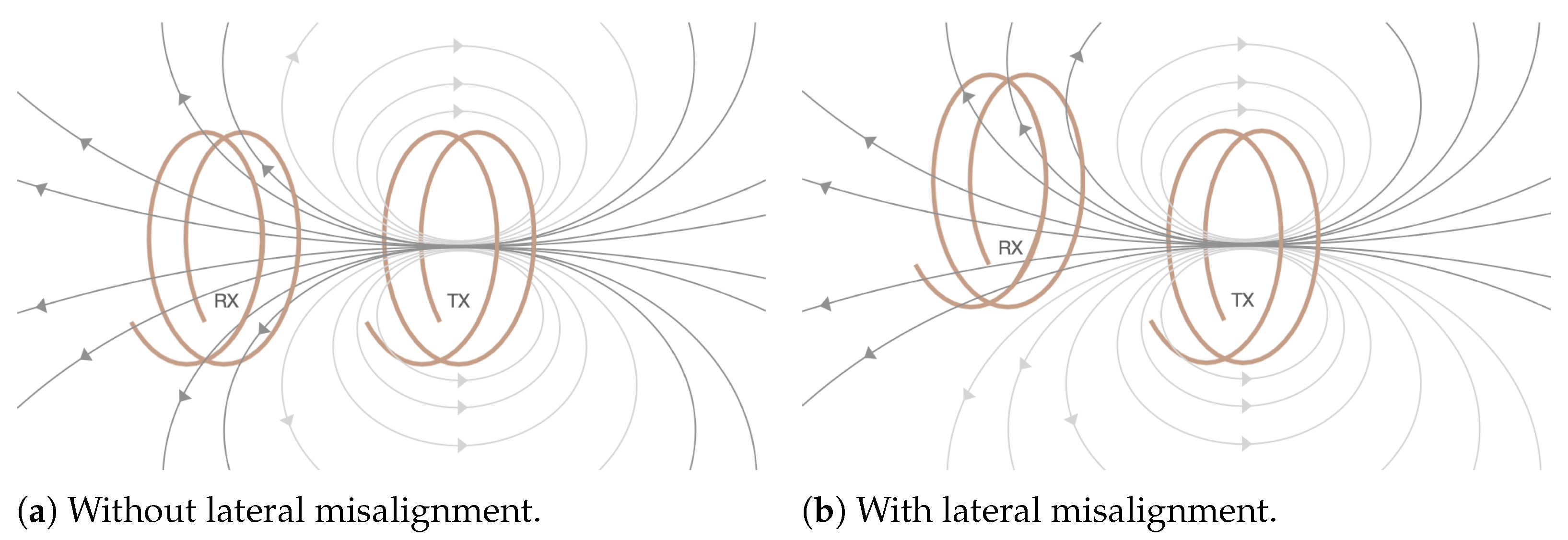
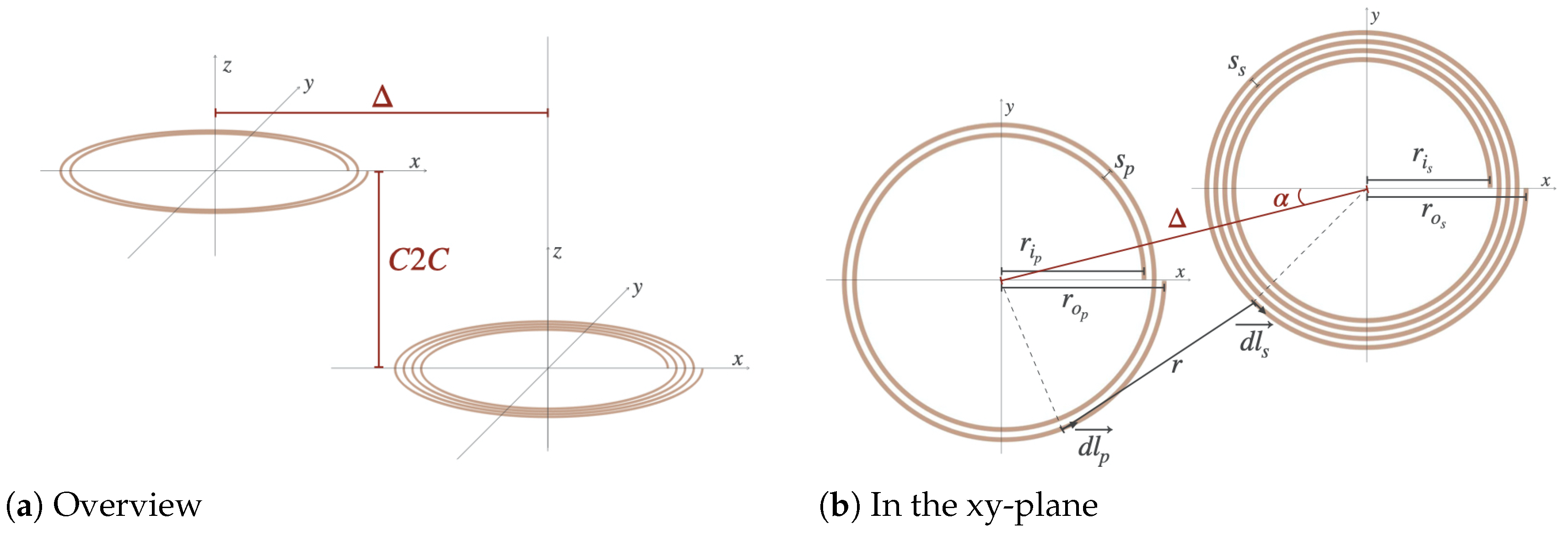
2.1.3. Mutual Inductance Between Two Coils with Lateral and/or Angular Misalignment
2.2. Literature Review
2.2.1. First Approach (Anele et al. [20] and Babic et al. [21])
2.2.2. Second Approach (Liu et al. [22])
2.3. Methodology
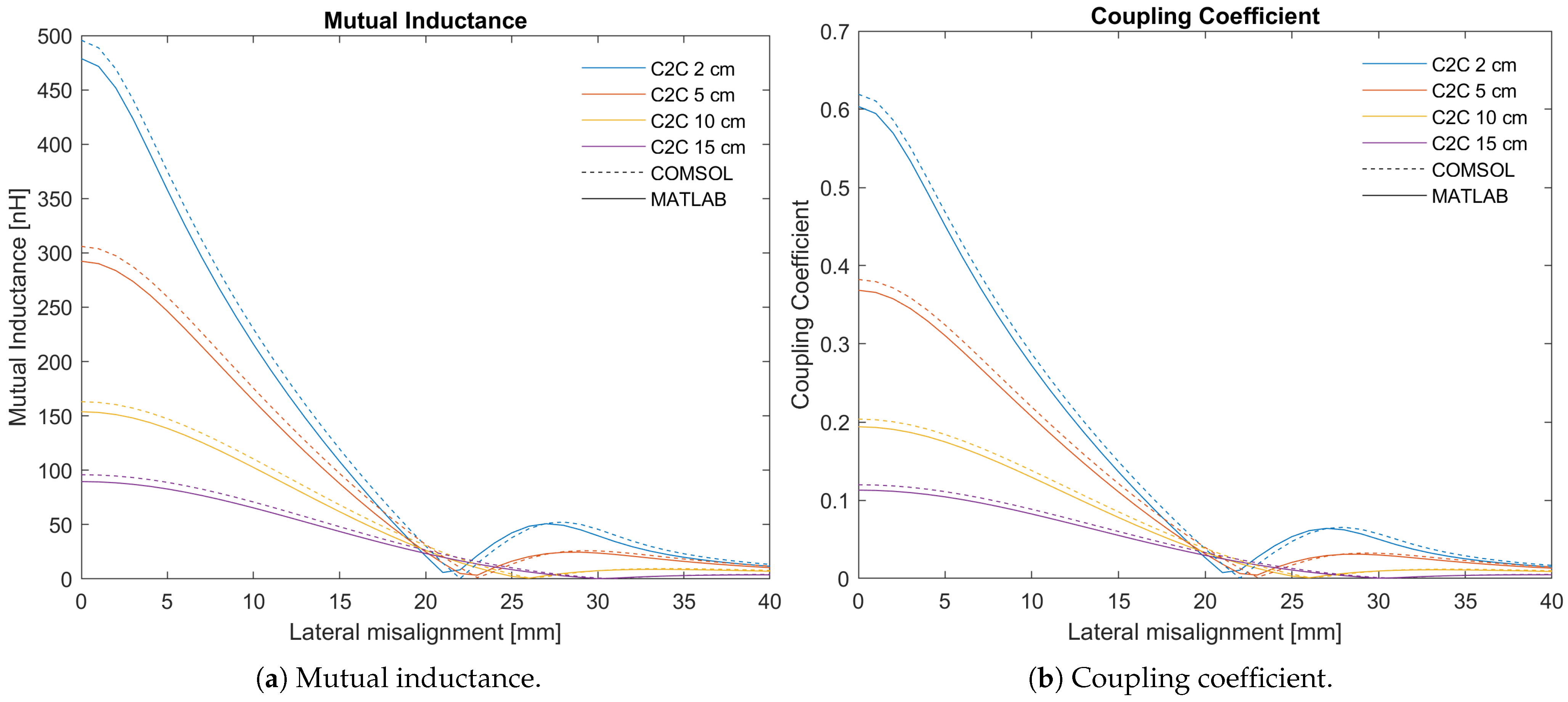
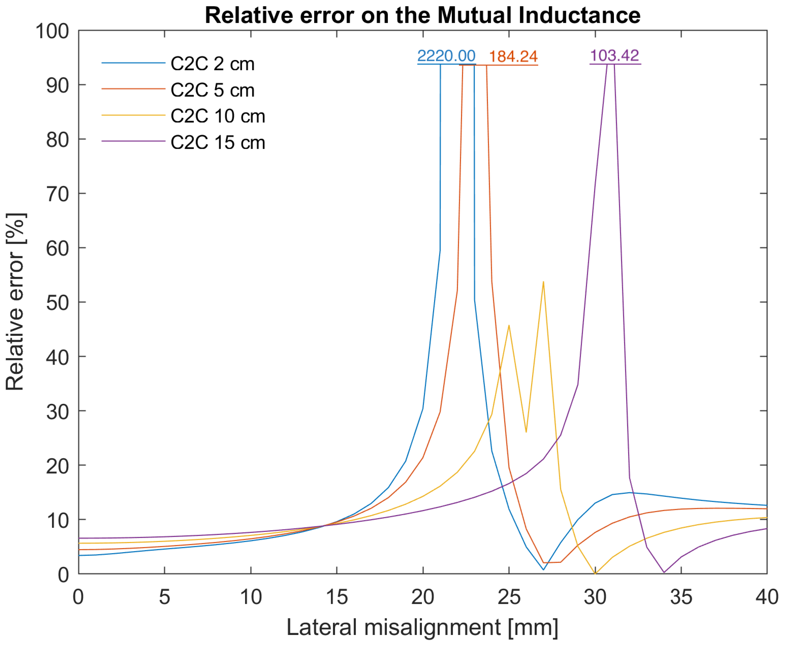
3. Results and Validation
4. Discussion
5. Conclusions
Author Contributions
Funding
Institutional Review Board Statement
Informed Consent Statement
Data Availability Statement
Conflicts of Interest
Abbreviations
| BTE | Behind-the-Ear |
| CI | Cochlear Implant |
| C2C | Coil-to-Coil |
| FEA | Finite Element Analysis |
| MRI | Magnetic Resonance Imaging |
| SFT | Skin Flap Thickness |
| TEDZ | Transmission Efficiency Dead-Zone |
Appendix A
| Algorithm A1: Self-inductance of a coil: self_inductance |
Input: - Array of radii r - Wire radius a - Number of layers l - Distance between the layers d Output: - Self-inductance I Initialisation: Set N = size of r Set = Preallocate , matrix NxN 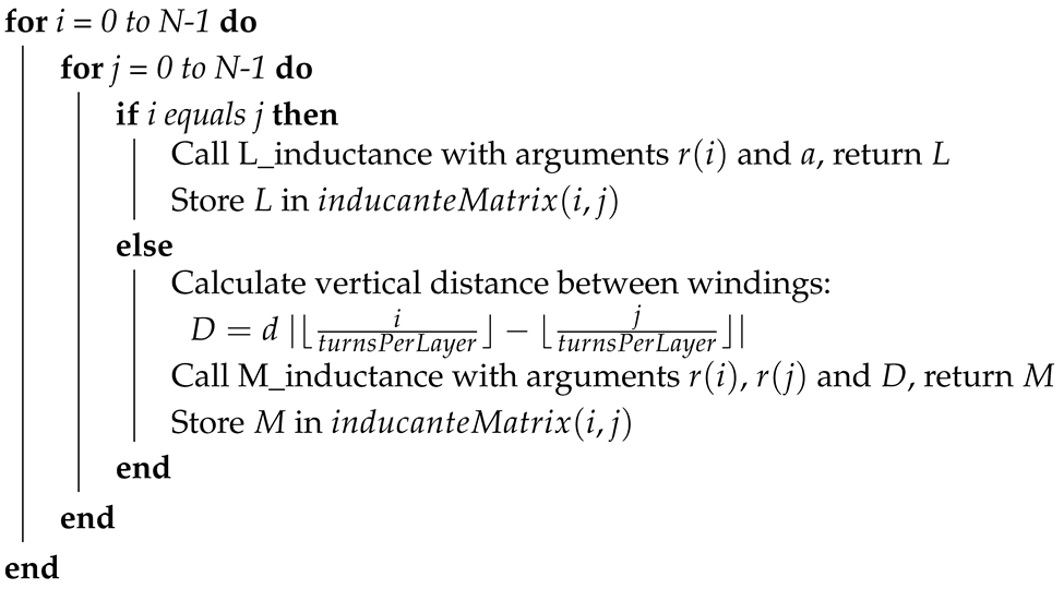 Calculate self-inductance: |
| Algorithm A2: Inductance for one circular winding: L_inductance |
Input: - Radius r - Wire radius a Output: - Inductance L Initialisation: Set Calculate inductance: |
| Algorithm A3: Mutual inductance between two windings: M_inductance |
Input: - Radius of winding 1 - Radius of winding 2 - Distance between the windings d Output: - Mutual inductance M Initialisation: Set Set Call ellipke with arguments and , return K and E Calculate mutual inductance: |
| Algorithm A4: Mutual inductance between two coils: mutual_inductance |
Input: - Array of radii of the primary coil - Number of layers of the primary coil - Distance between the windings of the pimary coil - Array of radii of the secondary coil - Number of layers of the secondary coil - Distance between the windings of the secondary coil - distance between the two coils c Output: - Mutual inductance between the two coils Initialisation: Set N = size of Set to Set M = size of Set to Preallocate , matrix NxM 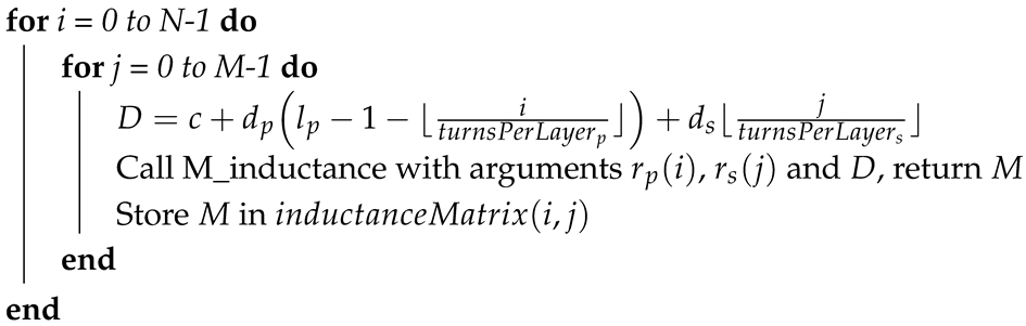 Calculate mutual inductance: |
| Algorithm A5: Mutual inductance between two coils with lateral misalignment: mutual_inductance_ |
Input: - Array of radii of the primary coil - Number of layers of the primary coil - Distance between the windings of the primary coil - Array of radii of the secondary coil - Number of layers of the secondary coil - Distance between the windings of the secondary coil - distance between the two coils c - Lateral misalignment between the coils Output: - Mutual inductance between the two coils Initialisation: Set Set N = size of Set to Set M = size of Set to Preallocate , matrix NxM 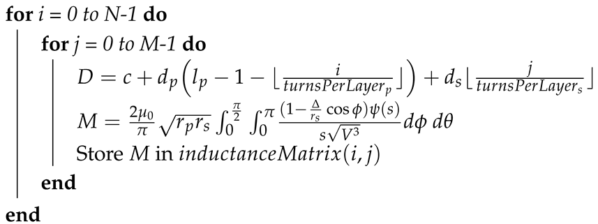 Calculate mutual inductance: |
| Algorithm A6: Coupling coefficient between two coils with lateral misalignment |
Input: - Array of radii of the primary coil - Wire radius of the primary coil - Number of layers of the primary coil - Distance between the windings of the primary coil - Array of radii of the secondary coil - Wire radius of the secondary coil - Number of layers of the secondary coil - Distance between the windings of the secondary coil - Array of distances between the two coils c - Array of lateral misalignments between the coils Output: - Matrix K of coupling coefficient for a range of and between the two coils Initialisation: Set = size of c Set = size of Call L_inductance with arguments , , and , return Call L_inductance with arguments , , and , return Preallocate K, matrix x 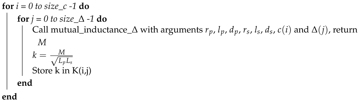 |
References
- Rajamanickam, N.; Ramachandaramurthy, V.K.; Gono, R.; Bernat, P. Misalignment-tolerant wireless power transfer for high endurance IoT sensors using UAVs and nonlinear resonant circuits. Results Eng. 2025, 26, 104879. [Google Scholar] [CrossRef]
- Van Mulders, J.; Boeckx, S.; Cappelle, J.; Van der Perre, L.; De Strycker, L. UAV-based solution for extending the lifetime of IoT devices: Efficiency, design and sustainability. Front. Commun. Netw. 2024, 5, 1341081. [Google Scholar] [CrossRef]
- Viqar, S.; Ahmad, A.; Kirmani, S.; Rafat, Y.; Hussan, M.R.; Alam, M.S. Modelling, simulation and hardware analysis of misalignment and compensation topologies of wireless power transfer for electric vehicle charging application. Sustain. Energy Grids Netw. 2024, 38, 101285. [Google Scholar] [CrossRef]
- Debnath, T.; Majumder, S.; De, K. High-efficiency coil design for wireless power transfer: Mitigating misalignment challenges in transportation. Energy 2025, 325, 135929. [Google Scholar] [CrossRef]
- Brownell, W.E. How the ear works—Nature’s solutions for listening. Volta Rev. 1997, 99, 9–28. [Google Scholar] [PubMed] [PubMed Central]
- Cochlear Ltd. How Hearing Works. 2019. Available online: https://www.cochlear.com/us/en/home/diagnosis-and-treatment/diagnosing-hearing-loss/how-hearing-works (accessed on 30 June 2021).
- Cochlear Ltd. Types and Causes of Hearing Loss. 2019. Available online: https://www.cochlear.com/us/en/home/diagnosis-and-treatment/diagnosing-hearing-loss/types-and-causes-of-hearing-loss (accessed on 30 June 2021).
- Deep, N.; Jethanamest, E.D.D.; Carlson, M. Cochlear Implantation: An Overview. J. Neurol. Surg. Part Skull Base 2018, 80, 169–177. [Google Scholar] [CrossRef] [PubMed]
- Cochlear Ltd. About Cochlear Implants. 2019. Available online: https://www.cochlear.com/us/en/corporate/media-center/about-cochlear-implants (accessed on 30 June 2021).
- Cochlear Ltd. How Cochlear Implants Work. 2019. Available online: https://www.cochlear.com/us/en/home/diagnosis-and-treatment/how-cochlear-solutions-work/cochlear-implants/how-cochlear-implants-work/how-cochlear-implants-work (accessed on 30 June 2021).
- Dupont, P. (KU Leuven Campus Group T, Leuven, Belgium) Information Processing in Health Technology, Basics of Medical Imaging, Part: Medical Resonance Imaging. B-KUL-T5IPHT. Class Lecture. 2020. Available online: https://onderwijsaanbod.kuleuven.be/syllabi/e/T5IPHTE.htm#activetab=doelstellingen_idm5676816 (accessed on 30 June 2021).
- Giancoli, D.C. Physics for Scientists and Engineers with Modern Physics; Prentice-Hall: Englewood Cliffs, NJ, USA, 2008. [Google Scholar]
- Jansson, K.F.; Hakansson, B.; Reinfeldt, S.; Taghavi, H.; Eeg-Olofsson, M. MRI Induced Torque and Demagnetization in Retention Magnets for a Bone Conduction Implant. IEEE Trans. Biomed. Eng. 2014, 61, 1887–1893. [Google Scholar] [CrossRef] [PubMed]
- Panych, L.P.; Madore, B. The physics of MRI safety. J. Magn. Reson. Imaging 2018, 47, 28–43. [Google Scholar] [CrossRef] [PubMed]
- Delfino, J.G.; Woods, T.O. New Developments in Standards for MRI Safety Testing of Medical Devices. Curr. Radiol. Rep. 2016, 4, 28. [Google Scholar] [CrossRef]
- Kim, B.G.; Kim, J.W.; Park, J.J.; Kim, S.H.; Kim, H.N.; Choi, J.Y. Adverse Events and Discomfort During Magnetic Resonance Imaging in Cochlear Implant Recipients. JAMA Otolaryngol. Head Neck Surg. 2015, 141, 45–52. [Google Scholar] [CrossRef] [PubMed]
- Tenllado, I.C.C.; Cabrera, A.T. Encyclopedia of Electrical and Electronic Power Engineering; Elsevier: Oxford, UK, 2023. [Google Scholar]
- Rosa, E.B. The self and mutual inductances of linear conductors. Bull. Bur. Stand. 1908, 4, 301–344. [Google Scholar] [CrossRef]
- Barrios, J. A Brief History of Elliptic Integral Addition Theorems. Rose-Hulman Undergrad. Math. J. 2009, 10, 2. [Google Scholar]
- Anele, A.O.; Hamam, Y.; Chassagne, L.; Linares, J.; Alayli, Y.; Djouani, K. Computation of the Mutual Inductance between Air-Cored Coils of Wireless Power Transformer. J. Phys. 2015, 633, 12011. [Google Scholar] [CrossRef]
- Babic, S.; Sirois, F.; Akyel, C.; Girardi, C. Mutual Inductance Calculation Between Circular Filaments Arbitrarily Positions in Space: Alternative to Grover’s Formula. IEEE Trans. Magn. 2010, 46, 3591–3600. [Google Scholar] [CrossRef]
- Liu, S.; Su, J.; Lai, J. Accurate Expressions of Mutual Inductance and Their Calculation of Archimedean Spiral Coils. Energies 2019, 12, 2017. [Google Scholar] [CrossRef]
- Grover, F.W. The Calculation of the Mutual Inductance of Circular Filaments in Any Desired Positions. Proc. Ire 1944, 32, 620–629. [Google Scholar] [CrossRef]
- Mohdeb, N. Comparative Study of Circular Flat Spiral Coils Structure Effect on Magnetic Resonance Wireless Power Transfer Performance. Prog. Electromagn. Res. Pier 2020, 94, 119–129. [Google Scholar] [CrossRef]


| MATLAB [] | FEA [] | [%] | |
|---|---|---|---|
| 537.88 | 540.13 | 0.42 | |
| 1169.55 | 1185.90 | 1.38 |
Disclaimer/Publisher’s Note: The statements, opinions and data contained in all publications are solely those of the individual author(s) and contributor(s) and not of MDPI and/or the editor(s). MDPI and/or the editor(s) disclaim responsibility for any injury to people or property resulting from any ideas, methods, instructions or products referred to in the content. |
© 2025 by the authors. Licensee MDPI, Basel, Switzerland. This article is an open access article distributed under the terms and conditions of the Creative Commons Attribution (CC BY) license (https://creativecommons.org/licenses/by/4.0/).
Share and Cite
Boeckx, S.; Polfliet, P.; De Strycker, L.; Van der Perre, L. Computationally Efficient Impact Estimation of Coil Misalignment for Magnet-Free Cochlear Implants. Sensors 2025, 25, 4379. https://doi.org/10.3390/s25144379
Boeckx S, Polfliet P, De Strycker L, Van der Perre L. Computationally Efficient Impact Estimation of Coil Misalignment for Magnet-Free Cochlear Implants. Sensors. 2025; 25(14):4379. https://doi.org/10.3390/s25144379
Chicago/Turabian StyleBoeckx, Samuelle, Pieterjan Polfliet, Lieven De Strycker, and Liesbet Van der Perre. 2025. "Computationally Efficient Impact Estimation of Coil Misalignment for Magnet-Free Cochlear Implants" Sensors 25, no. 14: 4379. https://doi.org/10.3390/s25144379
APA StyleBoeckx, S., Polfliet, P., De Strycker, L., & Van der Perre, L. (2025). Computationally Efficient Impact Estimation of Coil Misalignment for Magnet-Free Cochlear Implants. Sensors, 25(14), 4379. https://doi.org/10.3390/s25144379