
Research on Three-Axis Vibration Characteristics and Vehicle Axle Shape Identification of Cement Pavement Under Heavy Vehicle Loads Based on EMD–Energy Decoupling Method


Abstract
Highlights
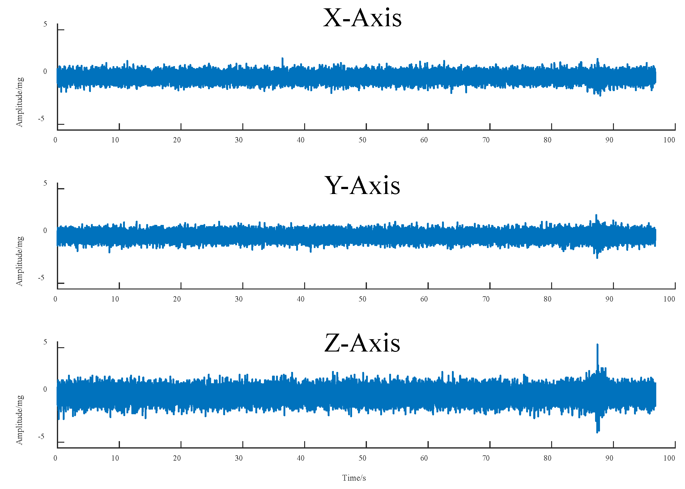
- Vertical (Z-axis) vibrations have the highest amplitude and frequency components, highlighting their key role in pavement response.
- EMD and STE analyses effectively identify axle impacts and enable accurate axle configuration recognition.
- The findings contribute to better pavement health monitoring and performance assessment under heavy vehicle loads.
- Provides a reliable method for axle identification, supporting infrastructure management and optimizing traffic flow.
Abstract
1. Introduction
2. Field Tests of Subgrade Soil Under Heavy-Duty Vehicle Load
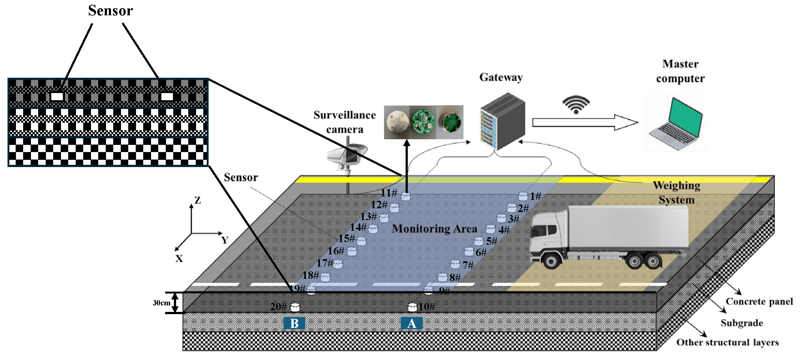
2.1. Three-Axis Vibration Monitoring System
2.2. Pavement Vibration Response Signal Acquisition
- (1)
- The performance of the sensors is critical for the experimental research. All sensors must be calibrated before being installed on-site, and comprehensive laboratory tests are conducted for their performance and stability;
- (2)
- Check the monitoring system line connection, pre-test to confirm that all sensor data acquisition function is normal;
- (3)
- Set the sampling frequency of 500 Hz following the initiation of data acquisition, while starting the camera to shoot the road vehicle information;
- (4)
- After the rear wheels of the vehicle pass through the 1# sensor arrangement array, wait for 30 s to click the End button and save the collection;
- (5)
- Synchronise the video, weighing system, and vibration data storage.
3. Methods and Principles of Data Analysis
3.1. Signal Noise Reduction Based on Smooth Wavelet Transform
3.2. EMD Decomposition
- (1)
- The difference between the number of zero crossing points and the number of extreme points of the IMF is at most one throughout the data series;
- (2)
- The local mean of the IMF at any moment should be zero.
3.3. Short-Term Energy Analysis
4. Discussion
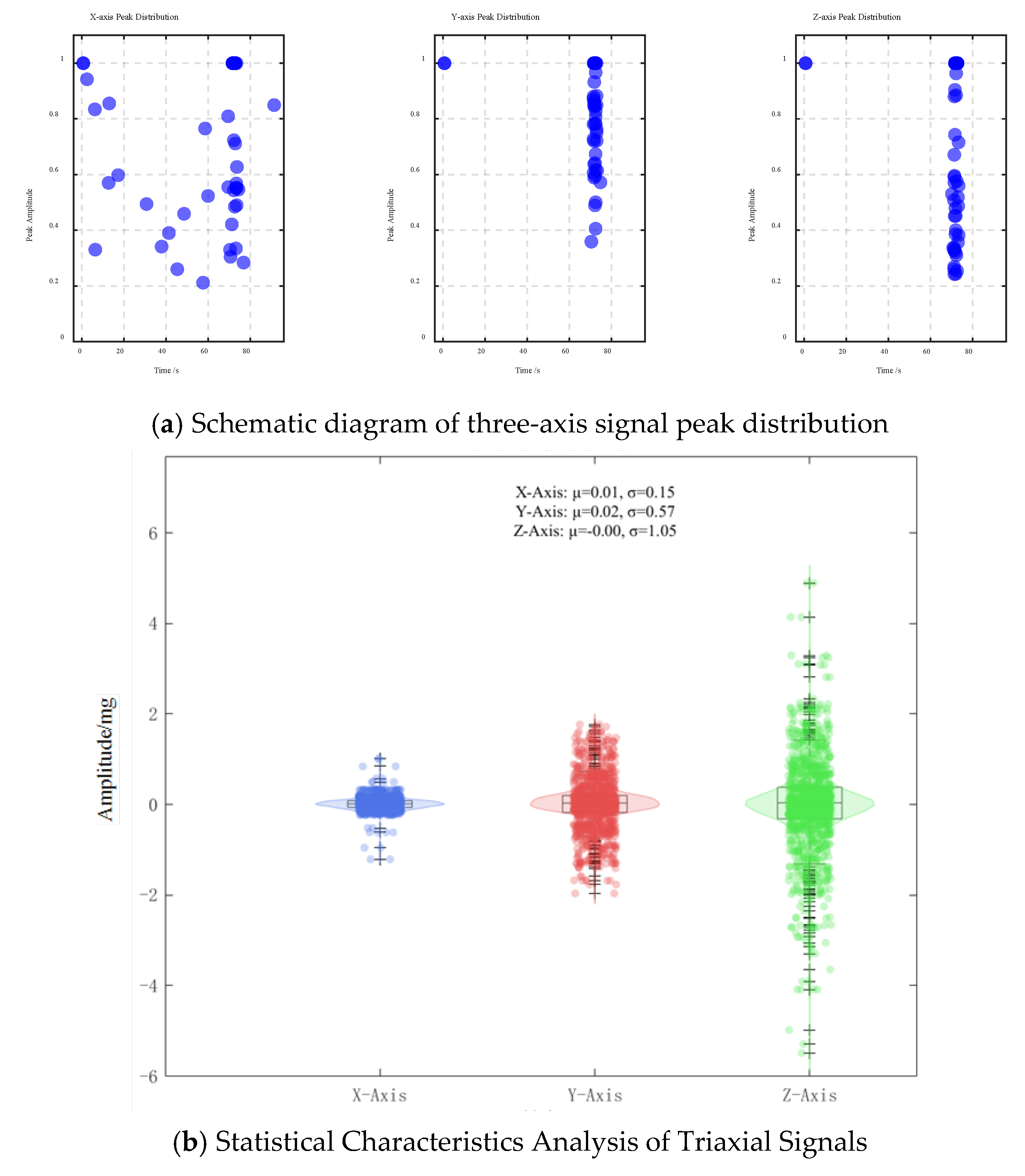
4.1. Three-Axis Characteristics of Vibration Response Signals
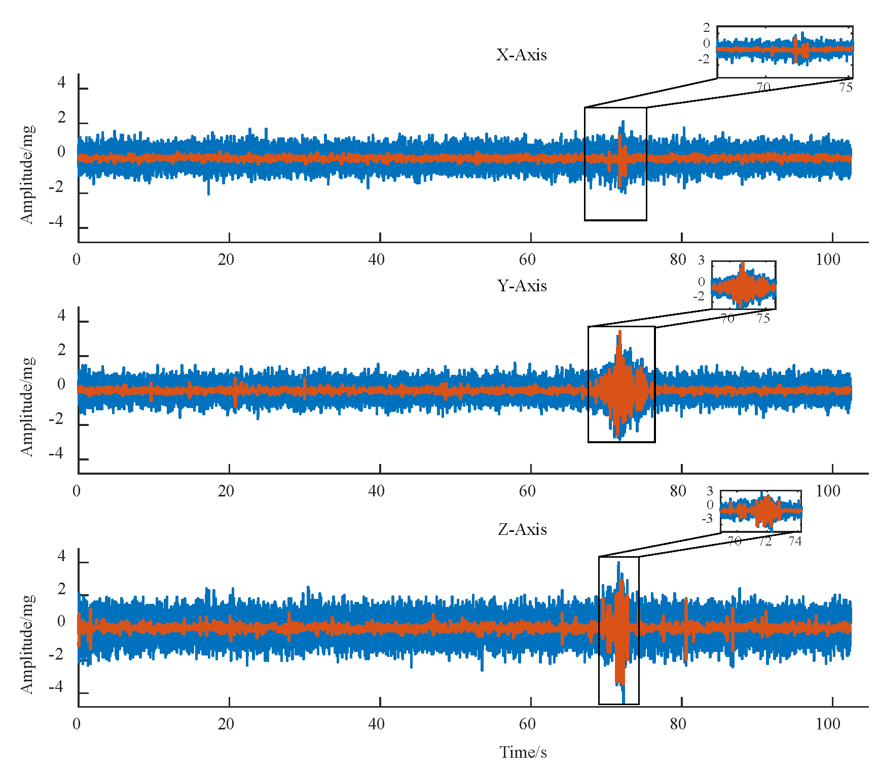
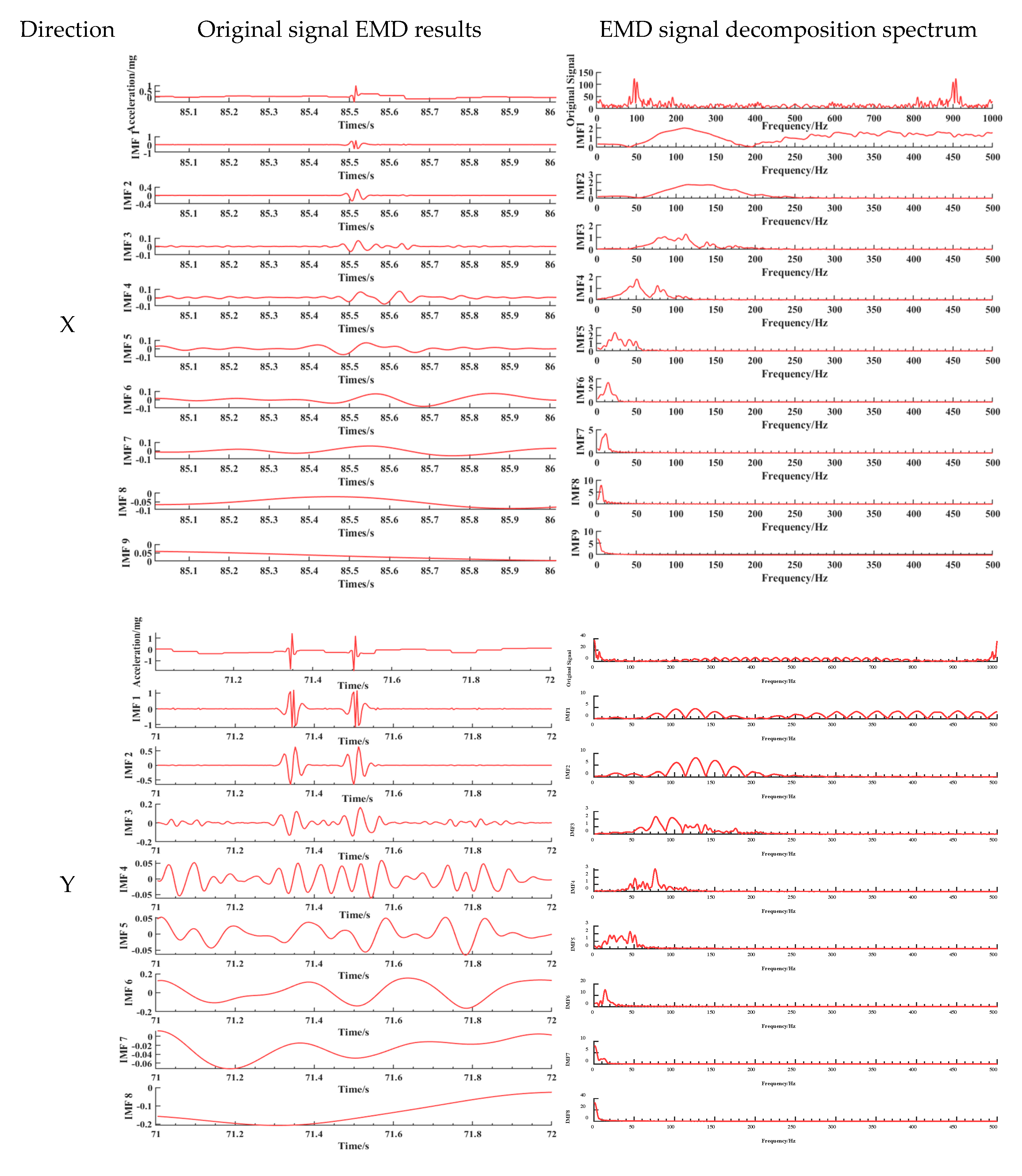
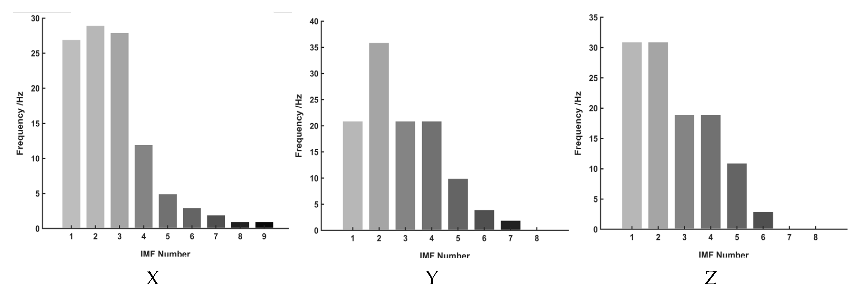
4.2. EMD-Based Triaxial Vibration Signal Characterization
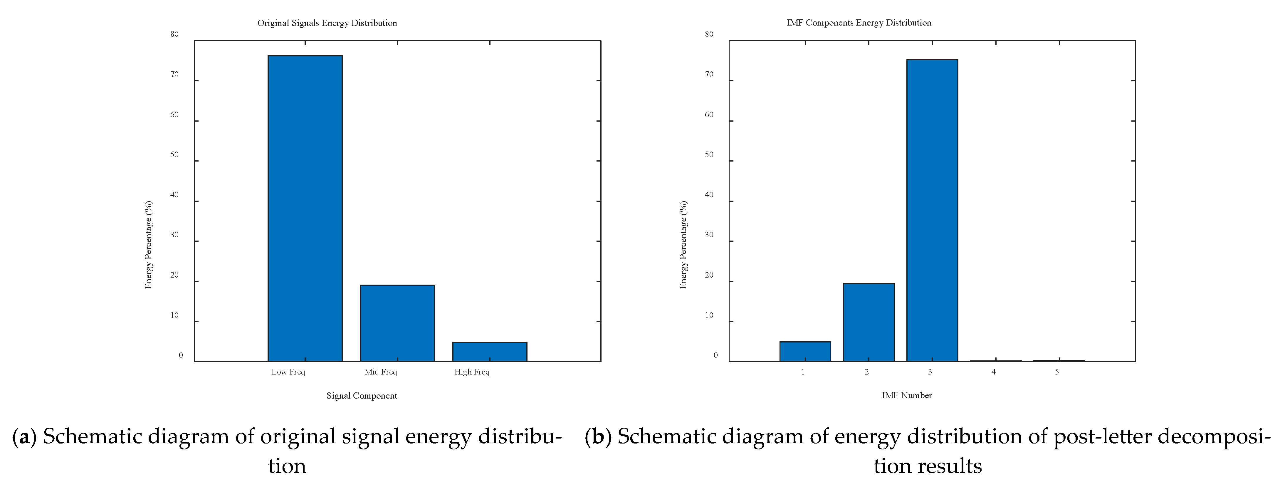
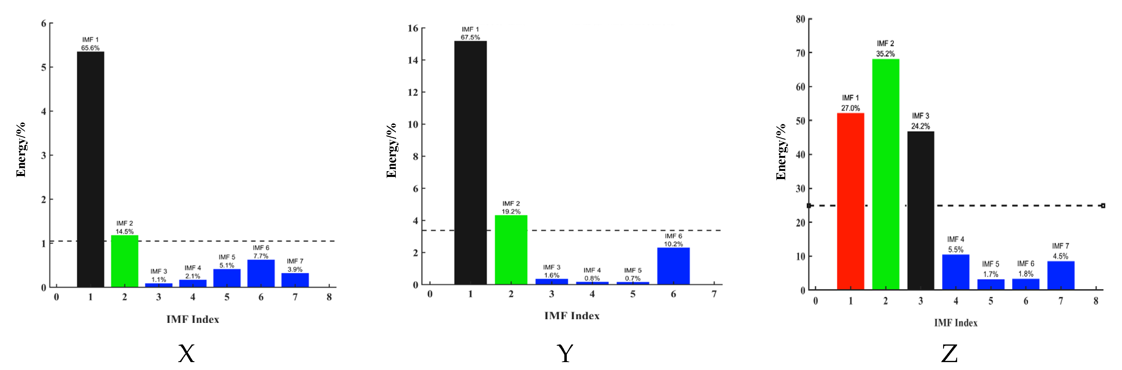
4.3. IMF Filtering
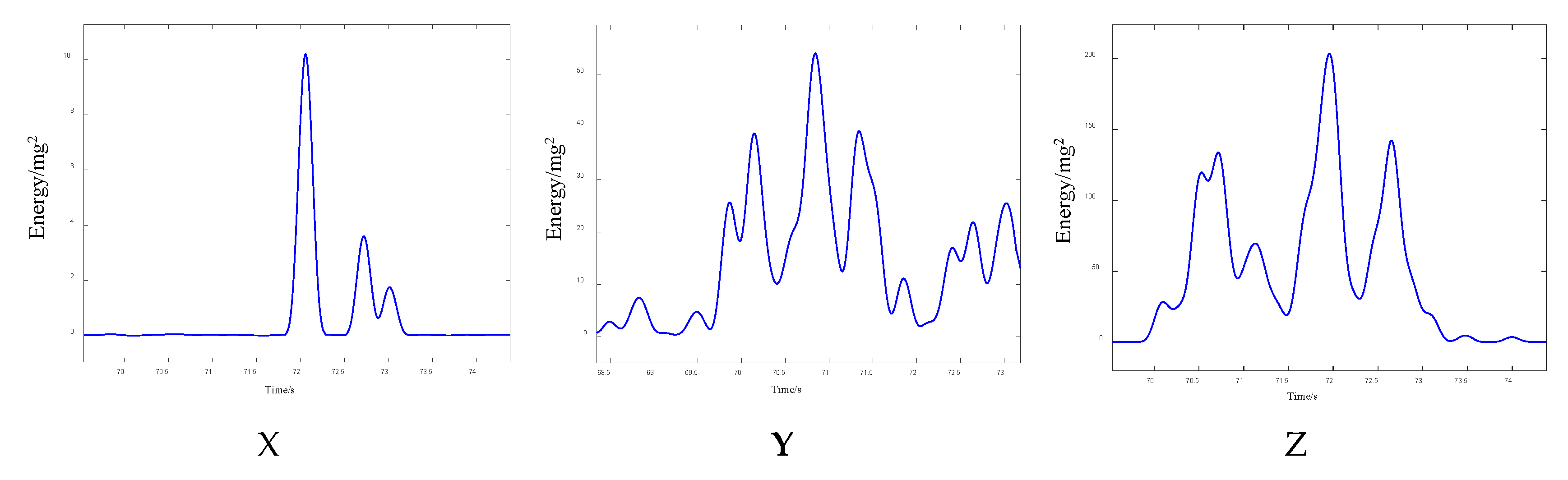
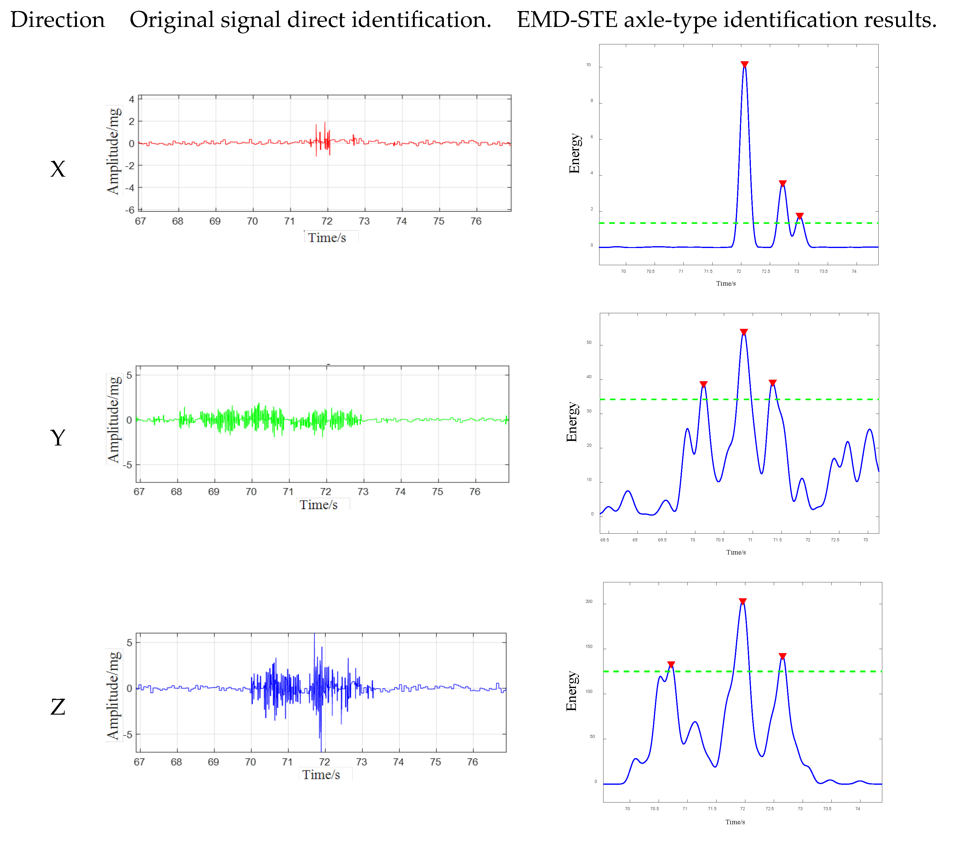
4.4. Vehicle Axle Type Recognition Based on Short-Time Energy Profile
- (1)
- Signal normalization
- (2)
- Sliding window segmentation
- (3)
- Spectrum leakage suppression
- (4)
- Short-term energy calculation
- (1)
- Minimum peak height: The amplitude of energy signals generated by different vehicles (no load/heavy load) and different axles (steering shaft/drive shaft) is quite different, and the signal baseline may fluctuate, so the fixed threshold is not effective. Therefore, this paper adopts an adaptive strategy based on the statistical characteristics of signals. The STE threshold is determined based on the global maximum peak value. First, find the global maximum peak on the short-time energy (STE) curve obtained. Then, by analysing the noise level, the height threshold for peak detection is set at 30% of the maximum peak value. This method can automatically adjust the threshold based on the overall energy level of the signal, ensuring that significant energy peaks caused by shaft impacts can be effectively distinguished from background noise and minor fluctuations. This approach avoids the bias that might be introduced by using a fixed absolute value threshold.
- (2)
- Minimum peak prominence: This parameter is crucial for distinguishing independent true axle peaks from shoulder peaks on the main peak or secondary energy peaks caused by vibration. It quantifies the significance of a peak with respect to its surrounding signal, requiring that an effective peak must have sufficient relative height within its local neighbourhood. In this paper, through empirical iterative optimization of experimental data, it was found that when the minimum peak outburst factor is set to 0.4, most interference peaks (such as fluctuations on wide peaks) caused by non-axle load can be effectively filtered out, while two independent peaks that are close to each other but do exist within a parallel axle group can be retained. This value, in the range of 0.2 to 0.6, ensures maximum detection specificity without loss of true axle peaks, particularly the second axle in a parallel axle configuration.
- (3)
- Minimum peak distance: Set a physically reasonable minimum peak time interval (minimum axle time interval) based on the minimum wheelbase and expected traffic speed of the vehicle. This constraint (minimum peak distance sample) prevents signal oscillations or broadening peaks caused by a single axle impact from being incorrectly identified as multiple adjacent axles, ensuring physical plausibility of the detection results. Most of the experimental vehicles studied in this paper were low-speed heavy trucks, and their wheelbase was usually between 1.3 m and 2.0 m. Combined with the fact that the vehicle speeds in this study were all lower than 30 km/h, the theoretical shortest transit time between axles could be calculated to be about 0.144 s. In order to ensure robustness and leave a certain margin, the minimum axle time interval was set as 0.15 s in this study, which ensured that adjacent axles could be effectively distinguished even in the limiting cases of maximum speed and minimum wheelbase.
- (1)
- Complexity of vehicle–sensor interaction: When the wheel comes into contact with the road surface and passes through the sensor area, the force/vibration generated is not an ideal instantaneous pulse, but a dynamic process. The rolling, deformation, and slip of the tyre, as well as the compression and rebound of the suspension system, will produce dynamic responses with different phase and timing characteristics in the vehicle travel direction (X), lateral direction (Y), and vertical direction (Z). For example, the vertical force (Z-axis) may peak closest to the wheel centre point through the sensor location, while the longitudinal force (X-axis) may peak slightly earlier or later due to rolling resistance or drive/braking torque. The peak of the lateral force (Y-axis) may be related to the slight lateral sloshing of the vehicle or the tyre cornering characteristics.
- (2)
- Signal propagation and processing: There may be differences in the propagation path and speed of vibration signals inside the road structure or sensor. In addition, short-time energy calculation involves window function and integration/averaging process, which itself may introduce a small time delay, and the difference in signal waveform in different axial directions will cause the calculated energy-peak time point to shift.
- (3)
- Dynamic behaviour of the vehicle: Dynamic factors, such as vehicle speed, uneven load distribution, tyre pressure, and attitude change (pitch, roll) when crossing hurdles will complicate the time series relationship of the force generated by axles on sensors in three-dimensional space, resulting in incomplete synchronisation of the peak energy in each axial direction.
4.5. Comparison with Existing Vehicle Detection Technologies
5. Conclusions
- (1)
- Low-speed, heavy-duty vehicles generate significant dynamic responses along all three measurement axes. The vertical (Z-axis) vibration is consistently dominant, showing the largest amplitudes and higher principal frequency content compared to the horizontal (X- and Y-) directions. This underscores the primary role of vertical impact dynamics in pavement response under these loading scenarios.
- (2)
- Empirical mode decomposition proved effective in dissecting the complex, non-stationary vibration signals into a series of intrinsic mode functions (IMFs). This decomposition revealed distinct frequency bands within the signal: high-frequency oscillations (IMF1-3) linked to transient vehicle impacts, mid-frequency components (IMF4-6) potentially reflecting structural and vehicle dynamic interactions, and low-frequency variations (IMF7-9) associated with underlying trends or noise. The Z-axis signal generally exhibited richer high-frequency content.
- (3)
- Short-time energy (STE) analysis, particularly when applied to the lower-order IMFs identified through EMD, effectively captured the transient nature of vehicle axle passages. These events manifested as distinct, sharp peaks in the STE profile, confirming the impulsive characteristic of axle loads. The analysis indicated that the primary energy from vehicle excitation is concentrated within these transient events and largely contained within the initial IMFs.
- (4)
- While identifying axle configurations directly from raw or simply filtered signal peaks proved challenging due to signal complexity and noise, the sequential application of EMD (to isolate relevant signal components) and STE analysis (to identify energy bursts) provides a more robust foundation. By applying optimized peak detection criteria (considering minimum height, prominence, and distance) to the STE profiles derived from selected IMFs, a more reliable method for axle event detection can be established, paving the way for accurate axle counting and classification.
Author Contributions
Funding
Institutional Review Board Statement
Informed Consent Statement
Data Availability Statement
Conflicts of Interest
Abbreviations
| STE | Short-term energy analysis |
| EMD | Experience Mode Decomposition |
References
- Peng, X. Recycling technology of old cement concrete pavement in highways. Vibroeng. Procedia 2022, 46, 86–91. [Google Scholar] [CrossRef]
- He, B.; Zhao, W.; Huang, W.; Pan, D. Technical Condition Evaluation of Old Cement Concrete Pavement by Falling Weight Deflectometer. J. Munic. Technol. 2021, 39, 17–22. [Google Scholar] [CrossRef]
- Leng, Z.; Fan, Z.; Liu, P.; Kollmann, J.; Oeser, M.; Wang, D.; Jiang, X. Texturing and evaluation of concrete pavement surface: A state-of-the-art review. J. Road Eng. 2023, 3, 252–265. [Google Scholar] [CrossRef]
- Lv, J.; Zhao, L.; Du, Y.; Xue, G. Research on the Mechanical Response of Rubber Asphalt Concrete Pavement Under the State of Cavity Beneath Road Slab. J. Munic. Technol. 2022, 40, 206–213. [Google Scholar] [CrossRef]
- Jiang, W.; Li, P.; Sha, A.; Li, Y.; Yuan, D.; Xiao, J.; Xing, C. Research on pavement traffic load state perception based on the piezoelectric effect. IEEE Trans. Intell. Transp. Syst. 2023, 24, 8264–8278. [Google Scholar] [CrossRef]
- Buhari, R.; Abdullah, M.E.; Rohani, M.M. Predicting truck load variation using Q-Truck model. Appl. Mech. Mater. 2014, 534, 105–110. [Google Scholar] [CrossRef]
- Shobha, B.S.; Deepu, R. A review on video based vehicle detection, recognition and tracking. In Proceedings of the 3rd International Conference on Computational Systems and Information Technology for Sustainable Solutions (CSITSS), Bengaluru, India, 20–22 December 2018. [Google Scholar]
- Al-Smadi, M.; Abdulrahim, K.; Salam, R.A. Traffic surveillance: A review of vision based vehicle detection, recognition and tracking. Int. J. Appl. Eng. Res. 2016, 11, 713–726. [Google Scholar]
- López, A.A.; de Quevedo, Á.D.; Yuste, F.S.; Dekamp, J.M.; Mequiades, V.A.; Cortés, V.M.; Cobeña, D.G.; Pulido, D.M.; Urzaiz, F.I.; Menoyo, J.G. Coherent signal processing for traffic flow measuring radar sensor. IEEE Sens. J. 2018, 18, 4803–4813. [Google Scholar] [CrossRef]
- Jeng, S.; Chieng, W.; Lu, H. Estimating speed using a side-looking single-radar vehicle detector. IEEE Trans. Intell. Transp. Syst. 2014, 15, 607–614. [Google Scholar] [CrossRef]
- Thomas, P.J.; Heggelund, Y.; Klepsvik, I.; Cook, J.; Kolltveit, E.; Vaa, T. The performance of distributed acoustic sensing for tracking the movement of road vehicles. IEEE Trans. Intell. Transp. Syst. 2023, 25, 4933–4946. [Google Scholar] [CrossRef]
- Gajda, J.; Piwowar, P.; Sroka, R.; Stencel, M.; Zeglen, T. Application of inductive loops as wheel detectors. Transp. Res. Part C Emerg. Technol. 2012, 21, 57–66. [Google Scholar] [CrossRef]
- Gan, Q.; Gomes, G.; Bayen, A. Estimation of performance metrics at signalized intersections using loop detector data and probe travel times. IEEE Trans. Intell. Transp. Syst. 2017, 18, 2939–2949. [Google Scholar] [CrossRef]
- Zhang, L.; Haas, C.; Tighe, S.L. Evaluating weigh-in-motion sensing technology for traffic data collection. In Proceedings of the 2008 Annual Conference of the Transportation Association of Canada (TAC), Toronto, ON, Canada, 21–24 September 2008. [Google Scholar]
- Burnos, P.; Gajda, J. Thermal property analysis of axle load sensors for weighing vehicles in weigh-in-motion system. Sensors 2016, 16, 2143. [Google Scholar] [CrossRef] [PubMed]
- Al-Tarawneh, M.; Huang, Y.; Lu, P.; Bridgelall, R. Weigh-in-motion system in flexible pavements using fiber Bragg grating sensors, part A: Concept. IEEE Trans. Intell. Transp. Syst. 2020, 21, 5136–5147. [Google Scholar] [CrossRef]
- Malla, R.B.; Sen, A.; Garrick, N.W. A special fiber optic sensor for measuring wheel loads of vehicles on highways. Sensors 2008, 8, 2551–2568. [Google Scholar] [CrossRef]
- Zhang, L.; Cheng, X.; Wu, G. A Bridge Weigh-in-Motion Method of Motorway Bridges Considering Random Traffic Flow Based on Long-Gauge Fibre Bragg Grating Sensors. Measurement 2021, 186, 110081. [Google Scholar] [CrossRef]
- Tan, X.; Mahjoubi, S.; Zou, X.; Meng, W.; Bao, Y. Metaheuristic Inverse Analysis on Interfacial Mechanics of Distributed Fiber Optic Sensors Undergoing Interfacial Debonding. Mech. Syst. Signal Process. 2023, 200, 110532. [Google Scholar] [CrossRef]
- Li, P.; Ye, Z.; Yang, S.; Yang, B.; Wang, L. An experimental study on dynamic response of cement concrete pavement under vehicle load using IoT MEMS acceleration sensor network. Measurement 2024, 229, 114502. [Google Scholar] [CrossRef]
- Velásquez, R.A.; Lara, J.V.M.; Velásquez, R.A. Automatic evaluation of cracks with semantic segmentation model with U-Net and an Efficient Net-b2. In Proceedings of the 2023 IEEE XXX International Conference on Electronics, Electrical Engineering and Computing (INTERCON), Lima, Peru, 2–4 November 2023; IEEE: Piscataway, NJ, USA, 2023; pp. 1–7. [Google Scholar]
- Dong, W.; Li, W.; Guo, Y.; Sun, Z.; Qu, F.; Liang, R.; Shah, S.P. Application of intrinsic self-sensing cement-based sensor for traffic detection of human motion and vehicle speed. Constr. Build. Mater. 2022, 355, 129130. [Google Scholar] [CrossRef]
- Peng, A.P.; Dan, H.C.; Yang, D. Experiment and numerical simulation of the dynamic response of bridges under vibratory compaction of bridge deck asphalt pavement. Math. Probl. Eng. 2019, 2019, 2962154. [Google Scholar] [CrossRef]
- Zhao, W.; Yang, Q.; Wu, W.; Liu, J. Structural condition assessment and fatigue stress analysis of cement concrete pavement based on the GPR and FWD. Constr. Build. Mater. 2022, 328, 127044. [Google Scholar] [CrossRef]
- Cai, Y.; Xu, L.; Liu, W.; Shang, Y.; Su, N.; Feng, D. Field Test Study on the dynamic response of the cement-improved expansive soil subgrade of a heavy-haul railway. Soil Dyn. Earthq. Eng. 2020, 128, 105878. [Google Scholar] [CrossRef]
- Yang, Y.; Liu, C.; Chen, L.; Zhang, X. Phase Deviation of Semi-Active Suspension Control and Its Compensation with Inertial Suspension. Acta Mech. Sin. 2024, 40, 523367. [Google Scholar] [CrossRef]
- Luo, Y.; Luo, Y.; Wu, C.; Yussof, M.M. Finite element simulation and falling ball impact model for cement concrete pavement considering void under slab. Constr. Build. Mater. 2024, 427, 136245. [Google Scholar] [CrossRef]
- Zuzulova, A.; Grosek, J.; Janku, M. Experimental laboratory testing on behavior of dowels in concrete pavements. Materials 2020, 13, 2343. [Google Scholar] [CrossRef]
- Zhu, L.; Malekjafarian, A. On the use of ensemble empirical mode decomposition for the identification of bridge frequency from the responses measured in a passing vehicle. Infrastructures 2019, 4, 32. [Google Scholar] [CrossRef]
- Yang, Y.B.; Chang, K.C. Extraction of bridge frequencies from the dynamic response of a passing vehicle enhanced by the EMD technique. J. Sound Vib. 2009, 322, 718–739. [Google Scholar] [CrossRef]
- Yang, J.P.; Lee, W.-C. Damping Effect of a Passing Vehicle for Indirectly Measuring Bridge Frequencies by EMD Technique. Int. J. Struct. Stab. Dyn. 2018, 18, 1850008. [Google Scholar] [CrossRef]
- Xiao, F.; Chen, G.S.; Zatar, W.; Hulsey, J.L. Signature extraction from the dynamic responses of a bridge subjected to a moving vehicle using complete ensemble empirical mode decomposition. J. Low Freq. Noise Vib. Act. Control 2021, 40, 278–294. [Google Scholar] [CrossRef]
- OBrien, E.J.; Malekjafarian, A.; González, A. Application of empirical mode decomposition to drive-by bridge damage detection. Eur. J. Mech.-A Solids 2017, 61, 151–163. [Google Scholar] [CrossRef]
- Mazzeo, M.; Di Matteo, A.; Santoro, R. An enhanced indirect modal identification procedure for bridges based on the dynamic response of moving vehicles. J. Sound Vib. 2024, 589, 118540. [Google Scholar] [CrossRef]
- Kong, X.; Cai, C.S.; Deng, L.; Zhang, W. Using Dynamic Responses of Moving Vehicles to Extract Bridge Modal Properties of a Field Bridge. J. Bridge Eng. 2017, 22, 04017018. [Google Scholar] [CrossRef]
- Beskou, N.D.; Theodorakopoulos, D.D. Dynamic effects of moving loads on road pavements: A review. Soil Dyn. Earthq. Eng. 2011, 31, 547–567. [Google Scholar] [CrossRef]
- Cahill, P.; Jaksic, V.; Keane, J.; O’Sullivan, A.; Mathewson, A.; Ali, S.F.; Pakrashi, V. Effect of Road Surface, Vehicle, and Device Characteristics on Energy Harvesting from Bridge–Vehicle Interactions. Comput.-Aided Civ. Infrastruct. Eng. 2016, 31, 921–935. [Google Scholar] [CrossRef]
- Jerrelind, J.; Allen, P.; Gruber, P.; Berg, M.; Drugge, L. Contributions of vehicle dynamics to the energy efficient operation of road and rail vehicles. Veh. Syst. Dyn. 2021, 59, 1114–1147. [Google Scholar] [CrossRef]
- Jiménez, F.; Cabrera-Montiel, W.; Tapia-Fernández, S. System for road vehicle energy optimization using real time road and traffic information. Energies 2014, 7, 3576–3598. [Google Scholar] [CrossRef]
- Khavassefat, P.; Jelagin, D.; Birgisson, B. Dynamic response of flexible pavements at vehicle–road interaction. Road Mater. Pavement Des. 2015, 16, 256–276. [Google Scholar] [CrossRef]
- Qin, Y.; Langari, R.; Gu, L. The use of vehicle dynamic response to estimate road profile input in time domain. In Proceedings of the Dynamic Systems and Control Conference, San Antonio, TX, USA, 22–24 October 2014; American Society of Mechanical Engineers: New York, NY, USA, 2014. [Google Scholar]
- Deulgaonkar, V.R. Vibration Measurement and Spectral Analysis of Chassis Frame Mounted Structure for Off-Road Wheeled Heavy Vehicles. Int. J. Veh. Struct. Syst. 2016, 8, 23–27. [Google Scholar] [CrossRef]
- Borowiec, M.; Sen, A.K.; Litak, G.; Hunicz, J.; Koszałka, G.; Niewczas, A. Vibrations of a Vehicle Excited by Real Road Profiles. Forsch Ingenieurwes 2010, 74, 99–109. [Google Scholar] [CrossRef]
- Hunt, H.E.M. Stochastic Modelling of Traffic-Induced Ground Vibration. J. Sound Vib. 1991, 144, 53–70. [Google Scholar] [CrossRef]
- Gueta, L.B.; Sato, A. Classifying Road Surface Conditions Using Vibration Signals. In Proceedings of the 2017 Asia-Pacific Signal and Information Processing Association Annual Summit and Conference (APSIPA ASC), Kuala Lumpur, Malaysia, 12–15 December 2017; IEEE: Piscataway, NJ, USA, 2017; pp. 39–43. [Google Scholar]
- Lak, M.; Degrande, G.; Lombaert, G. The Effect of Road Unevenness on the Dynamic Vehicle Response and Ground-Borne Vibrations Due to Road Traffic. Soil Dyn. Earthq. Eng. 2011, 31, 1357–1377. [Google Scholar] [CrossRef]
- Doumiati, M.; Victorino, A.; Charara, A.; Lechner, D. Estimation of Road Profile for Vehicle Dynamics Motion: Experimental Validation. In Proceedings of the 2011 American Control Conference, San Francisco, CA, USA, 29 June–1 July 2011; IEEE: Piscataway, NJ, USA, 2011; pp. 5237–5242. [Google Scholar]


| Structure Name | Thickness/cm |
|---|---|
| Cement concrete surface layer | 30 |
| AC-10F asphalt concrete stress-absorbing layer | 3 |
| PC-2-modified emulsified asphalt permeable layer | — |
| 5% cement-stabilized gravel subbase | 18 |
| 5% cement-stabilized crushed stone base course | 18 |
| Subgrade improvement layer | 18 |
| No | Axis Weight/t | Vehicle Shaft Type | Vehicle Photos |
|---|---|---|---|
| 1 | 2.10 | Two-axis |  |
| 2 | 18.3 | Four-axle | 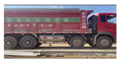 |
| 3 | 21.8 | Three-axis |  |
| 4 | 57.1 | Three-axis |  |
| 5 | 66.9 | Three-axis |  |
| 6 | 67.9 | Three-axis |  |
| 7 | 72.1 | Three-axis |  |
| 8 | 73.8 | Three-axis |  |
| 9 | 75.7 | Three-axis |  |
| 10 | 75.8 | Three-axis |  |
| Technology | Cost and Scalability | Ease of Installation and Maintenance | Anti-Electromagnetic Interference Capability | Theoretical Accuracy and Functionality Richness |
|---|---|---|---|---|
| Piezoelectric | High: sensors and backend devices are expensive. | Low: high requirements for the installation process, requiring regular calibration or replacement. | Medium, temperature sensitive | High, high weighing accuracy, but other functions are limited |
| Fiber Optic | Extremely high: both the sensors and the demodulation equipment are very expensive. | Moderate in quality, with high installation requirements, but the sensor itself is stable. | Extremely high, fully immune to electromagnetic interference | High, high precision, but cost-limiting applications |
| Inductive Loop | Low: mature technology, low cost. | Low: installation damages the pavement, easily damaged under stress. | Low, highly susceptible to interference from electromagnetic sources | Low, only capable of detecting the presence of vehicles, with limited functionality, and at risk of missing detections |
| Methods of this study (MEMS + EMD-STE) | Low cost: MEMS sensors are suitable for large-scale deployment. | High: embedded installation, low disturbance, high reliability of solid-state equipment. | High, designed to effectively resist interference | High, capable of obtaining tri-axis dynamic data, with rich features and great potential for axle-type identification |
Disclaimer/Publisher’s Note: The statements, opinions and data contained in all publications are solely those of the individual author(s) and contributor(s) and not of MDPI and/or the editor(s). MDPI and/or the editor(s) disclaim responsibility for any injury to people or property resulting from any ideas, methods, instructions or products referred to in the content. |
© 2025 by the authors. Licensee MDPI, Basel, Switzerland. This article is an open access article distributed under the terms and conditions of the Creative Commons Attribution (CC BY) license (https://creativecommons.org/licenses/by/4.0/).
Share and Cite
Li, P.; Wang, L.; Yang, S.; Ye, Z. Research on Three-Axis Vibration Characteristics and Vehicle Axle Shape Identification of Cement Pavement Under Heavy Vehicle Loads Based on EMD–Energy Decoupling Method. Sensors 2025, 25, 4066. https://doi.org/10.3390/s25134066
Li P, Wang L, Yang S, Ye Z. Research on Three-Axis Vibration Characteristics and Vehicle Axle Shape Identification of Cement Pavement Under Heavy Vehicle Loads Based on EMD–Energy Decoupling Method. Sensors. 2025; 25(13):4066. https://doi.org/10.3390/s25134066
Chicago/Turabian StyleLi, Pengpeng, Linbing Wang, Songli Yang, and Zhoujing Ye. 2025. "Research on Three-Axis Vibration Characteristics and Vehicle Axle Shape Identification of Cement Pavement Under Heavy Vehicle Loads Based on EMD–Energy Decoupling Method" Sensors 25, no. 13: 4066. https://doi.org/10.3390/s25134066
APA StyleLi, P., Wang, L., Yang, S., & Ye, Z. (2025). Research on Three-Axis Vibration Characteristics and Vehicle Axle Shape Identification of Cement Pavement Under Heavy Vehicle Loads Based on EMD–Energy Decoupling Method. Sensors, 25(13), 4066. https://doi.org/10.3390/s25134066