

Driving Pattern Analysis, Gear Shift Classification, and Fuel Efficiency in Light-Duty Vehicles: A Machine Learning Approach Using GPS and OBD II PID Signals


Abstract
1. Introduction
2. Materials and Methods
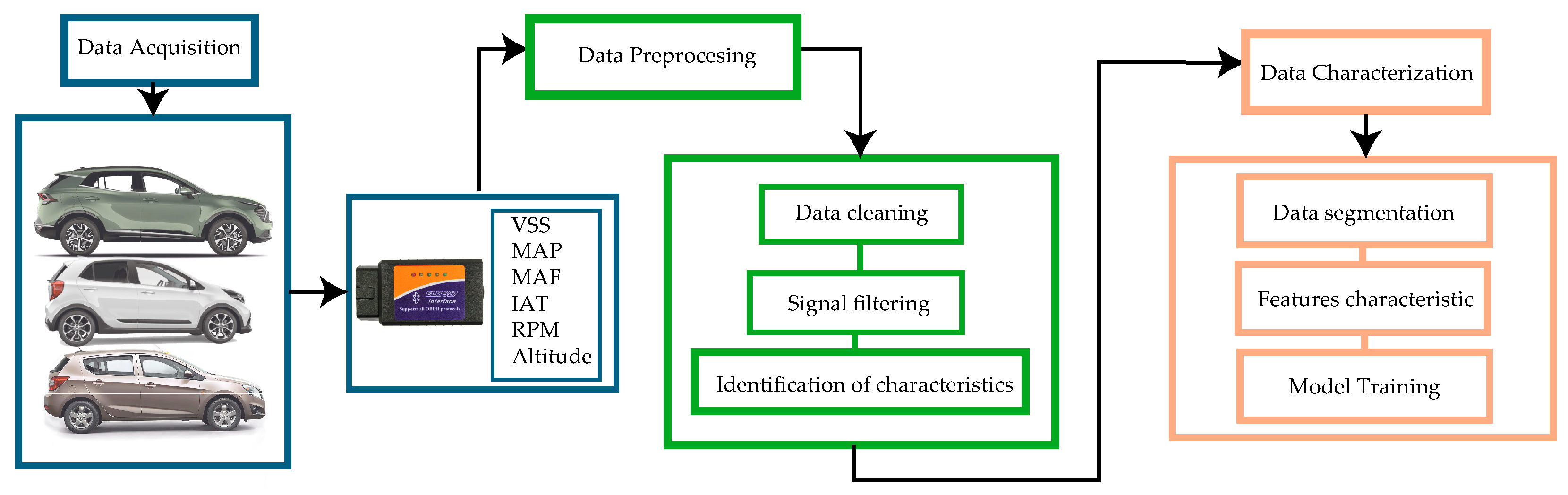
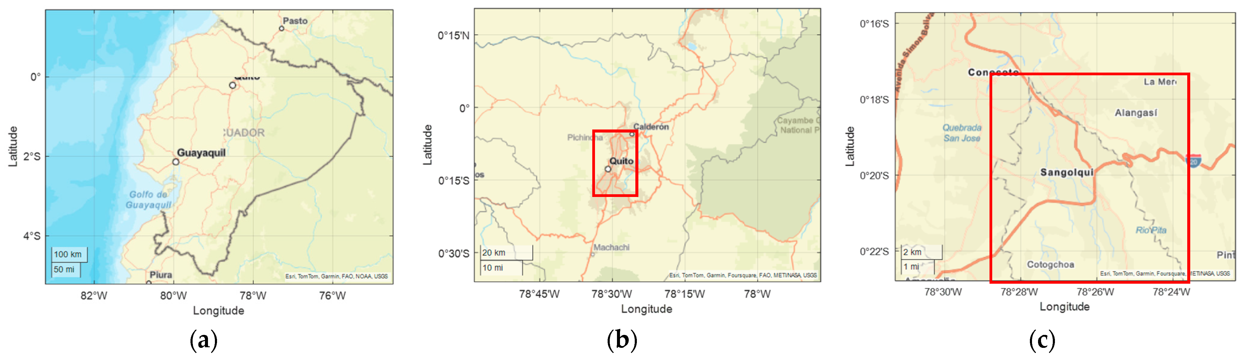
2.1. Data Collection and Analysis
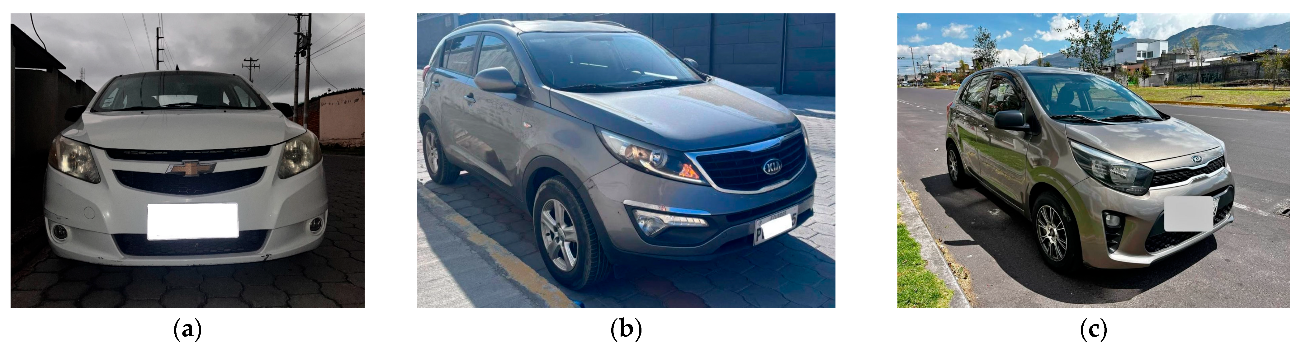
2.2. Category of M1 Vehicles
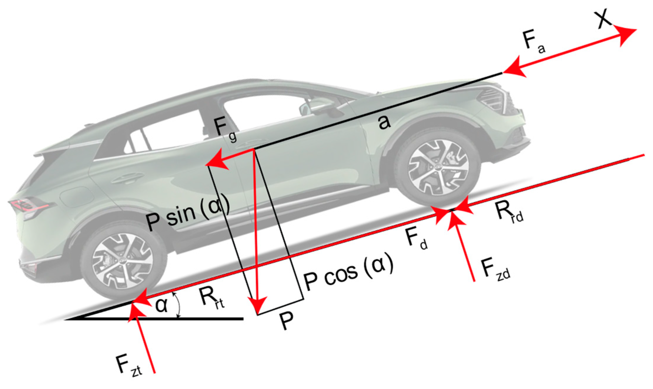
2.3. Longitudinal Vehicle Dynamics
- T = torque [Nm];
- Ft = wheel force [N];
- rn = effective radius [m].
3. Results
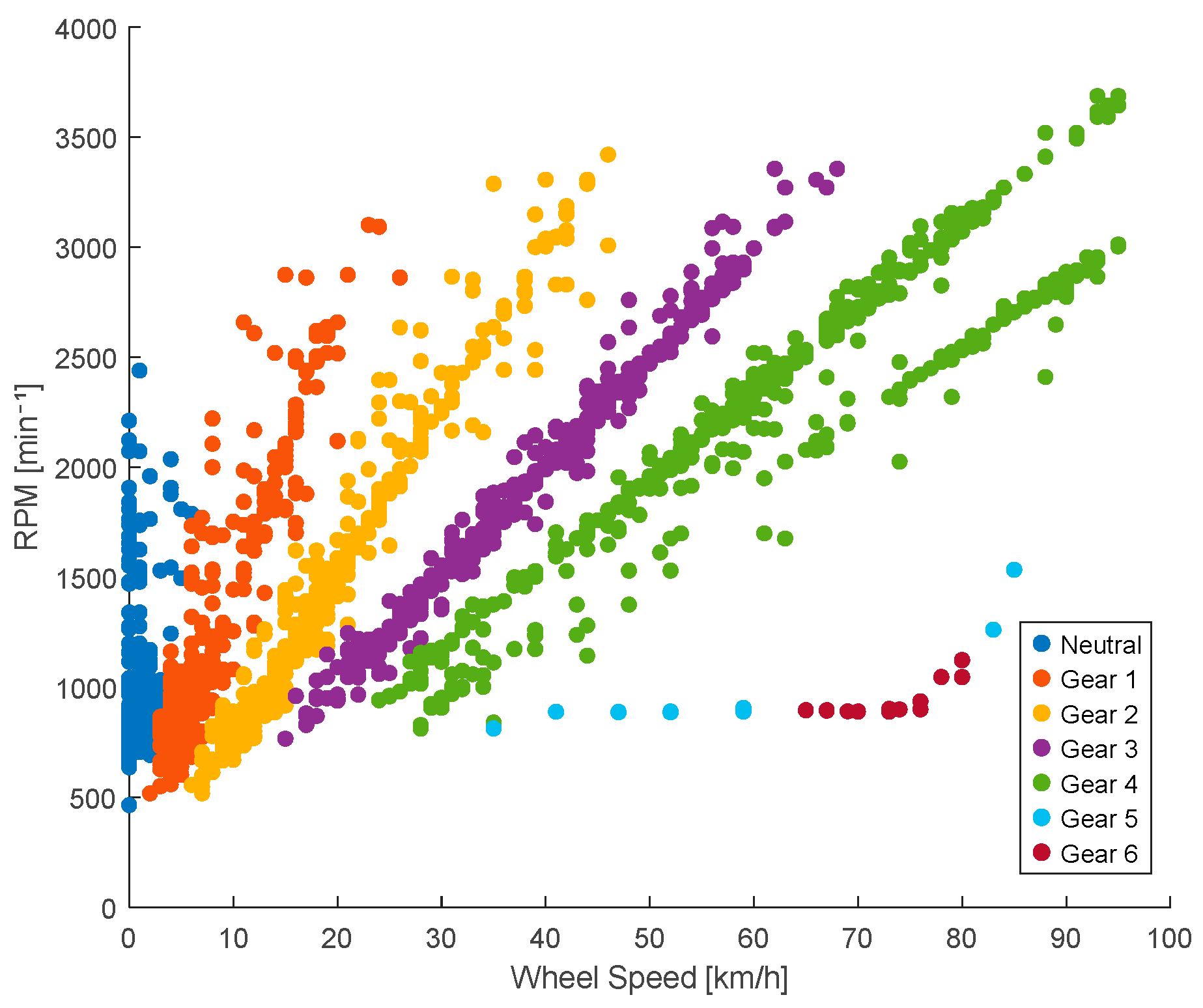
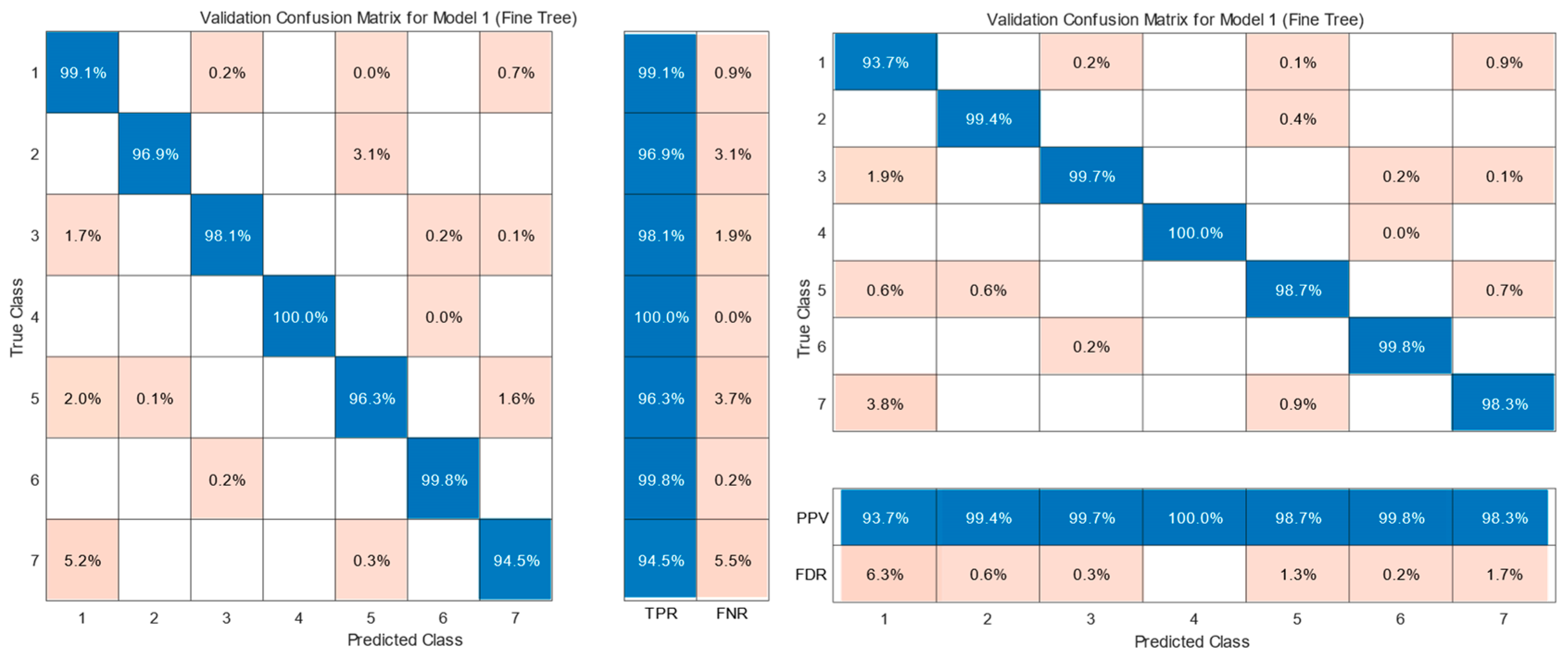
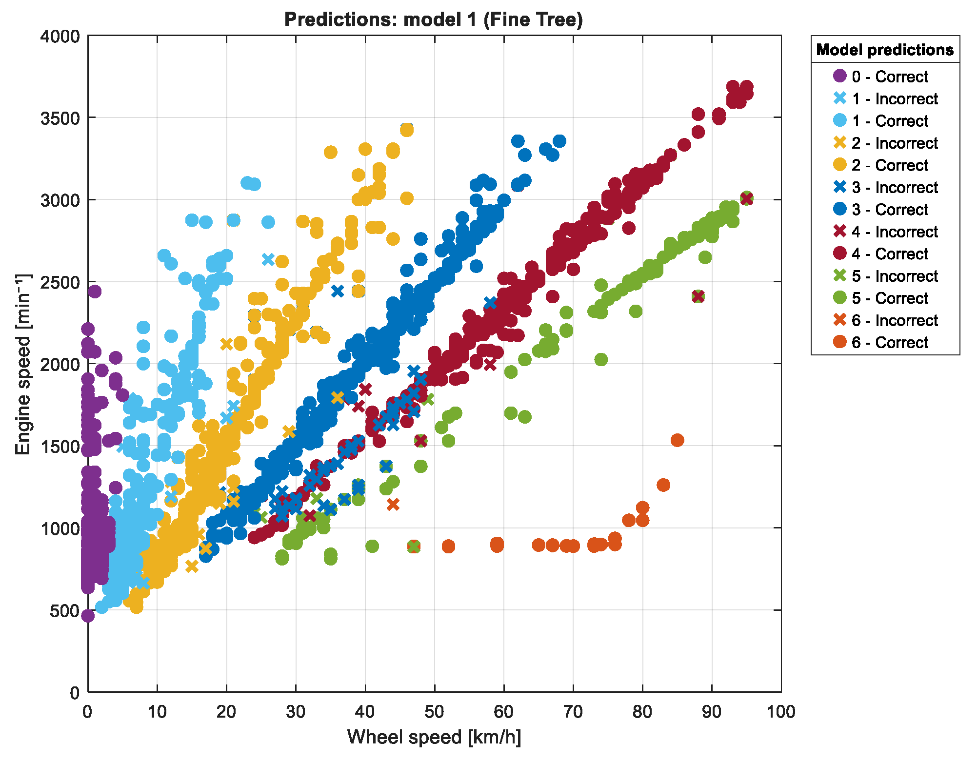
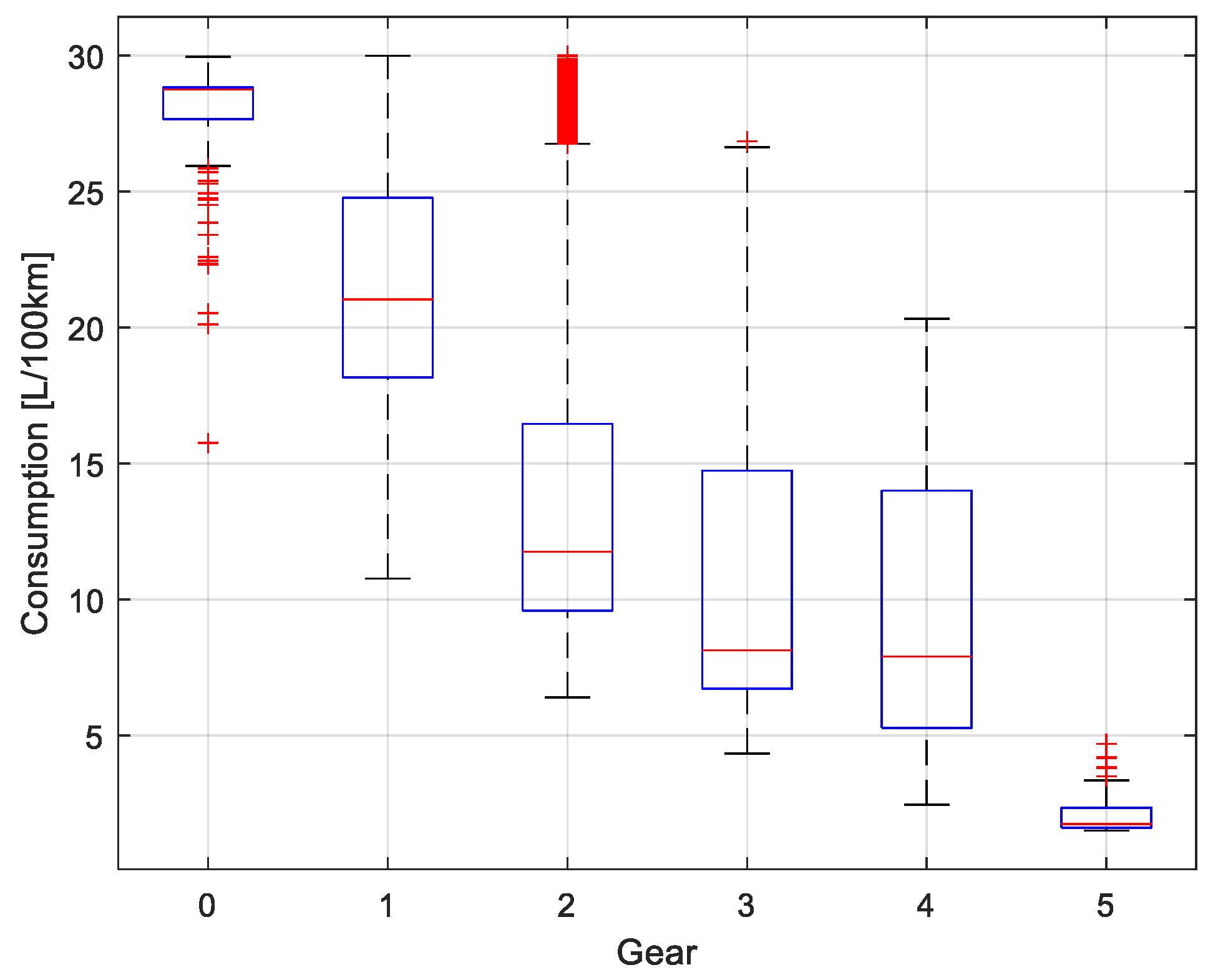
3.1. Estimation of the Performance of the Selected Gear
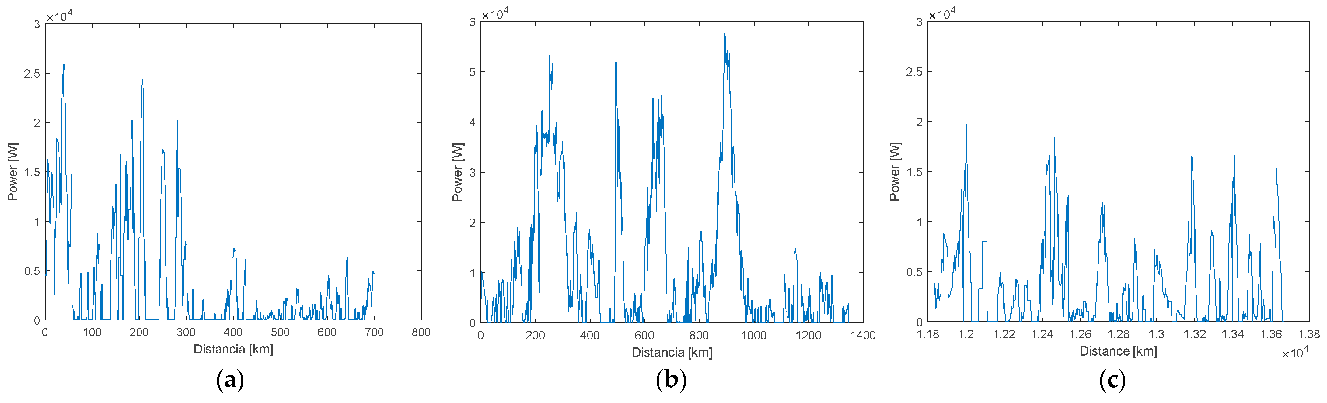
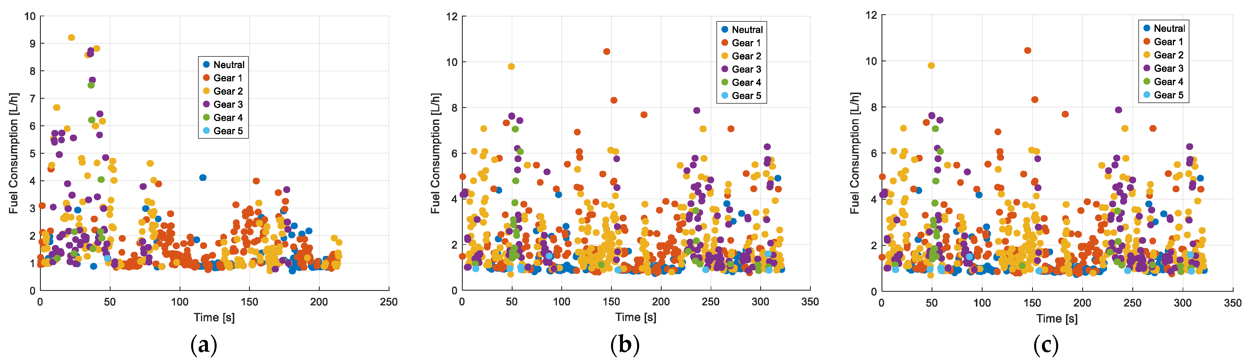
3.2. Calculating Fuel Consumption
- V = cylinder volume [cm3];
- ṁ = air mass flow [kg/s];
- RPM = engine speed.
- ARF = air–fuel ratio [dimensionless];
- = fuel density [kg/m3];
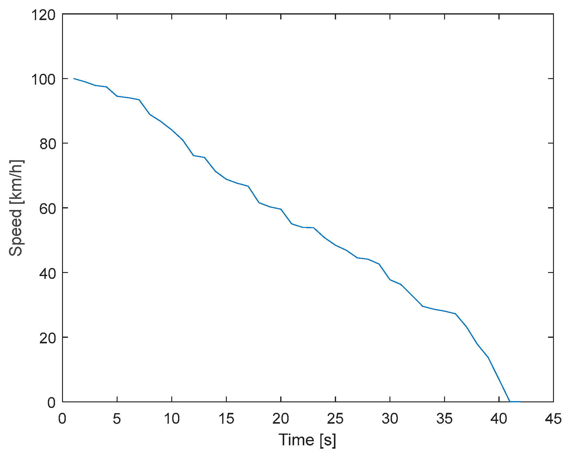
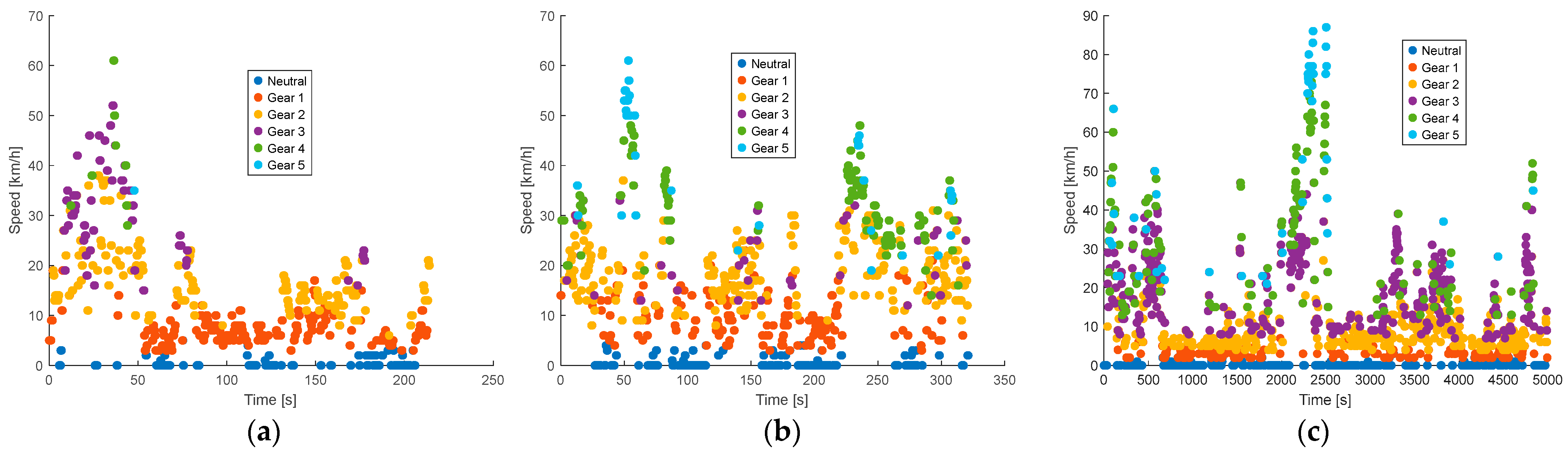
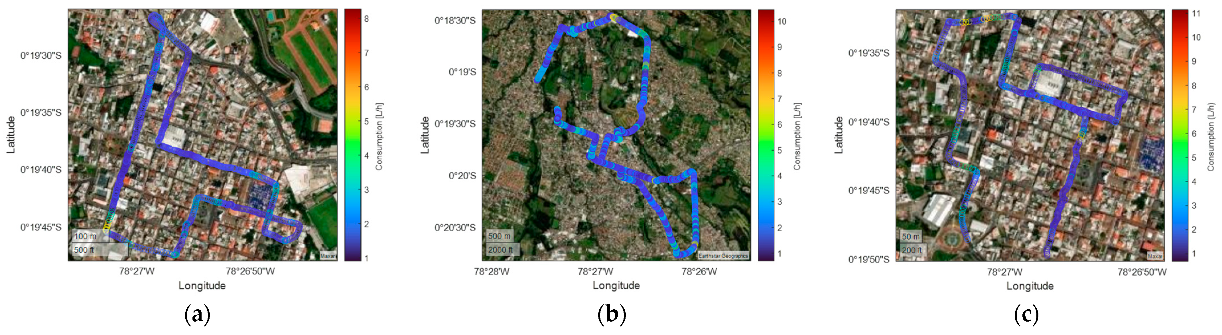
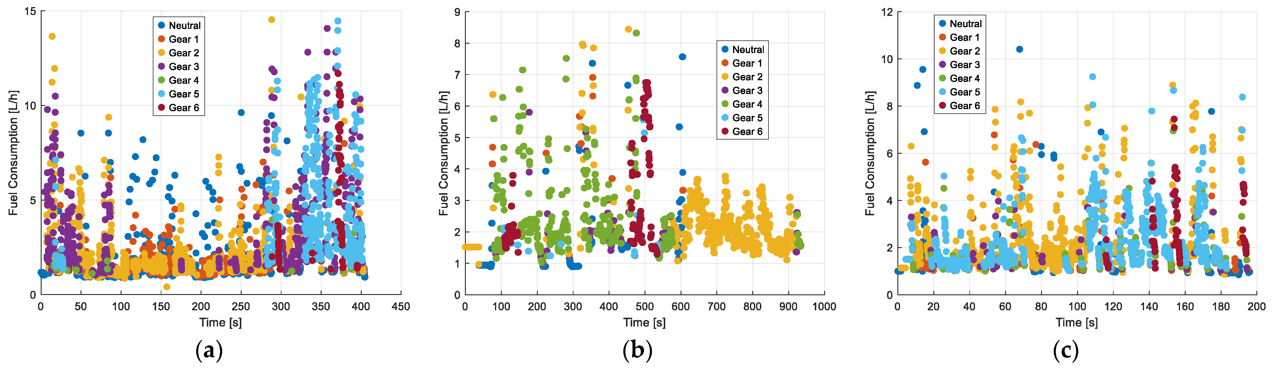
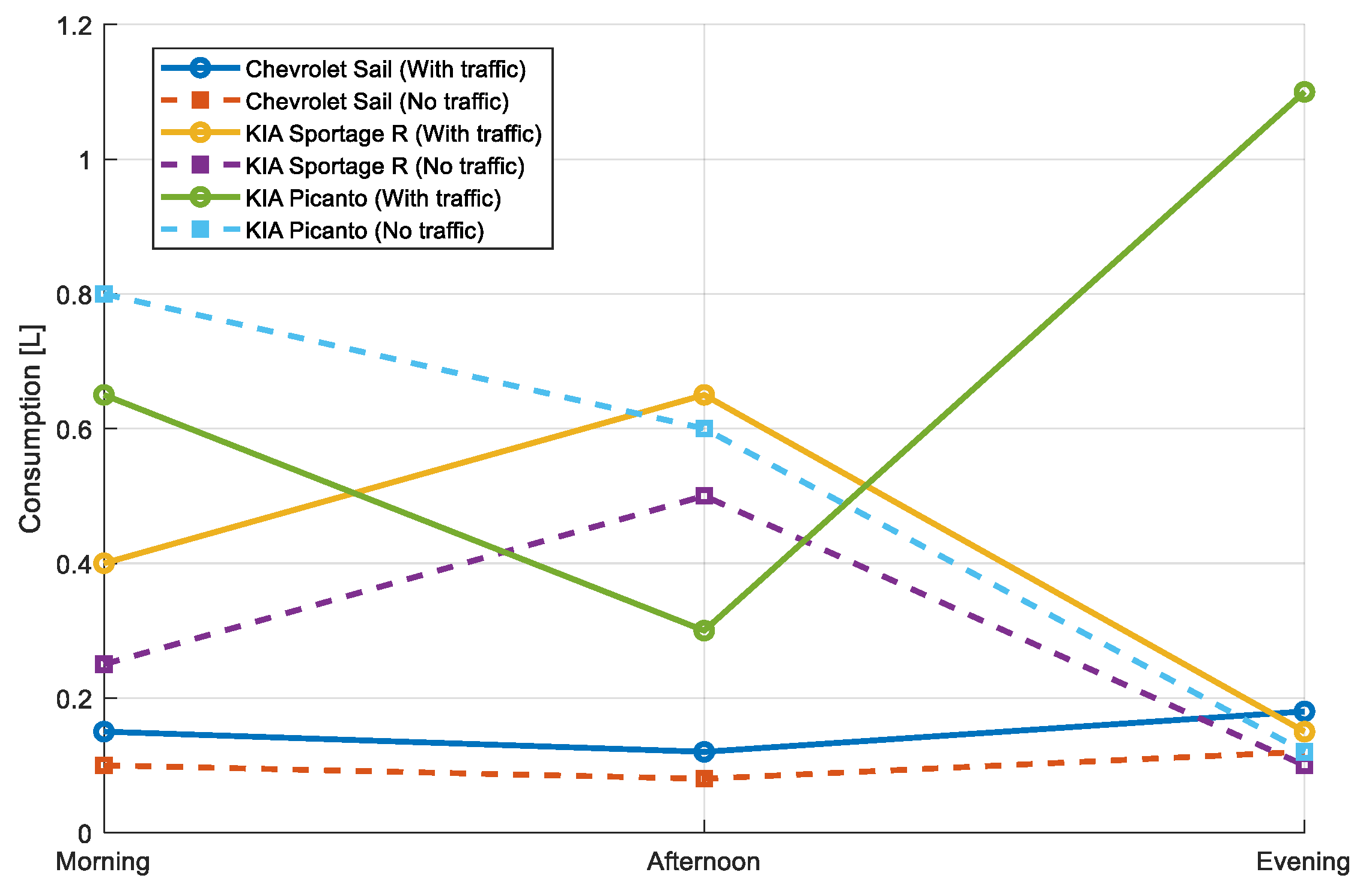
3.3. Consumption and Speed as a Function of Driving in Traffic
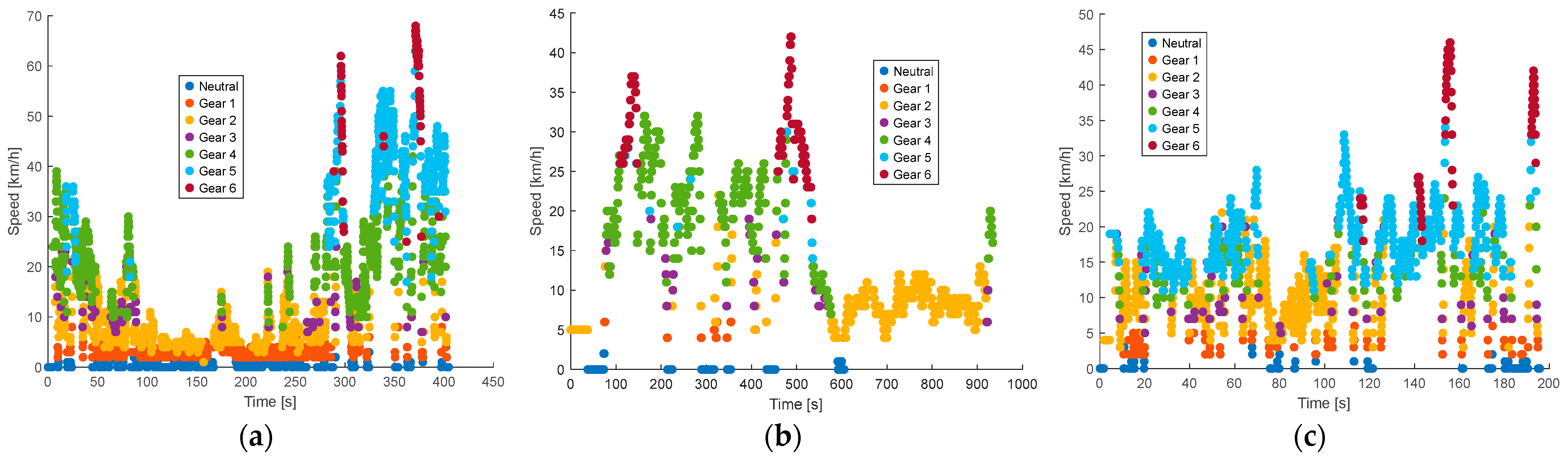
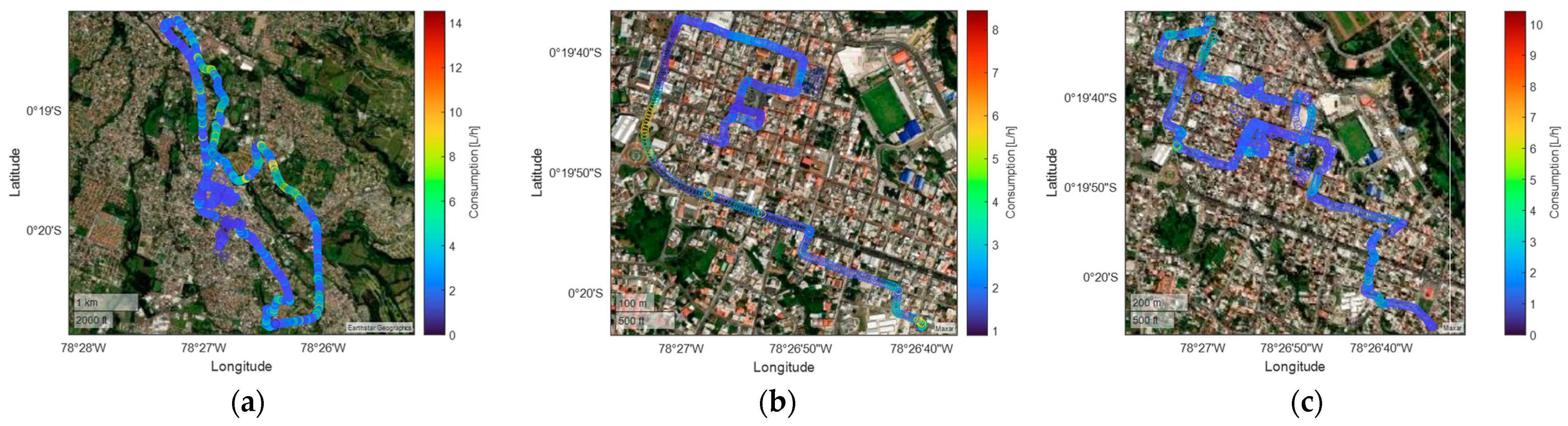
3.4. Fuel Efficiency and Speed in Gears with No Traffic
3.5. Regression Model for Instantaneous Fuel Consumption Estimation
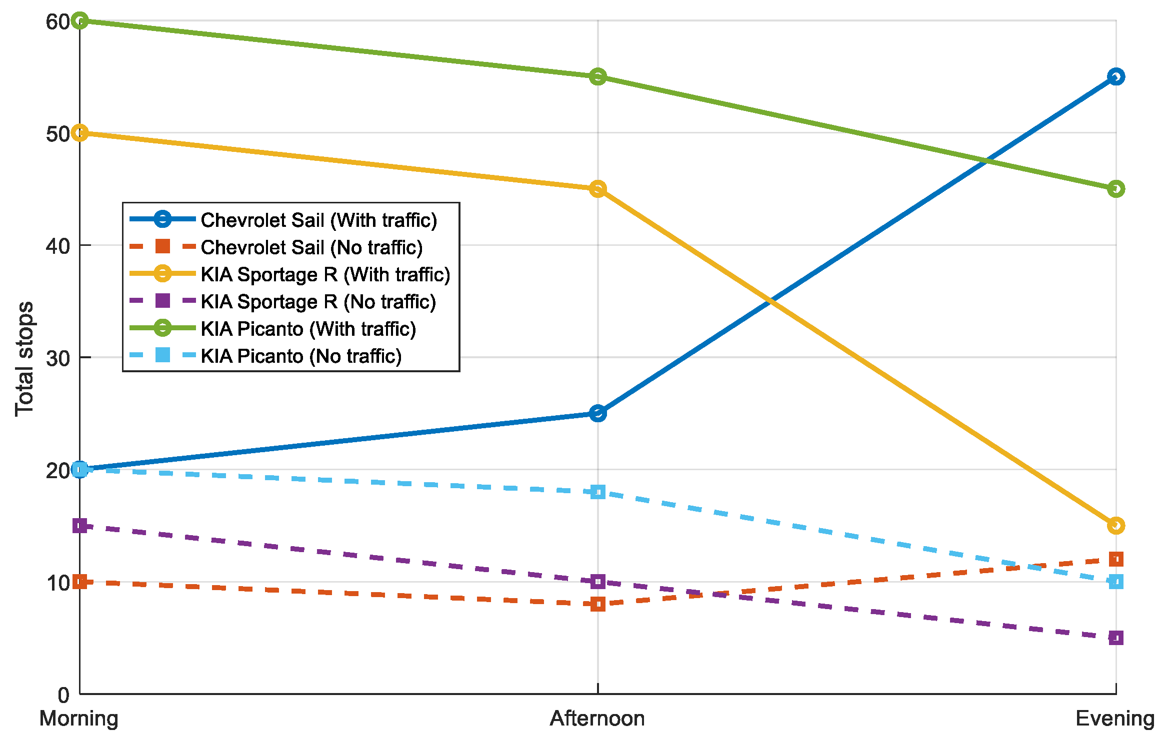
3.6. Evaluation of Fuel Consumption and Stopping Time Under Different Conditions: With and Without Traffic
4. Discussion
5. Conclusions
Author Contributions
Funding
Institutional Review Board Statement
Informed Consent Statement
Data Availability Statement
Conflicts of Interest
Abbreviations
| Af | Front area |
| Alt | Altitude |
| ANN | Artificial neural network |
| ax | Longitudinal acceleration |
| CX | Drag coefficient |
| Density | |
| Fa | Aerodynamic resistance |
| Fg | Gravitational resistance |
| Fr | Rolling resistance force |
| Fslope | Force slope |
| GPS | Global position system |
| IAT | Air intake temperature |
| Lat | Latitude |
| Lon | Longitude |
| m.a.s.l | Meters above sea level |
| m | Mass |
| OBD | On-board diagnostics |
| PID | Parameter of identification |
| P | Power |
| RDE | Real driving emissions |
| RPM | Engine speed |
| T | Torque |
| V | Volume |
References
- Al-Turki, M.; Jamal, A.; Al-Ahmadi, H.M.; Al-Sughaiyer, M.A.; Zahid, M. On the Potential Impacts of Smart Traffic Control for Delay, Fuel Energy Consumption, and Emissions: An NSGA-II-Based Optimization Case Study from Dhahran, Saudi Arabia. Sustainability 2020, 12, 7394. [Google Scholar] [CrossRef]
- Song, H.; Du, Q.; Ren, P.; Li, W.; Mehmood, A. Cloud Computing for Transportation Cyber-Physical Systems. In Cyber-Physical Systems: A Computational Perspective; Chapman Hall: London, UK, 2015. [Google Scholar]
- Aeri, M.; Purohit, K.C. Navigating the Landscape: A Comprehensive Review of State-of-the-Art Traffic Detection Approaches and Unveiling Open Research Challenges. In Proceedings of the 2024 International Conference on Electrical, Electronics and Computing Technologies, ICEECT 2024, Greater Noida, India, 29–31 August 2024; Institute of Electrical and Electronics Engineers Inc.: Piscataway, NJ, USA, 2024. [Google Scholar]
- Ghorpade, S.N.; Zennaro, M.; Chaudhari, B.S.; Ghorpade, S.N.; Zennaro, M.; Chaudhari, B.S. Node Localization for Smart Parking Systems. In Optimal Localization of Internet of Things Nodes; Springer International Publishing: Cham, Switzerland, 2022; pp. 51–66. ISBN 978-3-030-88095-8. [Google Scholar]
- Amer, H.; Salman, N.; Hawes, M.; Chaqfeh, M.; Mihaylova, L.; Mayfield, M. An Improved Simulated Annealing Technique for Enhanced Mobility in Smart Cities. Sensors 2016, 16, 1013. [Google Scholar] [CrossRef] [PubMed]
- Singh, E.; Singh, D.P. Decongesting Urban Roads: An Investigation into Causes and Challenges. In Proceedings of the Advances in Water Resources and Transportation Engineering; Mehta, Y.A., Carnacina, I., Kumar, D.N., Rao, K.R., Kumari, M., Eds.; Springer: Singapore, 2021; pp. 95–112. [Google Scholar]
- Hidalgo, D.; Huizenga, C. Implementation of Sustainable Urban Transport in Latin America. Res. Transp. Econ. 2013, 40, 66–77. [Google Scholar] [CrossRef]
- Vasconcelos Pais, F.; Nogueira, B.; Pinheiro, R.G.S. Performance Evaluation of Urban Traffic Using Simulation: A Case Study in Brazil. IEEE Lat. Am. Trans. 2023, 21, 1275–1281. [Google Scholar] [CrossRef]
- Urban Population (% of Total Population)—Ecuador. Available online: https://data.worldbank.org/indicator/SP.URB.TOTL.IN.ZS?locations=EC (accessed on 4 June 2025).
- Al-Ahmadi, H.M.; Jamal, A.; Al-Ofi, K.A.; Zahid, M.; Chen, Y. Adopting Machine Learning and Spatial Analysis Techniques for Driver Risk Assessment: Insights from a Case Study. Int. J. Environ. Res. Public Health 2020, 17, 5193. [Google Scholar] [CrossRef]
- Huang, Y.; Sun, D.; Zhang, L.H. Effects of Congestion on Drivers’ Speed Choice: Assessing the Mediating Role of State Aggressiveness Based on Taxi Floating Car Data. Accid. Anal. Prev. 2018, 117, 318–327. [Google Scholar] [CrossRef]
- Molina Campoverde, P.; Molina Campoverde, J.; Bermeo Naula, K.; Novillo, G. Efficiency Increase of Supercharged Engines. In Proceedings of the International Conference on Science, Technology and Innovation for Society, Guayaquil, Ecuador, 26–28 July 2023; Springer: Cham, Switzerland, 2023; Volume 607, pp. 346–356. [Google Scholar] [CrossRef]
- Fafoutellis, P.; Mantouka, E.G.; Vlahogianni, E.I. Eco-Driving and Its Impacts on Fuel Efficiency: An Overview of Technologies and Data-Driven Methods. Sustainability 2020, 13, 226. [Google Scholar] [CrossRef]
- Boggio-Marzet, A.; Monzon, A.; Rodriguez-Alloza, A.M.; Wang, Y. Combined Influence of Traffic Conditions, Driving Behavior, and Type of Road on Fuel Consumption. Real Driving Data from Madrid Area. Int. J. Sustain. Transp. 2022, 16, 301–313. [Google Scholar] [CrossRef]
- Ping, P.; Qin, W.; Xu, Y.; Miyajima, C.; Takeda, K. Impact of Driver Behavior on Fuel Consumption: Classification, Evaluation and Prediction Using Machine Learning. IEEE Access 2019, 7, 78515–78532. [Google Scholar] [CrossRef]
- Ma, Y.; Wang, J. Personalized Driving Behaviors and Fuel Economy over Realistic Commute Traffic: Modeling, Correlation, and Prediction. IEEE Trans. Veh. Technol. 2022, 71, 7084–7094. [Google Scholar] [CrossRef]
- Samaras, C.; Tsokolis, D.; Toffolo, S.; Magra, G.; Ntziachristos, L.; Samaras, Z. Improving Fuel Consumption and CO2 Emissions Calculations in Urban Areas by Coupling a Dynamic Micro Traffic Model with an Instantaneous Emissions Model. Transp. Res. D Transp. Environ. 2018, 65, 772–783. [Google Scholar] [CrossRef]
- Rodríguez, R.A.; Virguez, E.A.; Rodríguez, P.A.; Behrentz, E. Influence of Driving Patterns on Vehicle Emissions: A Case Study for Latin American Cities. Transp. Res. D Transp. Environ. 2016, 43, 192–206. [Google Scholar] [CrossRef]
- Hemmerle, P.; Koller, M.; Rehborn, H.; Hermanns, G.; Kerner, B.S.; Schreckenberg, M. Increased Consumption in Oversaturated City Traffic Based on Empirical Vehicle Data. In Advanced Microsystems for Automotive Applications 2014; Fischer-Wolfarth, J., Meyer, G., Eds.; Springer International Publishing: Cham, Switzerland, 2014; pp. 71–79. [Google Scholar]
- Liang, X.; Song, H.; Wu, G.; Guo, Y.; Zhang, S. Complex Traffic Flow Model for Analysis and Optimization of Fuel Consumption and Emissions at Large Roundabouts. Sustainability 2024, 16, 9464. [Google Scholar] [CrossRef]
- Falcocchio, J.C.; Levinson, H.S. The Costs and Other Consequences of Traffic Congestion. In Springer Tracts on Transportation and Traffic; Springer International Publishing: Cham, Switzerland, 2015; Volume 7, pp. 159–182. [Google Scholar]
- Kabir, R.; Remias, S.M.; Waddell, J.; Zhu, D. Time-Series Fuel Consumption Prediction Assessing Delay Impacts on Energy Using Vehicular Trajectory. Transp. Res. D Transp. Environ. 2023, 117, 103678. [Google Scholar] [CrossRef]
- Abukhalil, T.; Almahafzah, H.; Alksasbeh, M.; Alqaralleh, B.A.Y. Fuel Consumption Using OBD-II and Support Vector Machine Model. J. Robot. 2020, 2020, 9450178. [Google Scholar] [CrossRef]
- DeFries, T.H.; Sabisch, M.; Kishan, S.; Posada, F.; German, J.; Bandivadekar, A. In-Use Fuel Economy and CO2 Emissions Measurement Using OBD Data on US Light-Duty Vehicles. SAE Int. J. Engines 2014, 7, 1382–1396. [Google Scholar] [CrossRef]
- Moradi, E.; Miranda-Moreno, L. Vehicular Fuel Consumption Estimation Using Real-World Measures through Cascaded Machine Learning Modeling. Transp. Res. D Transp. Environ. 2020, 88, 102576. [Google Scholar] [CrossRef]
- SCAN TOOLS Support Company ELM327 OBD-II. Available online: https://www.scantool.net/catalogsearch/result/?q=elm327 (accessed on 25 March 2025).
- Instituto Nacional de Estadística y Censos (INEC) Censo Ecuador. Available online: https://www.censoecuador.gob.ec/ (accessed on 25 March 2025).
- Servicio Ecuatoriano de Normalización (INEN) Clasificación de Vehicular NTE INEN 2656. Available online: https://www.normalizacion.gob.ec/inspeccion-de-vehiculos-automotores-bajo-reglamentos-tecnicos-inen/ (accessed on 25 March 2025).
- Molina-Campoverde, J.J.; Rivera-Campoverde, N.; Molina Campoverde, P.A.; Bermeo Naula, A.K. Urban Mobility Pattern Detection: Development of a Classification Algorithm Based on Machine Learning and GPS. Sensors 2024, 24, 3884. [Google Scholar] [CrossRef]
- Sun, Z.; Premarathna, W.A.A.S.; Anupam, K.; Kasbergen, C.; Erkens, S.M.J.G. A State-of-the-Art Review on Rolling Resistance of Asphalt Pavements and Its Environmental Impact. Constr. Build Mater. 2024, 411, 133589. [Google Scholar] [CrossRef]
- Huertas, J.I.; Andrés, G.; Coello, Á. Accuracy and Precision of the Drag and Rolling Resistance Coefficients Obtained by on Road Coast down Tests. In Proceedings of the International Conference on Industrial Engineering and Operations Management, Bogota, Colombia, 25–26 October 2017; Volume 7. Available online: https://ieomsociety.org/bogota2017/papers/97.pdf (accessed on 4 June 2025).
- Molina Campoverde, J.J. Driving Mode Estimation Model Based in Machine Learning Through PID’s Signals Analysis Obtained From OBD II. In Proceedings of the International Conference on Applied Technologies, Quito, Ecuador, 2–4 December 2020; Volume 1194, pp. 80–91. [Google Scholar] [CrossRef]
- Andrade, P.; Silva, I.; Silva, M.; Flores, T.; Cassiano, J.; Costa, D.G. A TinyML Soft-Sensor Approach for Low-Cost Detection and Monitoring of Vehicular Emissions. Sensors 2022, 22, 3838. [Google Scholar] [CrossRef]
- Campoverde, P.M.; Benavides, K.; Montenegro, F.; Molina, J. Fuel Consumption Analysis of an MPI Engine by Varying Fuel Type, Fuel Filtering, and Air Filter Employing a Full-Factor Analysis. In Proceedings of the ECTM 2023—2023 IEEE 7th Ecuador Technical Chapters Meeting, Ambato, Ecuador, 10–13 October 2023. [Google Scholar] [CrossRef]
- Molina Campoverde, J.; Molina Campoverde, P.; Rivera Campoverde, N. Fundamentos de Los Sistemas de Inyección a Gasolina y Autotrónica Automotriz. Available online: https://dspace.ups.edu.ec/handle/123456789/30396 (accessed on 4 June 2025).
- Al-refai, G.; Al-refai, M.; Alzu’bi, A. Driving Style and Traffic Prediction with Artificial Neural Networks Using On-Board Diagnostics and Smartphone Sensors. Appl. Sci. 2024, 14, 5008. [Google Scholar] [CrossRef]
- Vasavi, S.; Aswarth, K.; Sai Durga Pavan, T.; Anu Gokhale, A. Predictive Analytics as a Service for Vehicle Health Monitoring Using Edge Computing and AK-NN Algorithm. Mater. Today Proc. 2021, 46, 8645–8654. [Google Scholar] [CrossRef]
- Tollner, D.; Zöldy, M. Road Type Classification of Driving Data Using Neural Networks. Computers 2025, 14, 70. [Google Scholar] [CrossRef]


| Variables | Nomenclature | Range | Units |
|---|---|---|---|
| Vehicle Speed Sensor | VSS | 0–110 | km/h |
| Engine Speed | RPM | 0–6000 | min−1 |
| Engine Coolant Temperature | ECT | 0–92 | °C |
| Intake Air Temperature | IAT | 8–42 | °C |
| Manifold Absolute Pressure | MAP | 16–75 | kPa |
| Mass Air Flow | MAF | 0–35 | g/s |
| Throttle Position Sensor | TPS | 0–100 | % |
| Vehicle | Brand | Model | Year | Odometer [km] | Vehicle Weight [kg] | Engine Displacement [cm3] | Torque [Nm] | Power [kW] | Number of Gears |
|---|---|---|---|---|---|---|---|---|---|
| Vehicle 1 | KIA | Picanto | 2018 | 115,349 | 886 | 998 | 141@4850 rpm | 69@6300 rpm | 5 + Reverse |
| Vehicle 2 | Chevrolet | Sail | 2013 | 315,622 | 1087 | 1400 | 131@4200 rpm | 76@6000 rpm | 5 + Reverse |
| Vehicle 3 | KIA | Sportage R | 2020 | 98,458 | 1490 | 2000 | 191@4700 rpm | 112@6200 rpm | 6 + Reverse |
| Route | Vehicle | Date | Start Time | End Time |
|---|---|---|---|---|
| Vehicle 1 | Chevrolet Sail | Tuesday 05/11/2024 | 13:18:52 | 14:12:24 |
| Thursday 07/11/2024 | 17:37:10 | 19:00:22 | ||
| Friday 03/01/2025 | 09:12:28 | 09:48:12 | ||
| Vehicle 2 | KIA Sportage R | Monday 30/12/2024 | 09:32:26 | 10:13:23 |
| Monday 30/12/204 | 13:48:44 | 14:48:13 | ||
| Monday 30/12/2024 | 17:50:11 | 19:12:57 | ||
| Vehicle 3 | KIA Picanto | Friday 15/11/2024 | 13:39:26 | 14:17:14 |
| Friday 03/12/2024 | 08:48:04 | 10:08:36 | ||
| Monday 30/12/2024 | 18:58:08 | 19:34:21 |
| Route | Vehicle | Date | Start Time | End Time |
|---|---|---|---|---|
| Vehicle 1 | Chevrolet Sail | Monday 10/02/2025 | 11:03:59 | 11:27:18 |
| Friday 28/02/2025 | 13:42:43 | 14:19:20 | ||
| Friday 28/02/2025 | 16:37:23 | 17:10:06 | ||
| Vehicle 2 | KIA Sportage R | Monday 17/02/2025 | 15:52:16 | 16:07:51 |
| Wednesday 26/02/2025 | 19:35:00 | 20:07:38 | ||
| Thursday 27/02/2025 | 10:35:13 | 11:42:40 | ||
| Vehicle 3 | KIA Picanto | Monday 03/03/2025 | 20:11:35 | 20:25:37 |
| Wednesday 05/03/2025 | 15:32:41 | 15:58:21 | ||
| Friday 07/03/2025 | 09:54:22 | 10:21:57 |
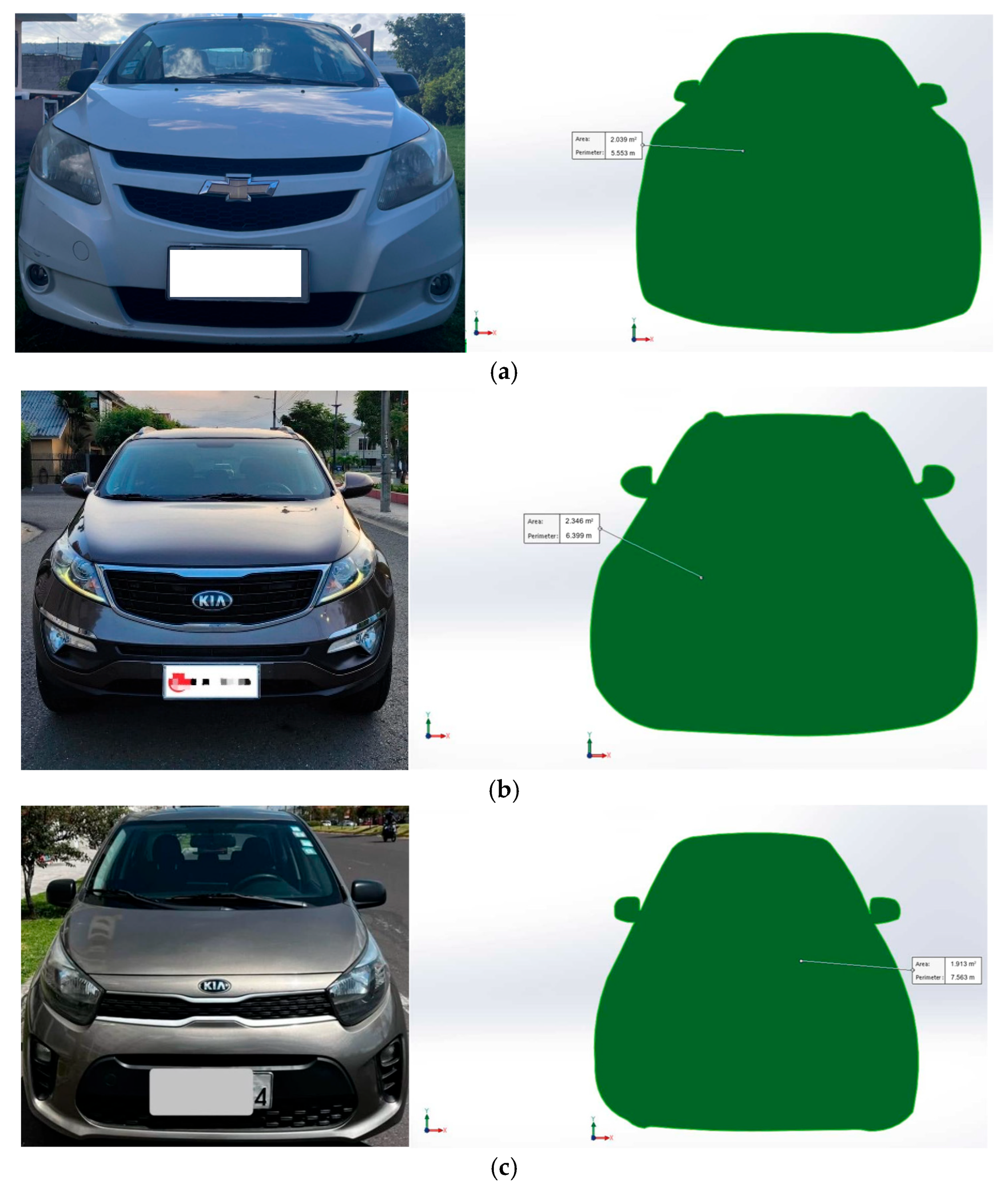
| Vehicle | Brand | Model | Height [mm] | Width [mm] | Frontal Area [mm2] | Frontal Area [m2] |
|---|---|---|---|---|---|---|
| Vehicle 1 | KIA | Picanto | 1595 | 1495 | 1,912,864.54 | 1.913 |
| Vehicle 2 | Chevrolet | Sail | 1503 | 1690 | 2,039,072.22 | 2.039 |
| Vehicle 3 | KIA | Sportage R | 1645 | 1855 | 2,346,431.97 | 2.346 |
| Model | Accuracy Validation (%) | Error Rate Validation (%) | Precision Avg (%) | Recall Avg (%) | F1-Score Avg (%) | Training Time (s) | Prediction Speed (obs/s) |
|---|---|---|---|---|---|---|---|
| 1 Tree (Fine Tree) | 98.5 | 1.5 | 98.6 | 98.5 | 98.5 | 15.340 | ~85,000 |
| 2 Tree (Medium Tree) | 86.8 | 13.2 | 87.0 | 86.8 | 86.9 | 12.890 | ~90,000 |
| 3 Tree (Coarse Tree) | 70.7 | 29.3 | 71.0 | 70.7 | 70.8 | 10.560 | ~95,000 |
| 4 KNN (Fine KNN) | 99.7 | 0.3 | 99.8 | 99.7 | 99.8 | 27.245 | ~78,000 |
| 5 KNN (Medium KNN) | 98.1 | 1.9 | 98.2 | 98.1 | 98.1 | 25.780 | ~76,000 |
| 6 KNN (Coarse KNN) | 87.7 | 12.3 | 87.9 | 87.7 | 87.8 | 20.450 | ~80,000 |
| 7 KNN (Cosine KNN) | 98.2 | 1.8 | 98.3 | 98.2 | 98.2 | 28.340 | ~77,000 |
| 8 KNN (Cubic KNN) | 97.9 | 2.1 | 98.0 | 97.9 | 97.9 | 29.120 | ~75,000 |
| 9 KNN(Weighted KNN) | 99.6 | 0.4 | 99.7 | 99.6 | 99.7 | 30.120 | ~75,000 |
| 10 Logistic Regression | 72.0 | 28.0 | 72.5 | 72.0 | 72.2 | 8.230 | ~100,000 |
| 11 Efficient Linear SVM | 93.7 | 6.3 | 93.8 | 93.7 | 93.7 | 18.560 | ~88,000 |
| True Class | 1 | 2 | 3 | 4 | 5 | 6 | 7 |
|---|---|---|---|---|---|---|---|
| 1 | 4150 | 0 | 6 | 1 | 0 | 0 | 2 |
| 2 | 0 | 159 | 0 | 0 | 0 | 0 | 0 |
| 3 | 1 | 0 | 5033 | 0 | 0 | 7 | 0 |
| 4 | 0 | 0 | 0 | 5303 | 0 | 15 | 0 |
| 5 | 0 | 0 | 0 | 0 | 1315 | 0 | 3 |
| 6 | 0 | 0 | 10 | 20 | 0 | 5234 | 0 |
| 7 | 10 | 0 | 0 | 0 | 1 | 0 | 3208 |
| Variable | Estimate | SE | tStat | Interpretation |
|---|---|---|---|---|
| Intercept | 20.86 | 0.17236 | 121.12 | Estimated baseline consumption when all explanatory variables are zero. |
| VSS | −0.0910 | 0.0020152 | −44.787 | For each additional 1 km/h, consumption decreases by 0.0910 L/100 km. |
| RPM | 0.00089 | 3.8004 × 10⁻⁵ | 22.957 | For each additional 1 RPM, consumption increases by 0.00089 L/100 km. |
| MAP | 0.3277 | 0.0006457 | 507.34 | For each additional 1 kPa in manifold pressure (MAP), consumption increases by 0.3277. |
| Ax | 0.1743 | 0.027113 | 6.6654 | Accelerations increase consumption by 0.1743 L/100 km per unit of measurement. |
| Gear1 | −7.6751 | 0.16822 | −45.641 | Using gear 1 reduces 7.68 L/100 km compared to the base category. |
| Gear2 | −16.33 | 0.16853 | −96.937 | Gear 2: −16.33 L/100 km compared to neutral. |
| Gear3 | −19.89 | 0.17245 | −115.44 | Gear 3: −19.89 L/100 km compared to neutral. |
| Gear4 | −22.05 | 0.18252 | −120.95 | Gear 4: −22.05 L/100 km compared to neutral. |
| Gear5 | −20.05 | 0.2575 | −79.055 | Gear 5: −20.05 L/100 km compared to neutral. |
Disclaimer/Publisher’s Note: The statements, opinions and data contained in all publications are solely those of the individual author(s) and contributor(s) and not of MDPI and/or the editor(s). MDPI and/or the editor(s) disclaim responsibility for any injury to people or property resulting from any ideas, methods, instructions or products referred to in the content. |
© 2025 by the authors. Licensee MDPI, Basel, Switzerland. This article is an open access article distributed under the terms and conditions of the Creative Commons Attribution (CC BY) license (https://creativecommons.org/licenses/by/4.0/).
Share and Cite
Molina-Campoverde, J.J.; Zurita-Jara, J.; Molina-Campoverde, P. Driving Pattern Analysis, Gear Shift Classification, and Fuel Efficiency in Light-Duty Vehicles: A Machine Learning Approach Using GPS and OBD II PID Signals. Sensors 2025, 25, 4043. https://doi.org/10.3390/s25134043
Molina-Campoverde JJ, Zurita-Jara J, Molina-Campoverde P. Driving Pattern Analysis, Gear Shift Classification, and Fuel Efficiency in Light-Duty Vehicles: A Machine Learning Approach Using GPS and OBD II PID Signals. Sensors. 2025; 25(13):4043. https://doi.org/10.3390/s25134043
Chicago/Turabian StyleMolina-Campoverde, Juan José, Juan Zurita-Jara, and Paúl Molina-Campoverde. 2025. "Driving Pattern Analysis, Gear Shift Classification, and Fuel Efficiency in Light-Duty Vehicles: A Machine Learning Approach Using GPS and OBD II PID Signals" Sensors 25, no. 13: 4043. https://doi.org/10.3390/s25134043
APA StyleMolina-Campoverde, J. J., Zurita-Jara, J., & Molina-Campoverde, P. (2025). Driving Pattern Analysis, Gear Shift Classification, and Fuel Efficiency in Light-Duty Vehicles: A Machine Learning Approach Using GPS and OBD II PID Signals. Sensors, 25(13), 4043. https://doi.org/10.3390/s25134043