
Effective Denoising of Multi-Source Partial Discharge Signals via an Improved Power Spectrum Segmentation Method Based on Normalized Spectral Kurtosis


Abstract
1. Introduction
2. Basic Theory
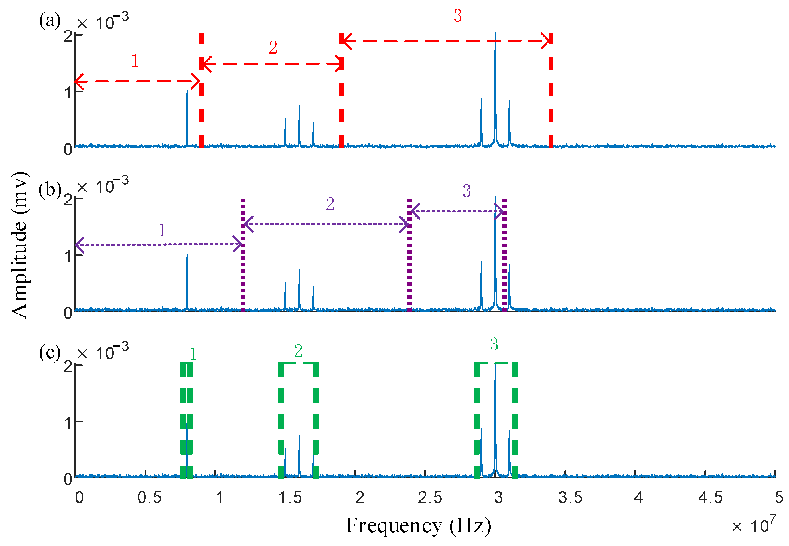
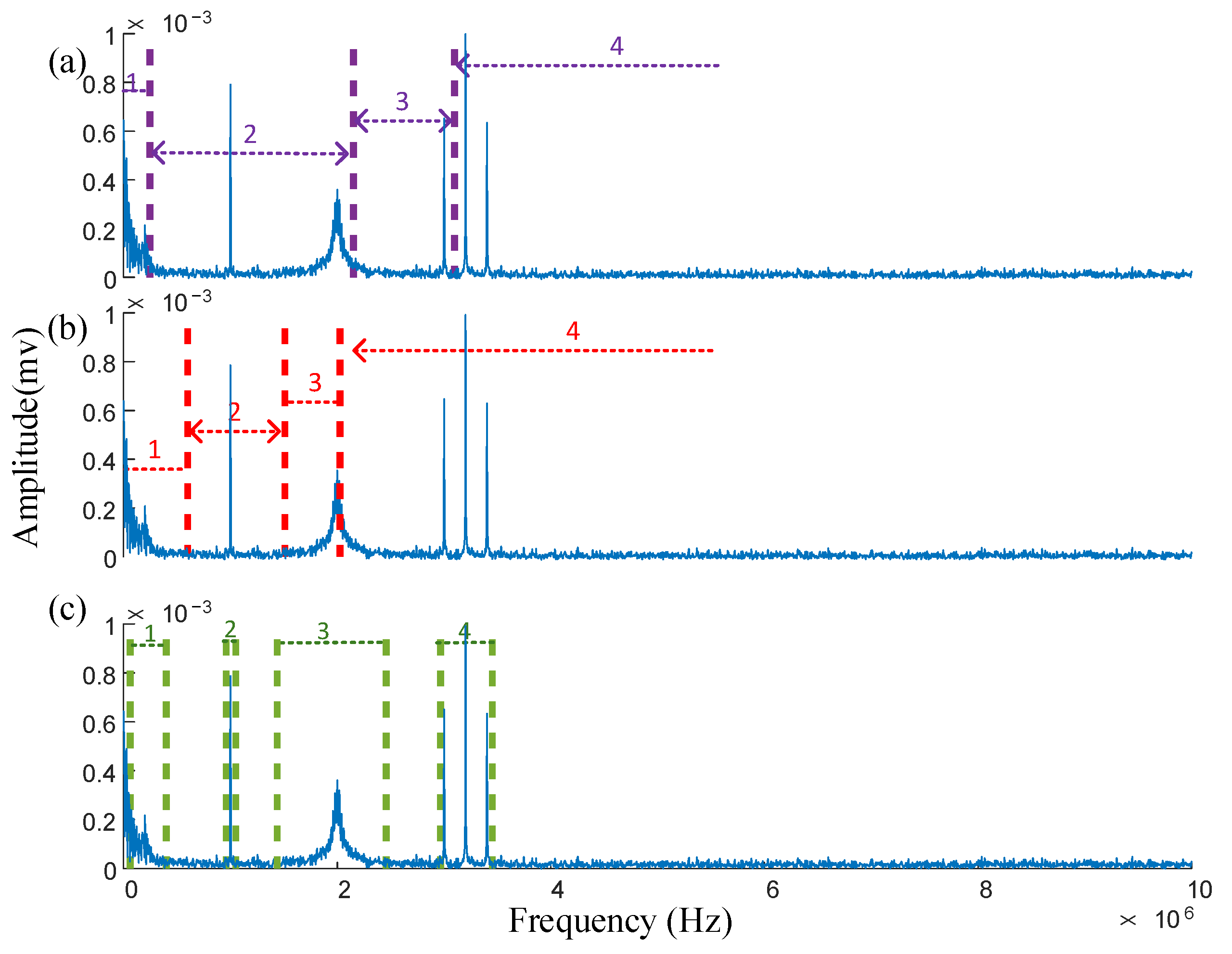
2.1. Common Spectrum Segmentation Methods
2.2. Improved Welch Power Spectrum Segmentation Methods
- (1)
- Calculate the signal segmented power spectrum: Divide the signal into L segments. If each segment overlaps by half, then , where N is the length of each segment and M is the number of overlapping points. The power spectrum of each segment is calculated aswhere is the normalization factor, is the window function, and is the i-th segment of the signal.
- (2)
- Calculate the average power spectrum :
- (3)
- Determine the center frequencies and boundary positions of each frequency band: Extract all local maxima and their positions from , and compile this information into a set , where J represents the total number of maxima in the power spectrum. Based on the distribution of the power spectrum, select the locations of the top K maxima as the center frequencies of the frequency bands. Then, determine the upper and lower sideband frequencies according to the amplitude variation relationships. The steps are as follows:
- (1)
- Determine the amplitude threshold for boundary selection:where w is the bandwidth control coefficient, determined as described in Section 2.3.
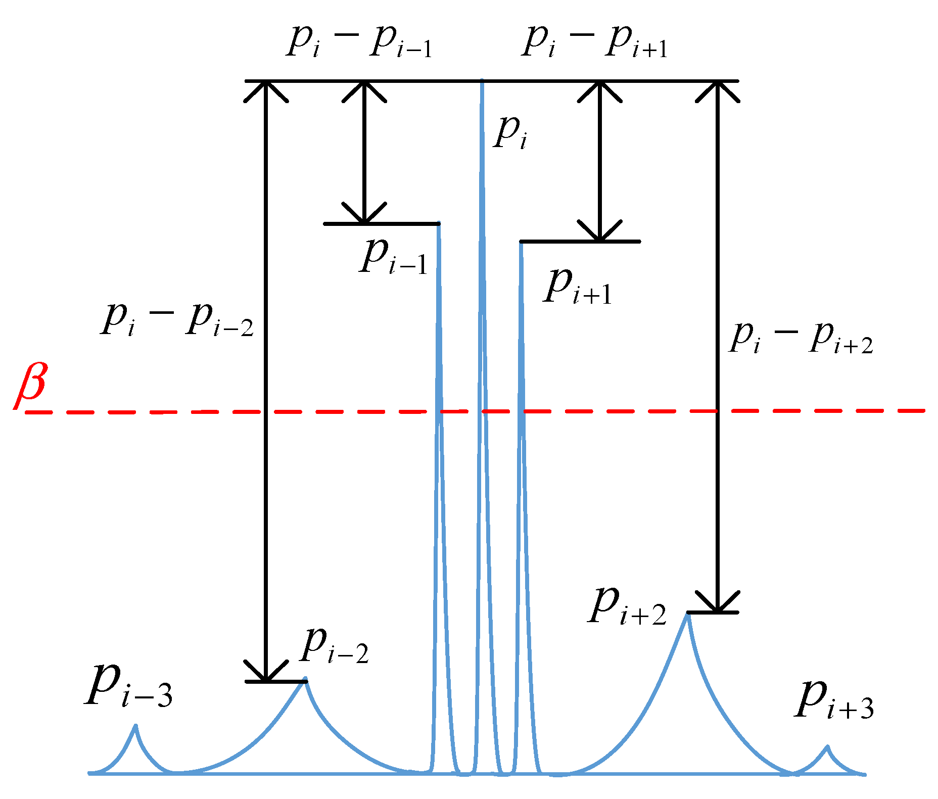
- (2)
- Determine the center frequency and boundary positions. Taking as the center, is compared with its adjacent extreme value on the right side. If , the corresponding frequency of is taken as the upper side frequency position. If the above conditions are not met, the next adjacent extreme value on the right side of is compared with the amplitude to determine whether it is greater than the threshold . Repeat this process until the condition is met. The lower boundary is determined similarly. The relationship between the center frequency amplitude and boundary amplitude is illustrated in Figure 2.
2.3. Improved Welch Power Spectrum Segmentation Methods’ Selection Based on Normalized Power Spectrum Kurtosis
- (1)
- Power spectral kurtosis calculation: The PSK for segmented signals is computed aswhere is the power spectrum value at the i-th frequency point, and is the average power spectrum value.
- (2)
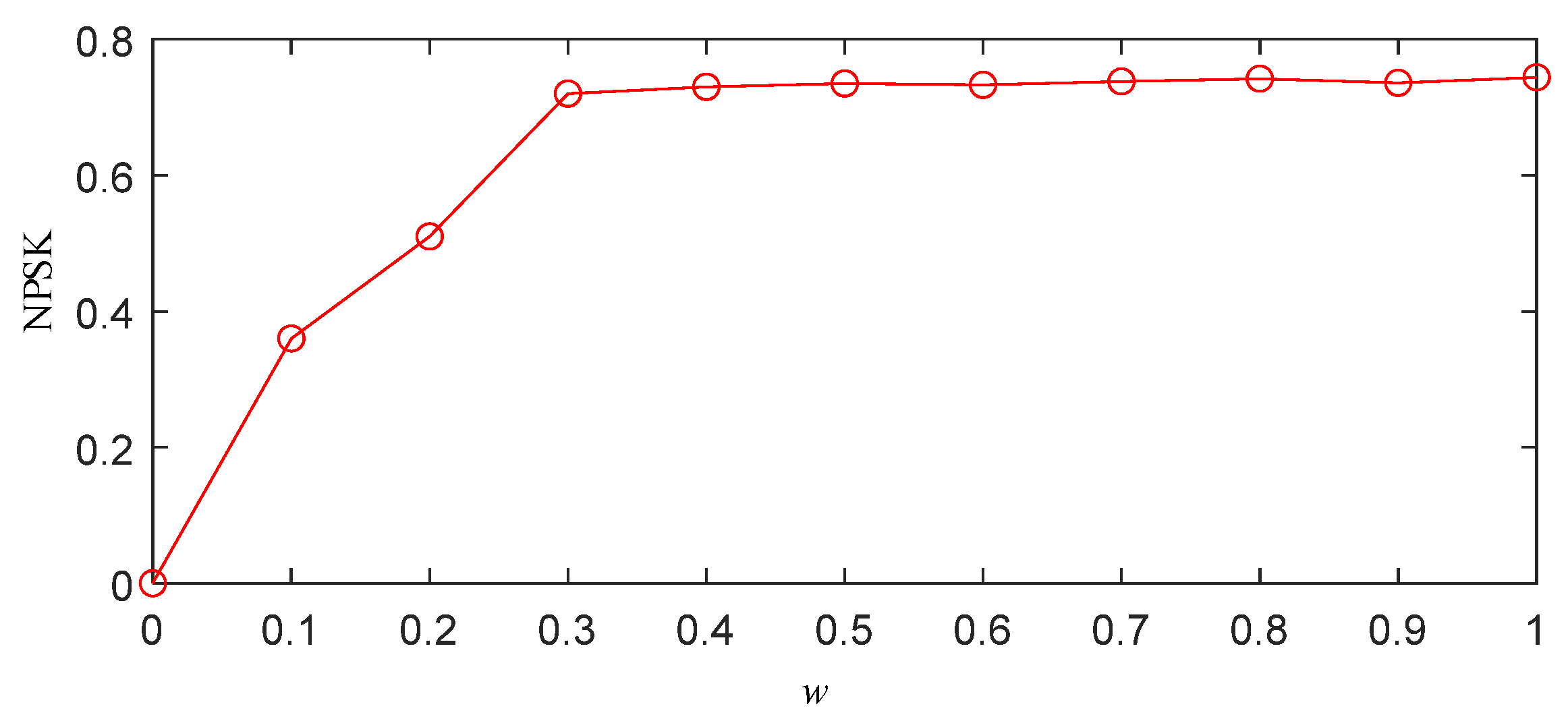
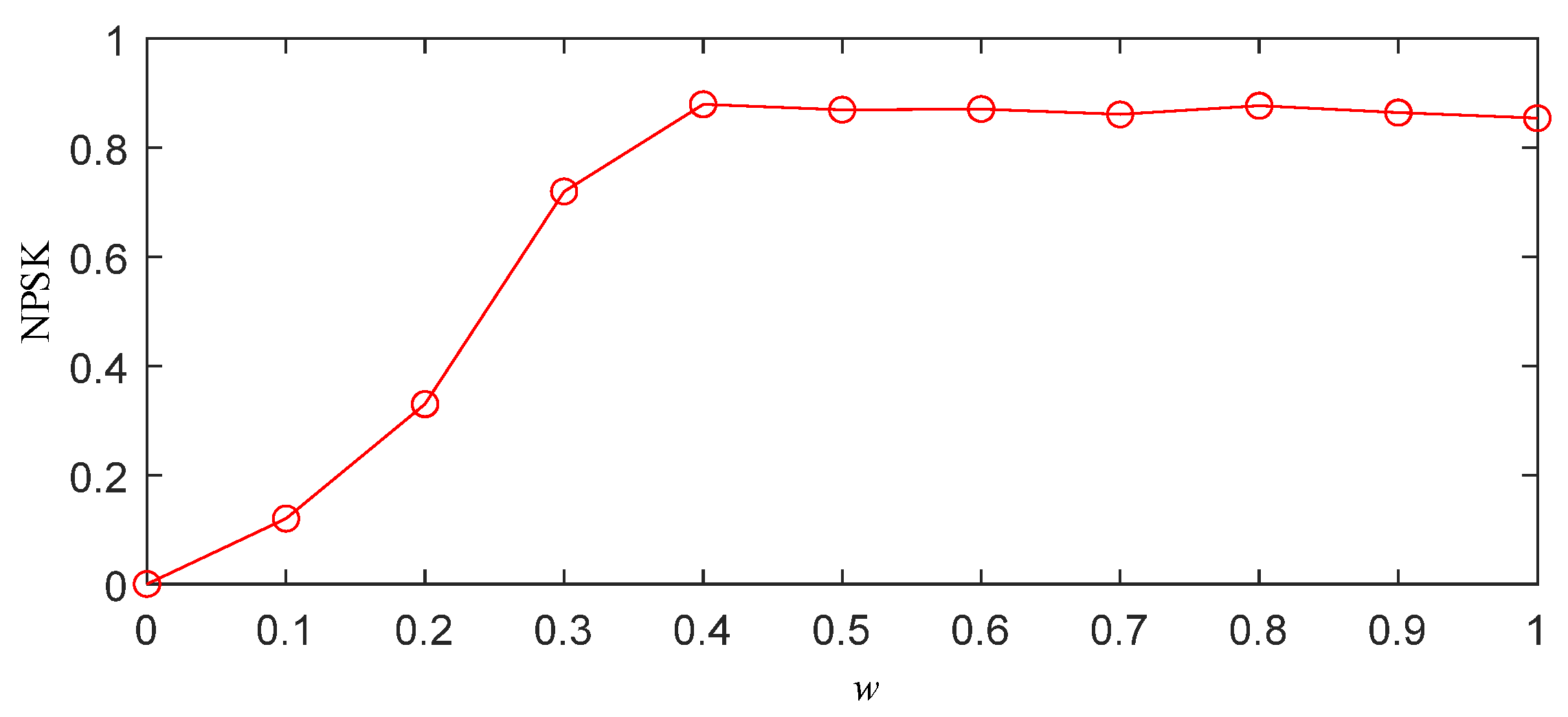
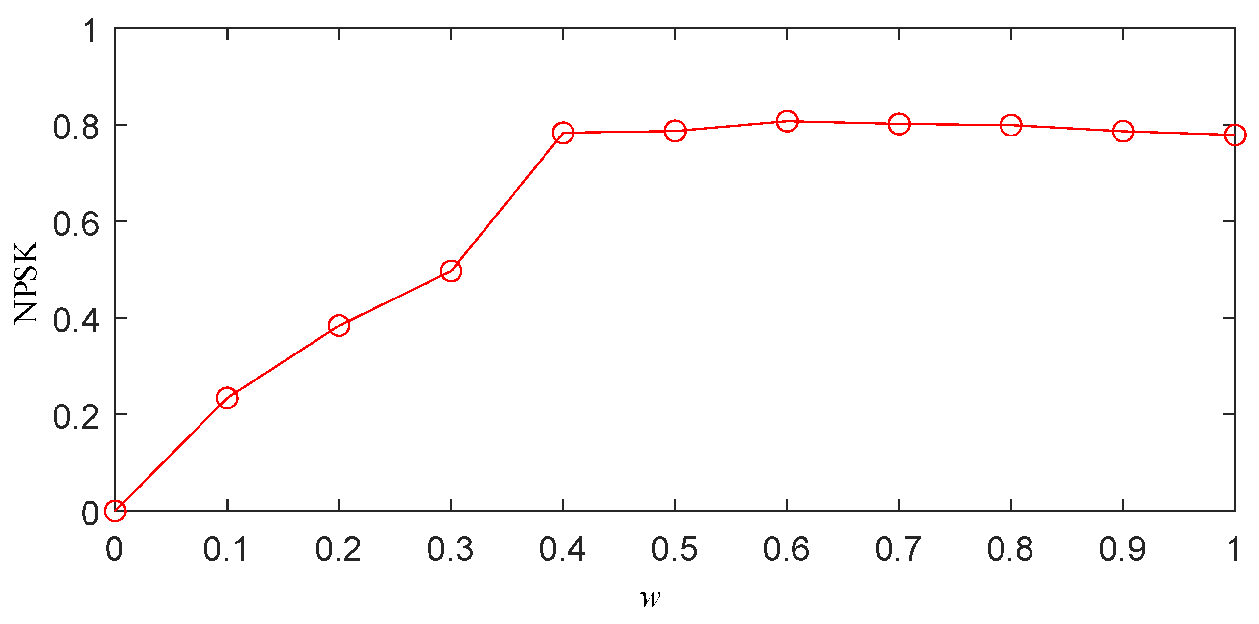
- Threshold selection based on normalized PSK (NPSK): The optimal segmentation threshold w ∈ [0, 1] is determined through the following:
- (1)
- Grid Search: The interval [0, 1] is discretized with Δw = 0.1 resolution, computing segmented frequency bands for each w value.
- (2)
- NPSK Calculation: For each segmentation result, the average PSK value across all frequency bands is calculated and normalized:Discrete determination criterion for optimal threshold w: For ordered discrete points forming a polyline, the transition point satisfieswhere and .The optimal threshold corresponds to the maximum slope variation point:where .
- (3)
- Power spectrum segmentation: The optimal threshold w is applied to the segmentation algorithm to obtain the best power spectrum segmentation results.
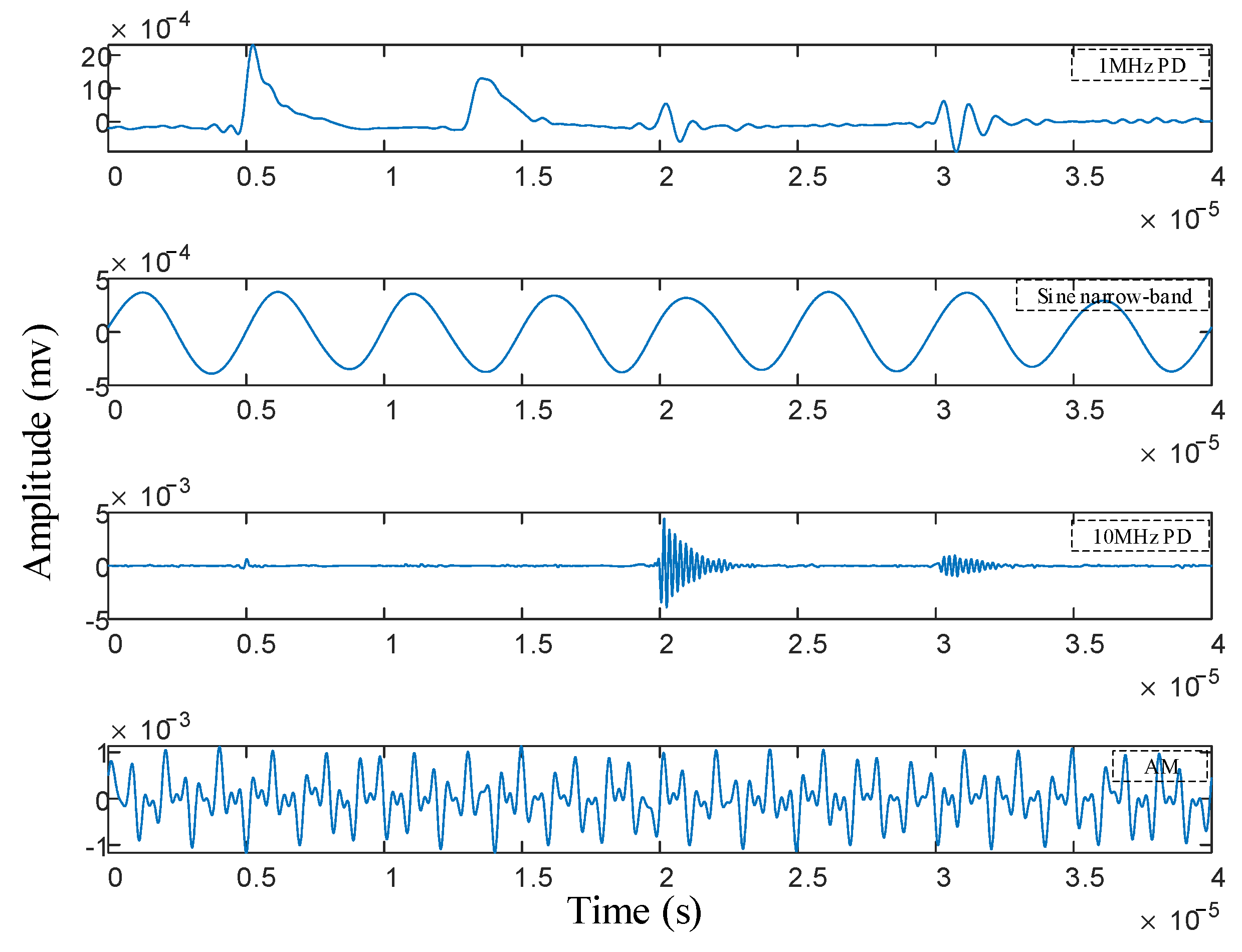
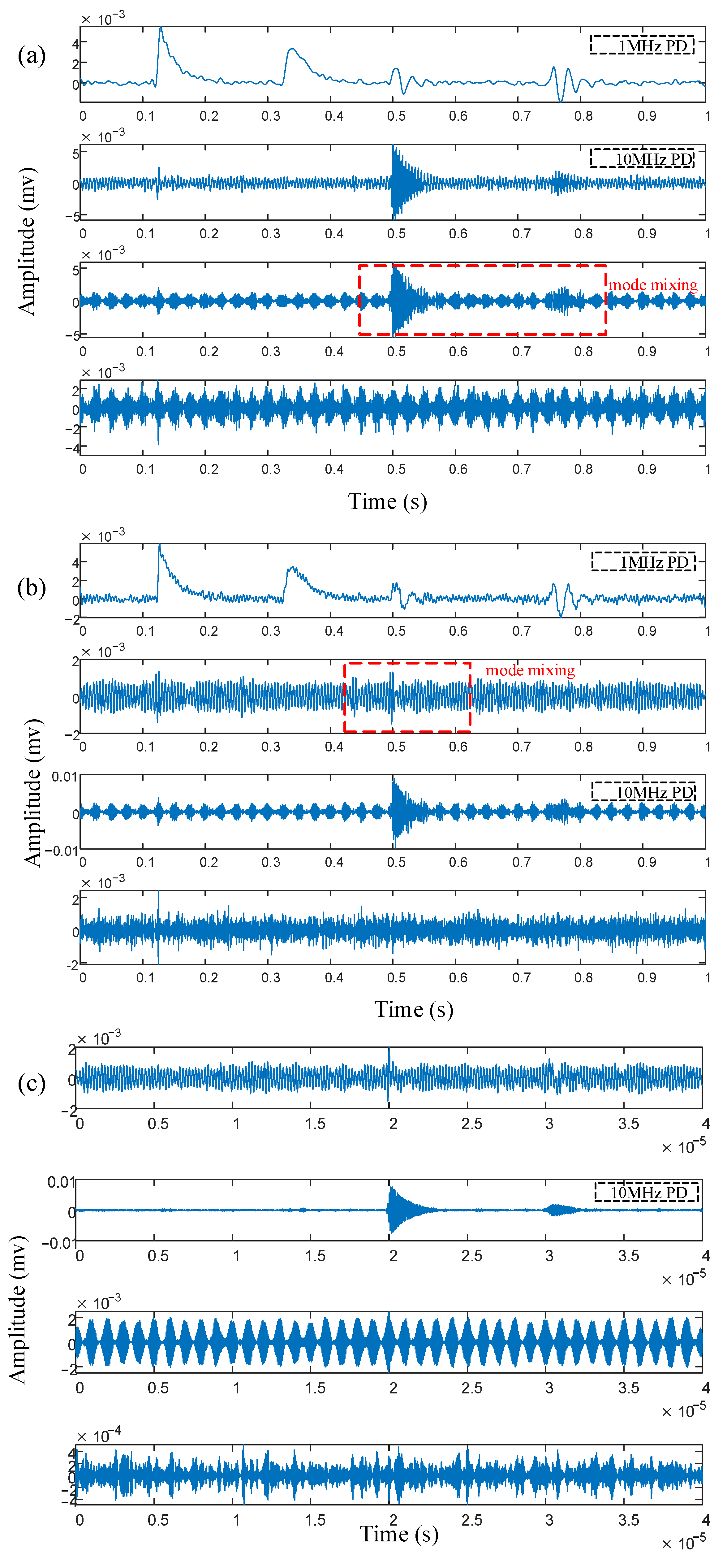
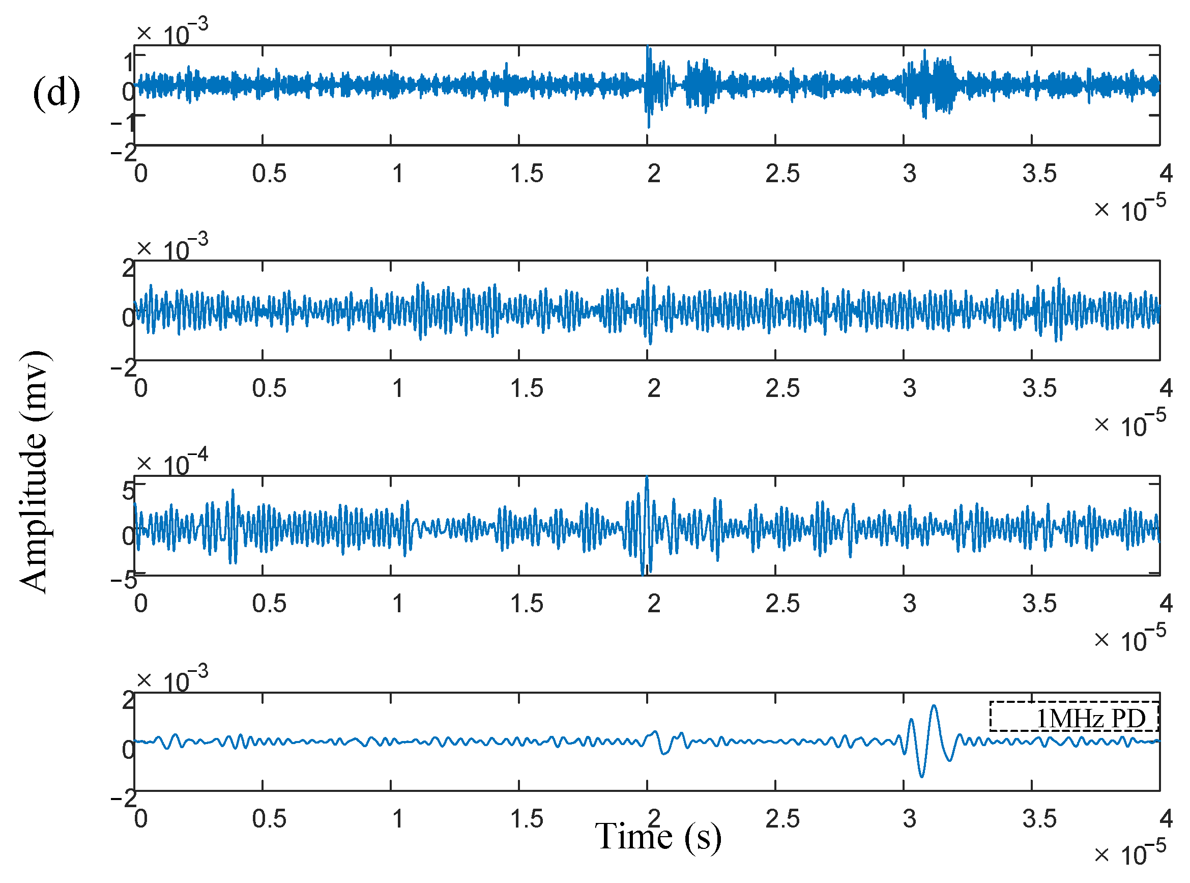
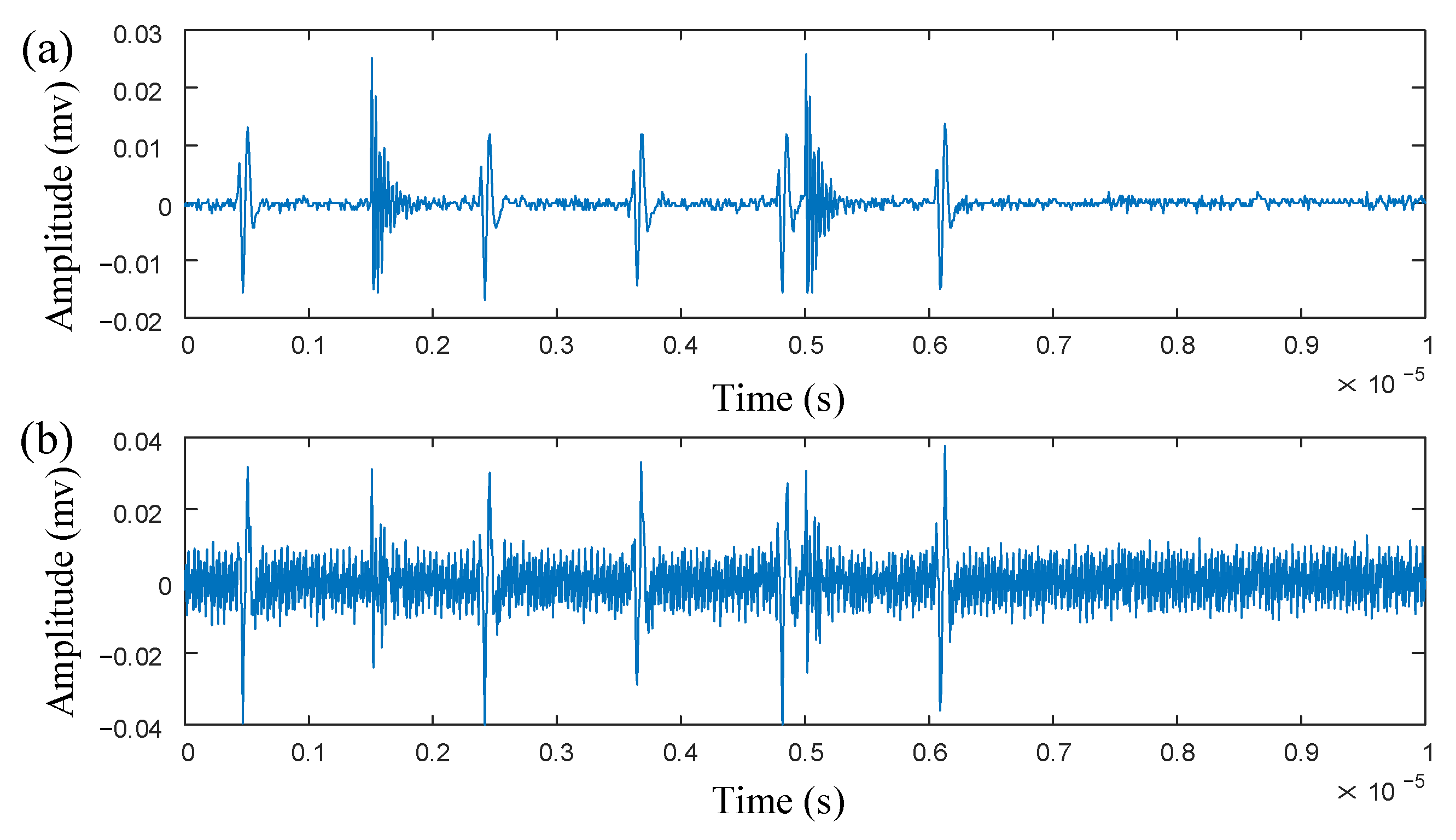
3. Simulation Analysis
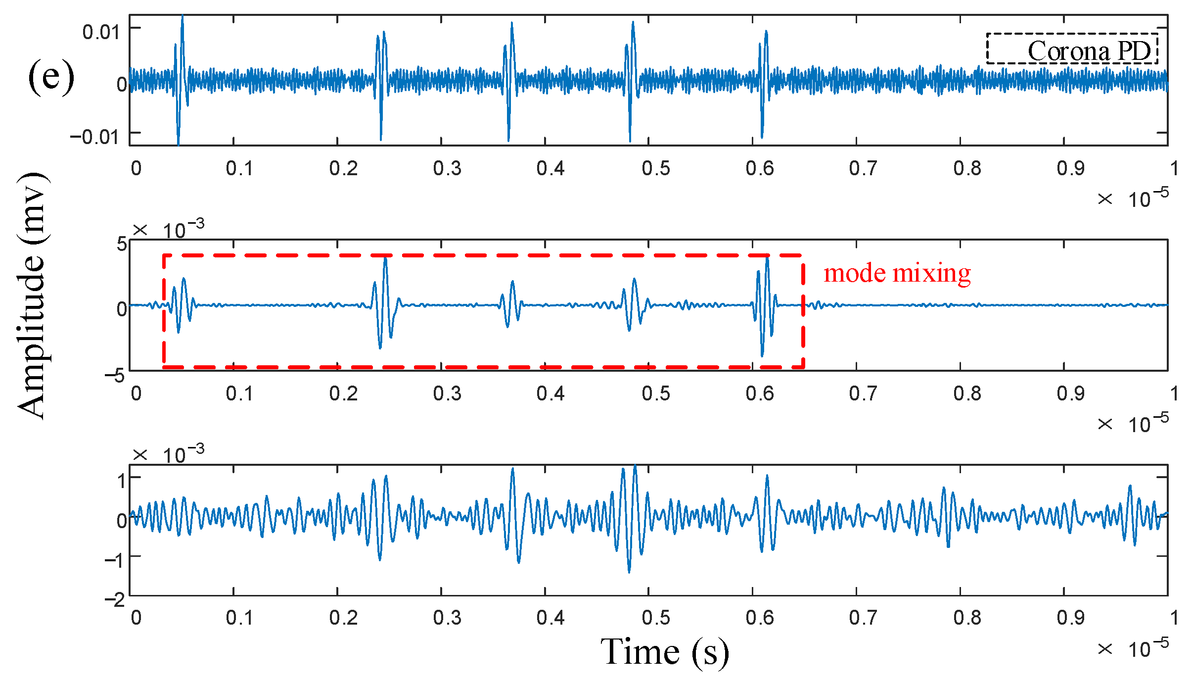
4. Analysis of Measured Signal
5. Conclusions
Author Contributions
Funding
Institutional Review Board Statement
Informed Consent Statement
Data Availability Statement
Conflicts of Interest
Abbreviations
| IPSK | Improved power spectral segmentation based on spectral kurtosis |
| PD | Partial discharge |
| EWT | Empirical wavelet transform |
| VMD | Variational mode decomposition |
| AEFD | Adaptive empirical Fourier decomposition |
| CEEMDAN | Complete ensemble empirical mode decomposition with adaptive noise |
| PSK | Power spectral kurtosis |
| NPSK | Normalized power spectral kurtosis |
References
- Zhao, Y.; Zhang, W.J.; Belhora, F. Intelligent Monitoring Technology of Partial Discharge Based on an Integrated Sensing-Memory-Computation System. Langmuir 2025, 41, 4976–4988. [Google Scholar] [CrossRef] [PubMed]
- Ayubi, B.I.; Zhang, L.; Wang, G.; Wang, Y.; Zhou, S. Molecular dynamics and finite element analysis of partial discharge mechanisms in polyimide under high-frequency electric stress. Polym. Degrad. Stab. 2025, 234, 111252. [Google Scholar] [CrossRef]
- Li, J.; Zhang, Q. A Method for Reducing White Noise in Partial Discharge Signals of Underground Power Cables. Electronics 2025, 14, 780. [Google Scholar] [CrossRef]
- Huang, N.E.; Long, S.R.; Wu, M.C.; Shih, H.H.; Zheng, Q.; Yen, N.C.; Tung, C.C.; Liu, H.H. The empirical mode decomposition and the hilbert spectrum for nonlinear and non-stationary time series analysis. Proc. R. Soc. Lond. Ser. A Math. Phys. Eng. Sci. 1998, 454, 903–995. [Google Scholar] [CrossRef]
- Jin, T.; Li, Q.; Mohamed, M.A. A novel adaptive EEMD method for switchgear partial discharge signal denoising. IEEE Access 2019, 7, 58139–58147. [Google Scholar] [CrossRef]
- Sun, K.; Li, W.; Zhang, J. Extraction and Application of Complex Noisy Partial Discharge Signals Containing Narrowband Noise and White Noise. J. Univ. Electron. Sci. Technol. China 2021, 50, 14–23. [Google Scholar]
- Dragomiretskiy, K.; Zosso, D. Variational Mode Decomposition. IEEE Trans. Signal Process. 2014, 62, 531–544. [Google Scholar] [CrossRef]
- Xia, Q.; Xiao, S.; Zhou, G.; Shang, Z.T.; Chen, B. Application of Improved VMD and Lifting Wavelet in Partial Discharge Denoising. Electr. Autom. 2022, 44, 46–48+52. [Google Scholar]
- Xiao, H.; Wei, J.; Liu, H.; Li, Q.; Shi, Y.; Zhang, T. Identification method for power system low frequency oscillations based on improved VMD and Teager-Kaiser energy operator. IET Gener. Transm. Distrib. 2017, 11, 4096–4103. [Google Scholar] [CrossRef]
- Nikolaou, N.G.; Antoniadis, I.A. Rolling element bearing fault diagnosis using wavelet packets. Ndt E Int. 2002, 35, 197–205. [Google Scholar] [CrossRef]
- Ma, X.H.; Zhang, D.K. Research on Suppression of Partial Discharge Noise of High Voltage Cable Based on Improved Empirical Wavelet Transform. Trans. China Electrotech. Soc. 2021, 36, 353–361. [Google Scholar]
- Zheng, J.; Pan, H.; Cheng, J. Adaptive Empirical Fourier Decomposition Based Mechanical Fault Diagnosis Method. J. Mech. Eng. 2020, 56, 125–136. [Google Scholar]
- Zheng, J.; Ying, W.; Pan, H. Fault Diagnosis Method of Rotating Machinery Based on Improved Holo-Hilbert Spectral Analysis. J. Mech. Eng. 2023, 59, 162–174. [Google Scholar]
- Yin, H.; Liu, W.; Xue, Q.; Song, C.; Ren, J.; Li, Z.; Wang, D.; Wang, K.; Han, D.; Yan, R. The value of restriction spectrum imaging in predicting lymph node metastases in rectal cancer: A comparative study with diffusion-weighted imaging and diffusion kurtosis imaging. Insights Imaging 2024, 15, 302. [Google Scholar] [CrossRef] [PubMed]
- Hussein, R.; Shaban, K.B.; El-Hag, A.H. Denoising different types of acoustic partial discharge signals using power spectral subtraction. High Volt. 2018, 3, 44–50. [Google Scholar] [CrossRef]
- Luo, R.P.; Luo, Y.T.; Lai, S.Y. Pattern Recognition of Partial Discharge Based on EEMD Singular Value Entropy. Appl. Electron. Tech. 2024, 50, 53–58. [Google Scholar]
- Xu, Y.C.; Xia, H.T.; Li, Z.H. Multi-Level Threshold Transformer Partial Discharge Noise Suppression Method Based on Synchronous Compression Domain. High Volt. Appar. 2021, 57, 123–131. [Google Scholar]


| PD | /mV | /μm | /μm | /MHz |
|---|---|---|---|---|
| 10 | 2 | 3 | 10 | |
| 3 | 2 | 3 | 1 |
| Methods | SNR/dB | RMSE | NCC |
|---|---|---|---|
| IPSK | 8.941 | 0.961 | |
| EWT | 4.665 | 0.856 | |
| AEFD | 4.973 | 0.879 | |
| VMD | 3.692 | 0.794 | |
| CEEMDAN | 4.455 | 0.711 |
Disclaimer/Publisher’s Note: The statements, opinions and data contained in all publications are solely those of the individual author(s) and contributor(s) and not of MDPI and/or the editor(s). MDPI and/or the editor(s) disclaim responsibility for any injury to people or property resulting from any ideas, methods, instructions or products referred to in the content. |
© 2025 by the authors. Licensee MDPI, Basel, Switzerland. This article is an open access article distributed under the terms and conditions of the Creative Commons Attribution (CC BY) license (https://creativecommons.org/licenses/by/4.0/).
Share and Cite
Chen, B.; Li, K.; Guo, Y. Effective Denoising of Multi-Source Partial Discharge Signals via an Improved Power Spectrum Segmentation Method Based on Normalized Spectral Kurtosis. Sensors 2025, 25, 3798. https://doi.org/10.3390/s25123798
Chen B, Li K, Guo Y. Effective Denoising of Multi-Source Partial Discharge Signals via an Improved Power Spectrum Segmentation Method Based on Normalized Spectral Kurtosis. Sensors. 2025; 25(12):3798. https://doi.org/10.3390/s25123798
Chicago/Turabian StyleChen, Baojia, Kaiwen Li, and Yipeng Guo. 2025. "Effective Denoising of Multi-Source Partial Discharge Signals via an Improved Power Spectrum Segmentation Method Based on Normalized Spectral Kurtosis" Sensors 25, no. 12: 3798. https://doi.org/10.3390/s25123798
APA StyleChen, B., Li, K., & Guo, Y. (2025). Effective Denoising of Multi-Source Partial Discharge Signals via an Improved Power Spectrum Segmentation Method Based on Normalized Spectral Kurtosis. Sensors, 25(12), 3798. https://doi.org/10.3390/s25123798