Author Contributions
Conceptualization, Y.L.; formal analysis, B.H., Z.X. and Y.L.; funding acquisition, Y.L.; investigation, B.H., Z.X. and Y.L.; methodology, B.H., Z.X. and Y.L.; resources, Y.L.; software, B.H., Z.X. and J.H.; supervision, Y.L.; validation, B.H., Z.X. and Y.L.; writing—original draft preparation, B.H.; writing—review and editing, B.H., Z.X., F.Y., Y.Z., Y.L., J.H. and J.B. All authors have read and agreed to the published version of the manuscript.
Figure 1.
Architecture of mmWave UAV A2G communications network.
Figure 1.
Architecture of mmWave UAV A2G communications network.
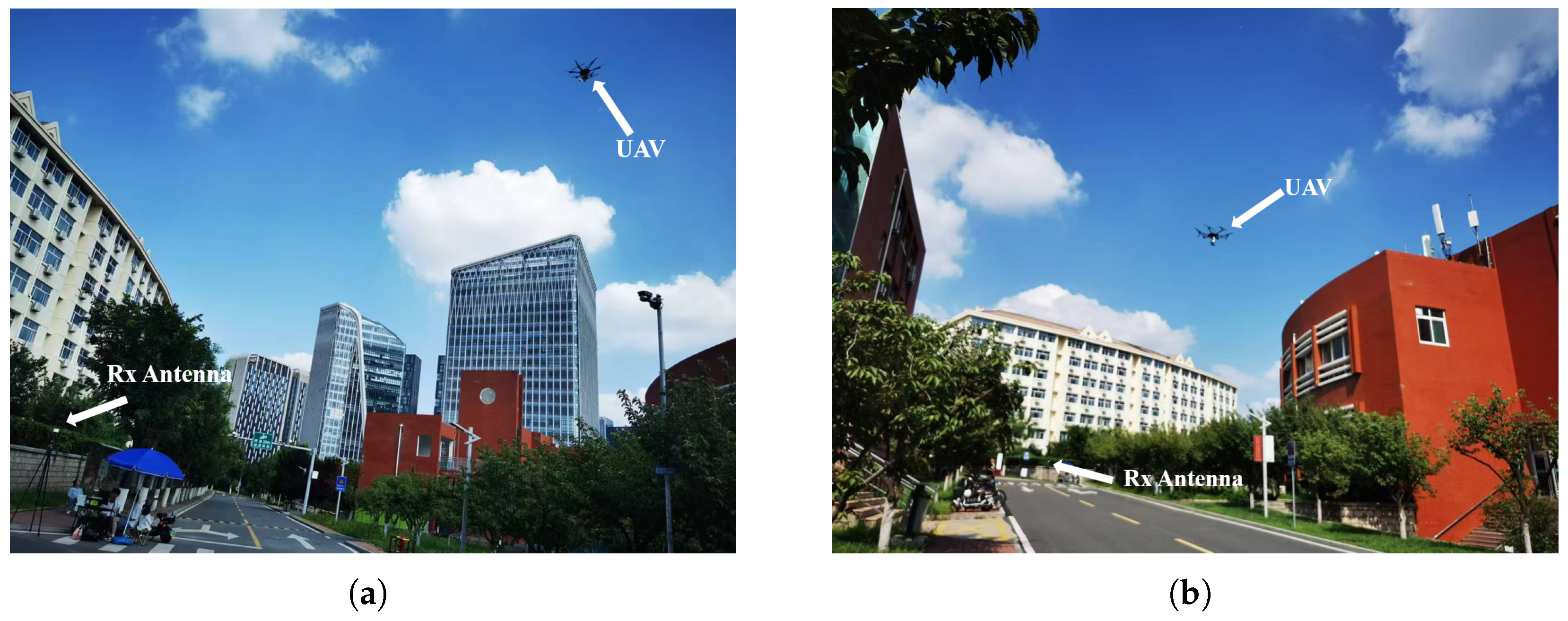
Figure 2.
Illustration of UAV air-to-ground channel measurements. (a) Measurement scenario 1. (b) Measurement scenario 2.
Figure 2.
Illustration of UAV air-to-ground channel measurements. (a) Measurement scenario 1. (b) Measurement scenario 2.
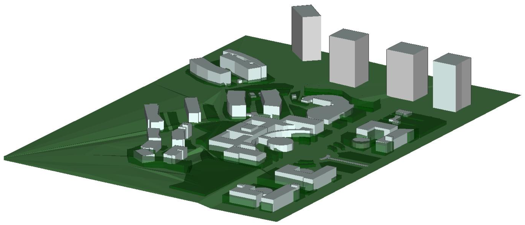
Figure 3.
Three-dimensional simulation environment for the campus scenario.
Figure 3.
Three-dimensional simulation environment for the campus scenario.
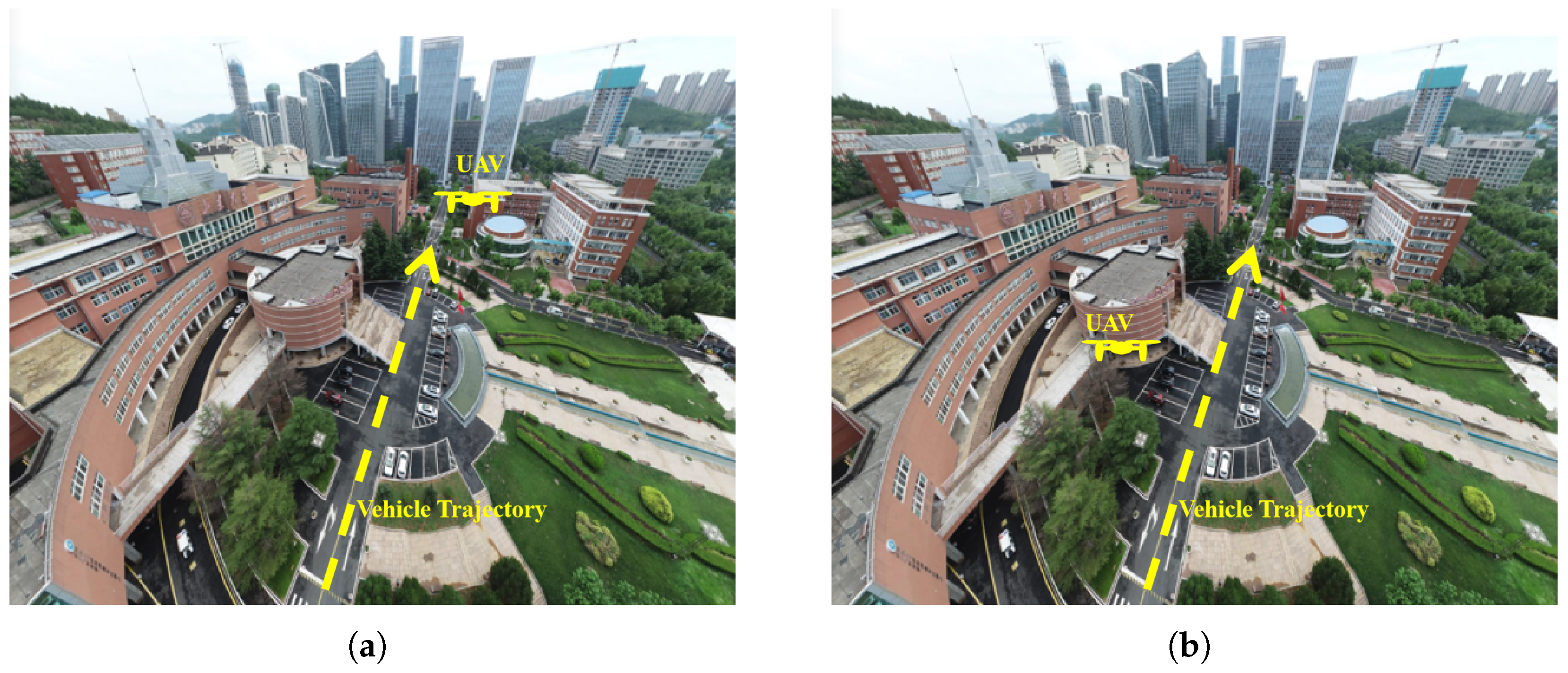
Figure 4.
The image of actual campus scenario acquired by UAV. (a) Relative position of UAV and vehicle at flight position 1. (b) Relative position of UAV and vehicle at flight position 2.
Figure 4.
The image of actual campus scenario acquired by UAV. (a) Relative position of UAV and vehicle at flight position 1. (b) Relative position of UAV and vehicle at flight position 2.
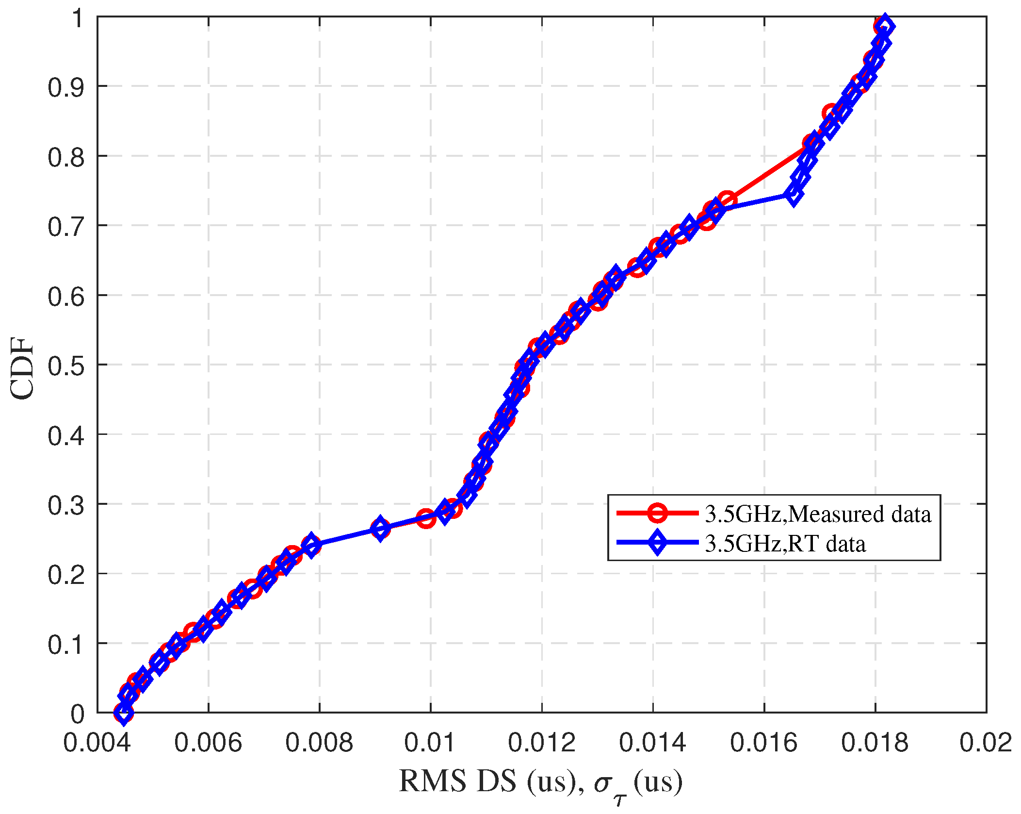
Figure 5.
Comparison of measured data and RT data for RMS DS at 3.5 GHz.
Figure 5.
Comparison of measured data and RT data for RMS DS at 3.5 GHz.
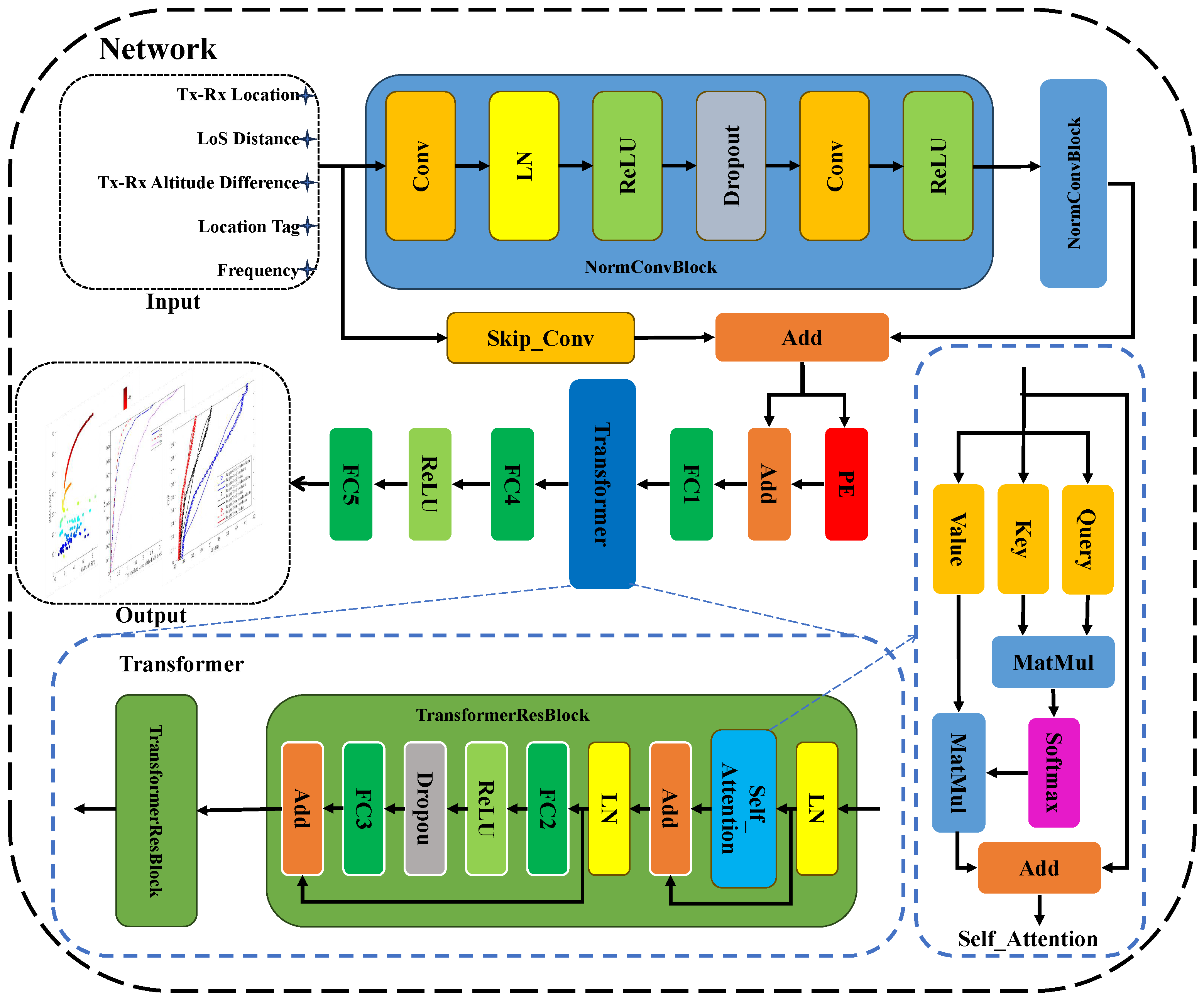
Figure 6.
The network structure of the channel prediction.
Figure 6.
The network structure of the channel prediction.
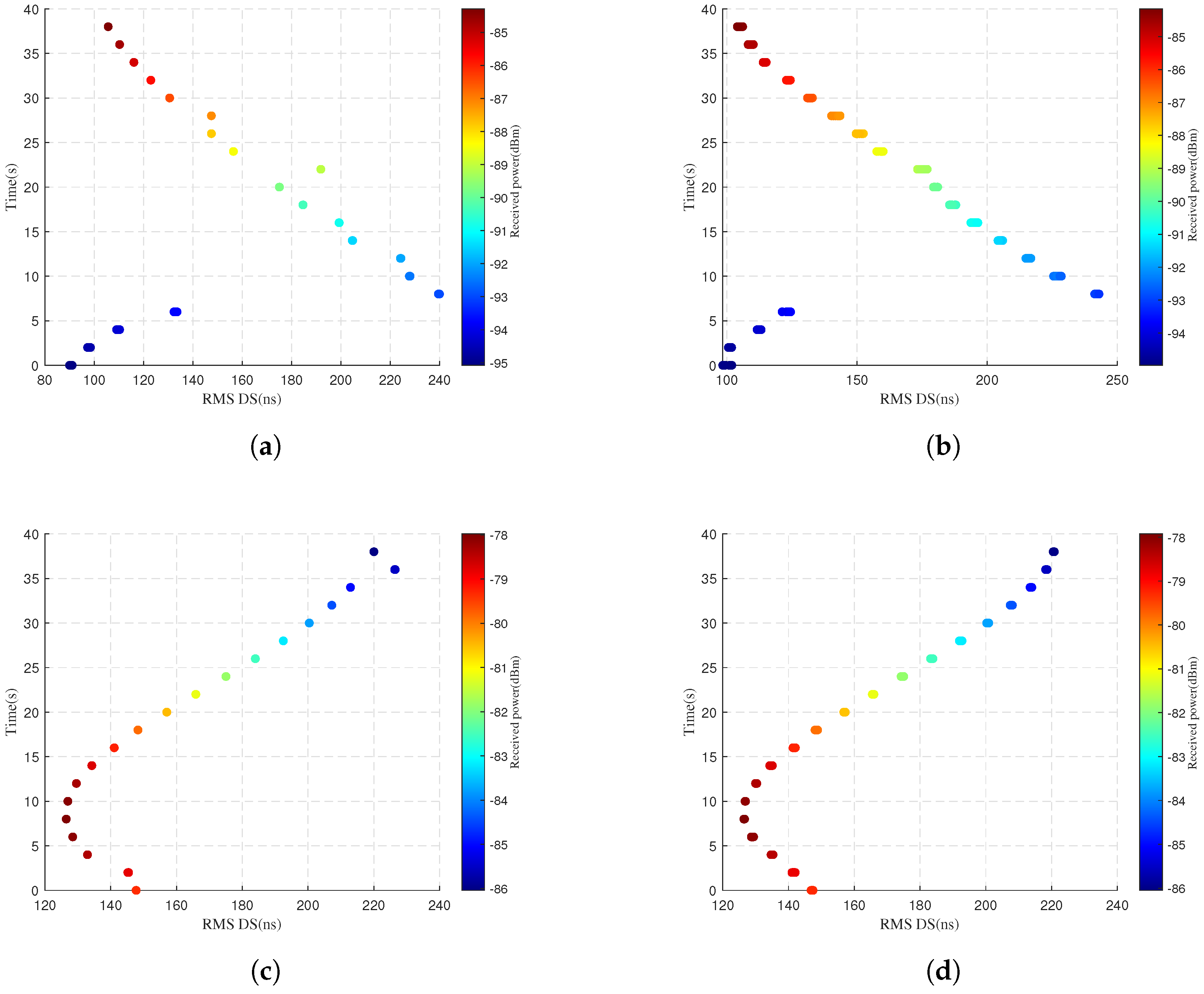
Figure 7.
Comparison of RMS DS and received power at different flight positions. Simulation values are displayed in the left column, while predicted values are presented in the right column. (a) Actual flight position 1. (b) Predicted flight position 1. (c) Actual flight position 2. (d) Predicted flight position 2.
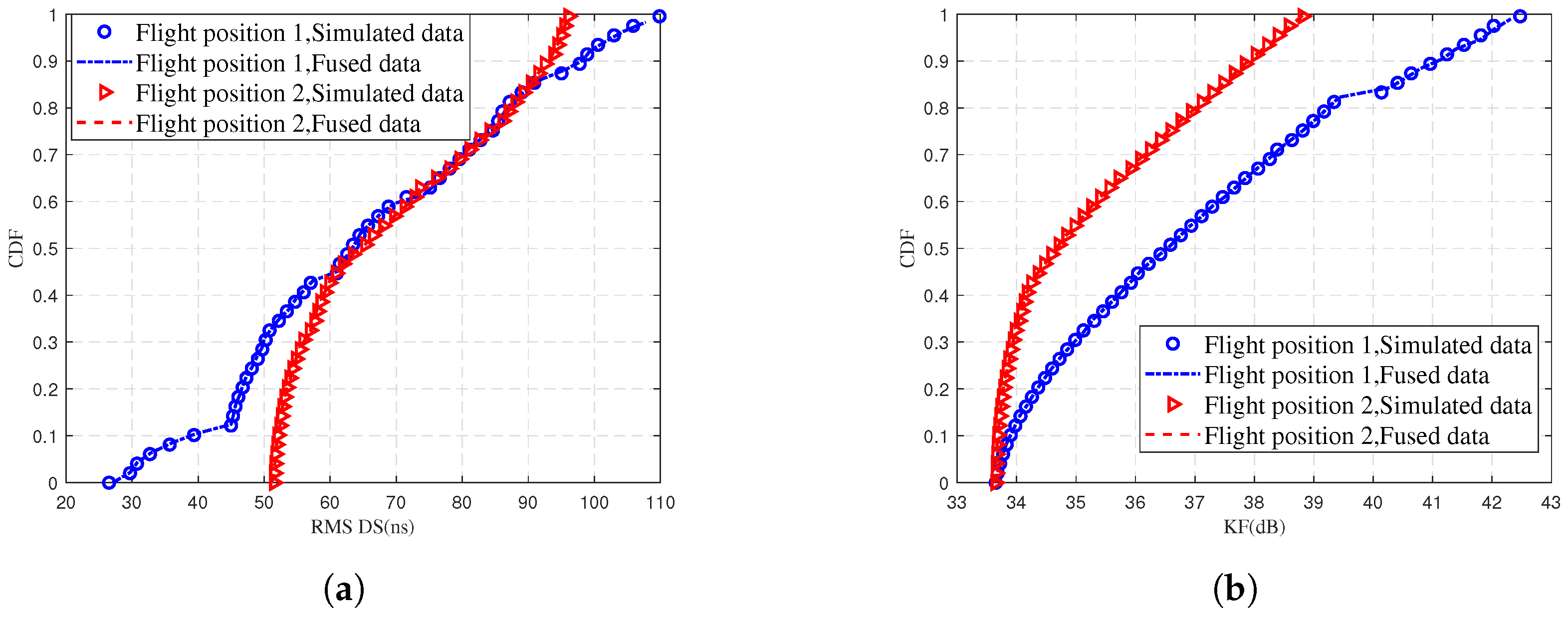
Figure 8.
Comparison of simulated data and fused data for (a) RMS DS and (b) KF at different UAV flight positions.
Figure 8.
Comparison of simulated data and fused data for (a) RMS DS and (b) KF at different UAV flight positions.
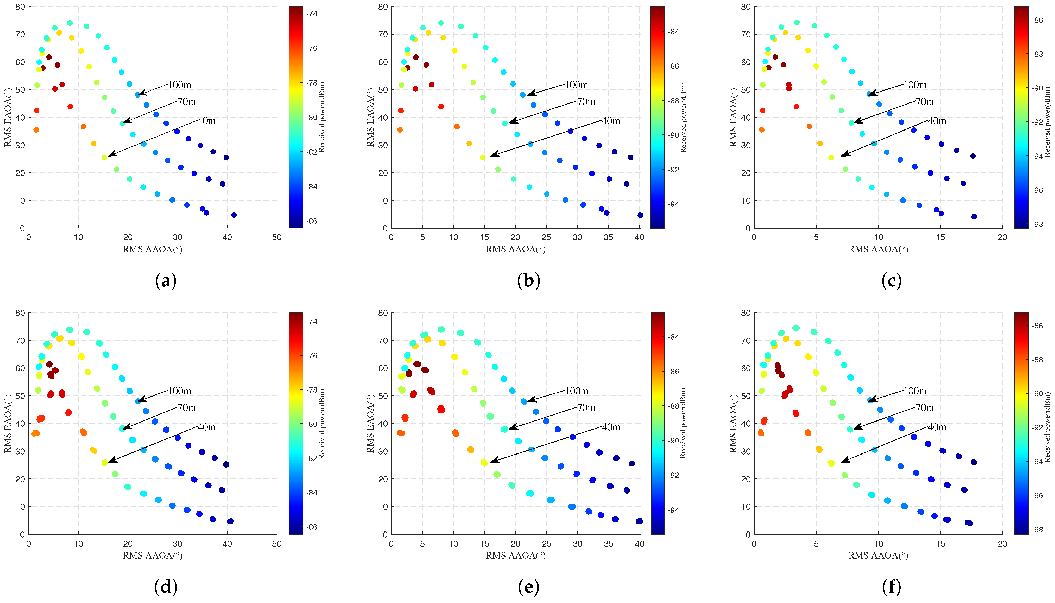
Figure 9.
Comparison of RMS AOA and received power at different flight altitudes. Simulated values are displayed in the first row, while predicted values are presented in the second row. (a) Actual 10 GHz. (b) Actual 28 GHz. (c) Actual 38 GHz. (d) Predicted 10 GHz. (e) Predicted 28 GHz. (f) Predicted 38 GHz.
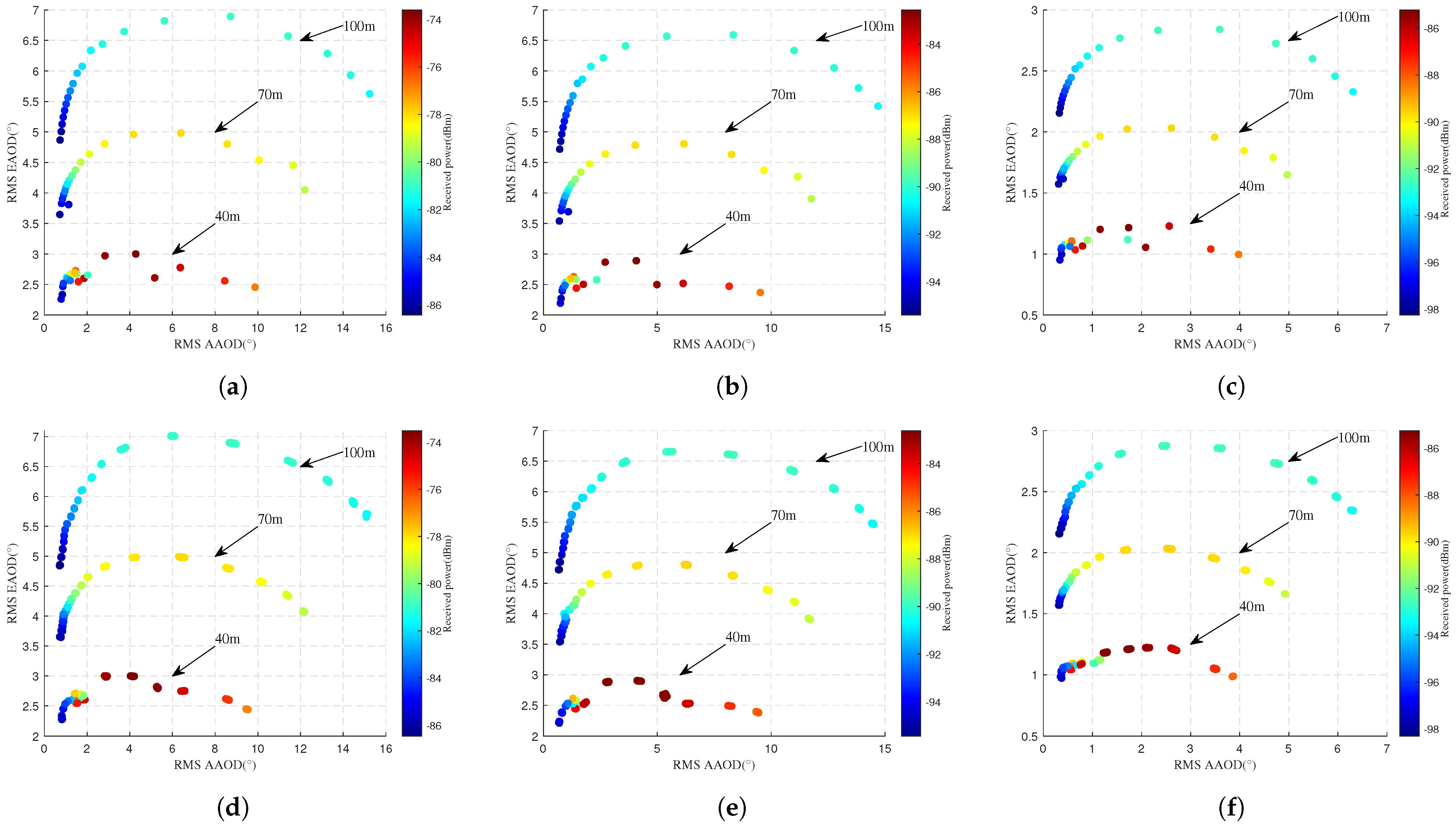
Figure 10.
Comparison of RMS AOD and received power at different flight altitudes. Simulated values are displayed in the first row, while predicted values are presented in the second row. (a) Actual 10 GHz. (b) Actual 28 GHz. (c) Actual 38 GHz. (d) Predicted 10 GHz. (e) Predicted 28 GHz. (f) Predicted 38 GHz.
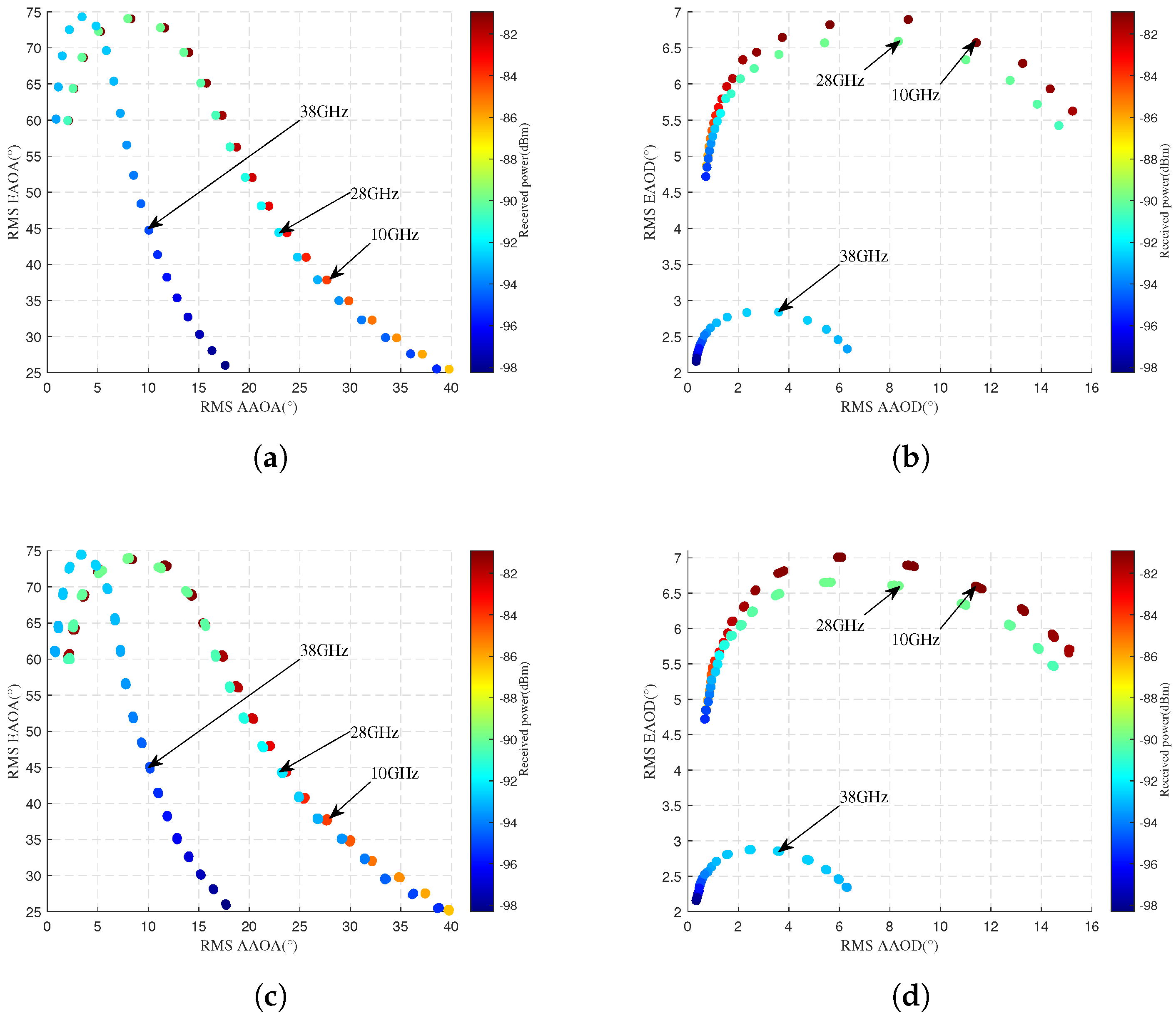
Figure 11.
Comparison of angle and received power at different flight altitudes. Simulated values are displayed in the first row, while the predicted values are presented in the second row. (a) Actual RMS AOA. (b) Actual RMS AOD. (c) Predicted RMS AOA. (d) Predicted RMS AOD.
Figure 11.
Comparison of angle and received power at different flight altitudes. Simulated values are displayed in the first row, while the predicted values are presented in the second row. (a) Actual RMS AOA. (b) Actual RMS AOD. (c) Predicted RMS AOA. (d) Predicted RMS AOD.
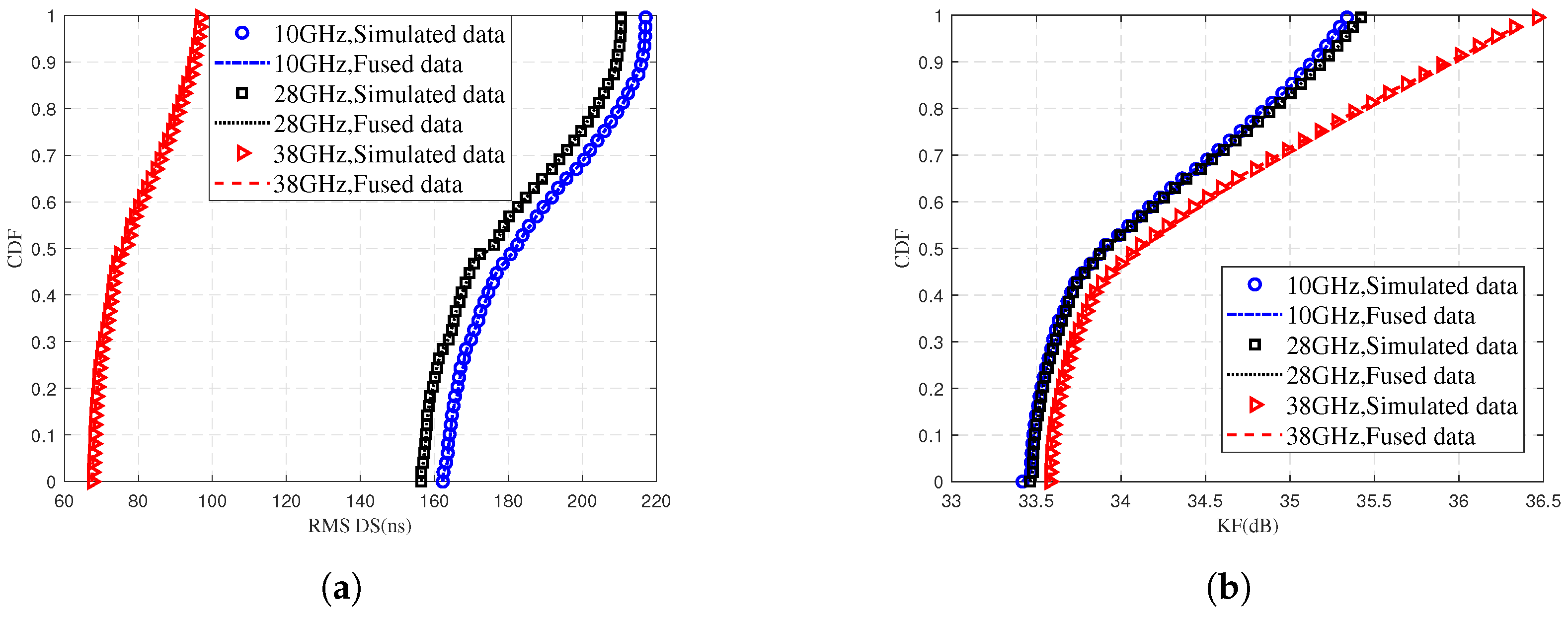
Figure 12.
Comparison of simulated data and fused data for (a) RMS DS and (b) KF at different communication frequencies.
Figure 12.
Comparison of simulated data and fused data for (a) RMS DS and (b) KF at different communication frequencies.
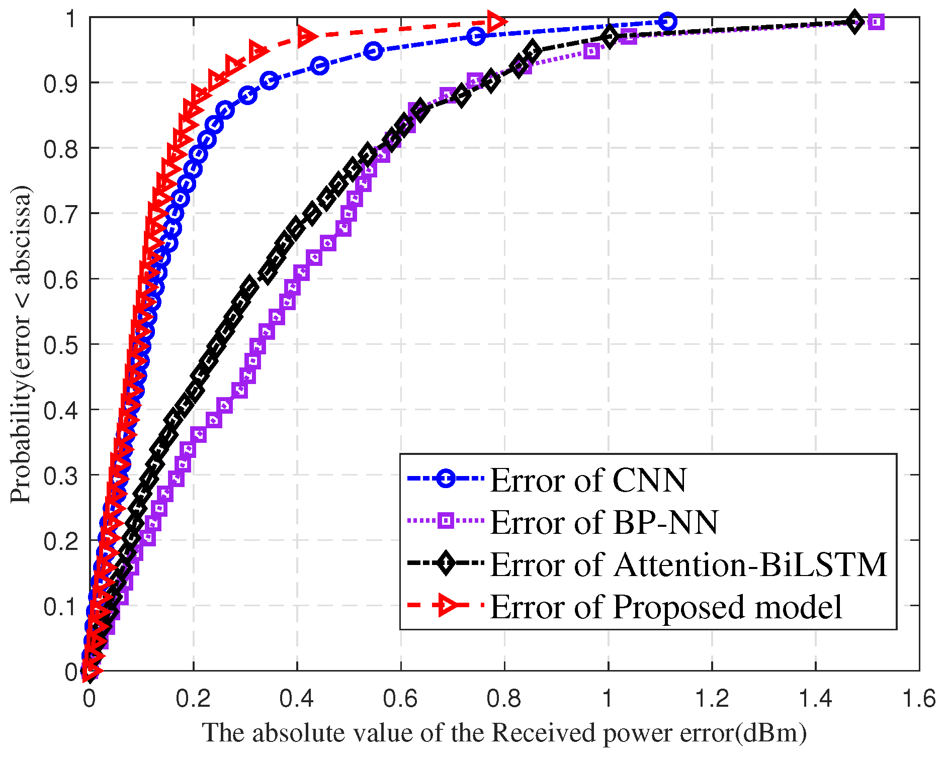
Figure 13.
Comparison of errors in received power prediction for different models.
Figure 13.
Comparison of errors in received power prediction for different models.
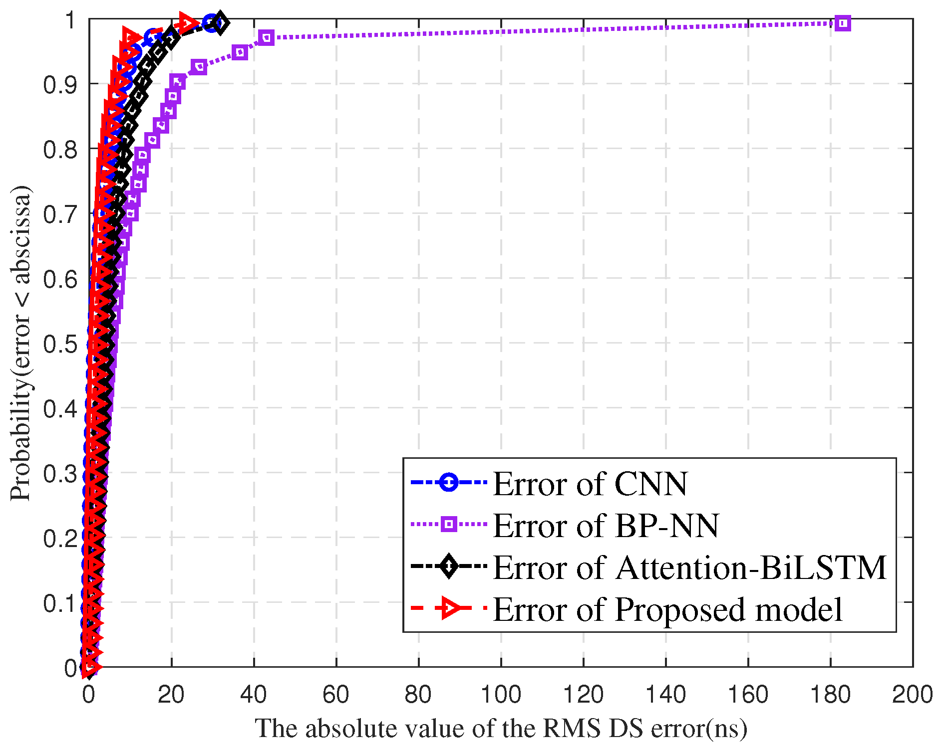
Figure 14.
Comparison of errors in RMS DS prediction for different models.
Figure 14.
Comparison of errors in RMS DS prediction for different models.
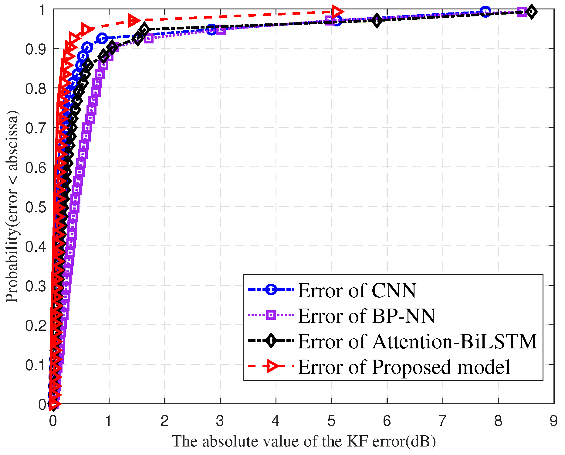
Figure 15.
Comparison of errors in KF prediction for different models.
Figure 15.
Comparison of errors in KF prediction for different models.
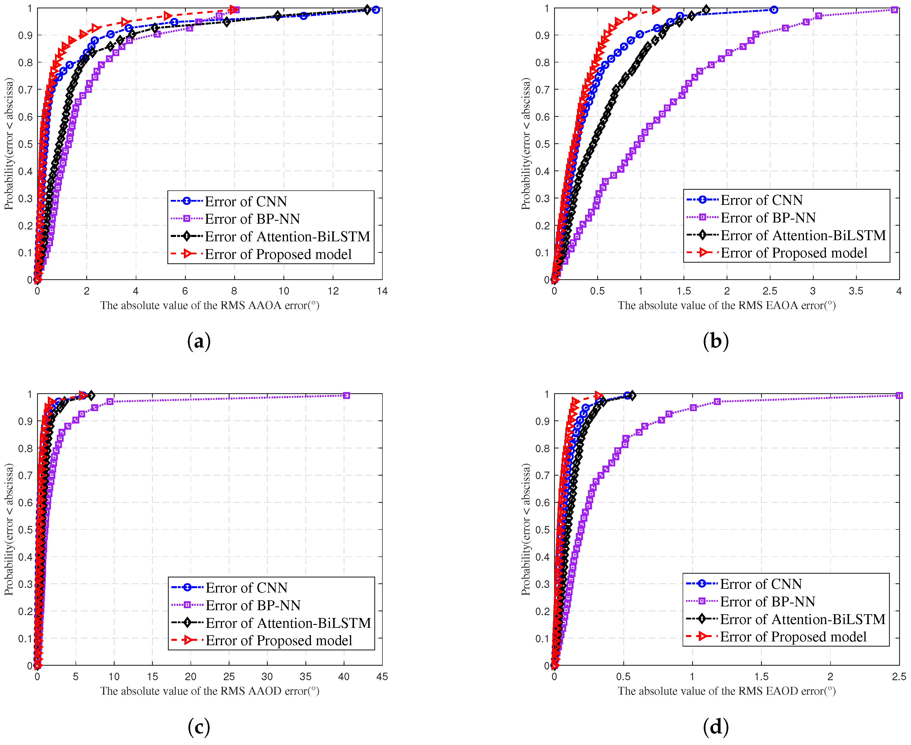
Figure 16.
Comparison of errors in (a) RMS AAOA prediction, (b) RMS EAOA prediction, (c) RMS AAOD prediction, and (d) RMS EAOD for different models.
Figure 16.
Comparison of errors in (a) RMS AAOA prediction, (b) RMS EAOA prediction, (c) RMS AAOD prediction, and (d) RMS EAOD for different models.
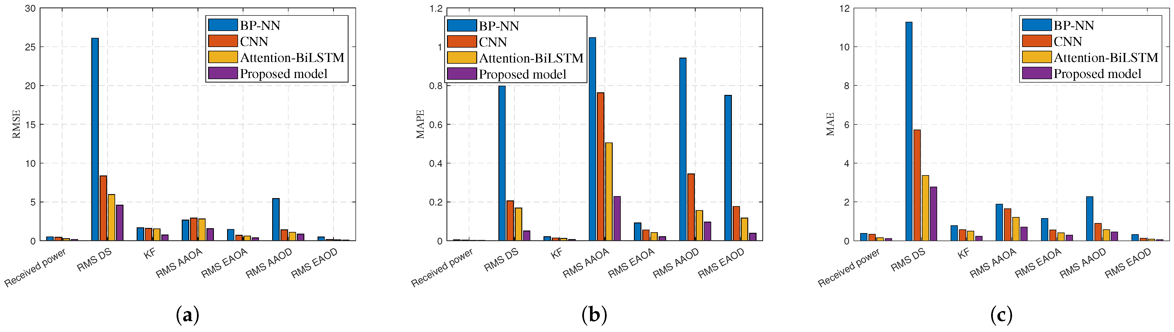
Figure 17.
Comparison of (a) RMSE, (b) MAPE, and (c) MAE for BP-NN, CNN, Attention-BiLSTM, and the proposed model using bar charts.
Figure 17.
Comparison of (a) RMSE, (b) MAPE, and (c) MAE for BP-NN, CNN, Attention-BiLSTM, and the proposed model using bar charts.
Table 1.
The details of material parameters.
Table 1.
The details of material parameters.
| Material | Permittivity | Conductivity (S/m) | Thickness (m) |
|---|
| Wet earth | 25 | 0.02 | 0 |
| Sea water | 81 | 20 | 0 |
| Concrete | 7 | 0.015 | 0.3 |
Table 2.
The details of simulation parameters.
Table 2.
The details of simulation parameters.
| Scenario | Flight Position 1 | Flight Position 2 |
|---|
| Frequency | 10 GHz/28 GHz/38 GHz | 10 GHz/28 GHz/38 GHz |
| Bandwidth | 500 MHz | 500 MHz |
| Transmit Power | 10 dBm | 10 dBm |
| Flight Altitude | 40 m/70 m/100 m | 40 m/70 m/100 m |
| Flight Trajectory | Hover | Hover |
| Vehicle Travel Distance | 199 m | 199 m |
| Travel Speed | 5 m/s | 5 m/s |
| Antenna Pattern | 2 × 2 antenna array | 2 × 2 antenna array |
| Reflection/Diffraction/Transmission | 6/1/0 | 6/1/0 |
Table 3.
The details of the proposed model.
Table 3.
The details of the proposed model.
| Parameter | Value |
|---|
| Conv Kernel Size | 4 × 4 |
| Dimension of Conv | 64 |
| Dropout | 0.01 |
| Dimension of FC1 | input: 64, output: 11 |
| Dimension of FC2 | input: 11, output: 33 |
| Dimension of FC3 | input: 33, output: 11 |
| Dimension of FC4 | input: 11, output: 64 |
| Dimension of FC5 | input: 64, output: 7 |
| Dimension of Self-Attention Head | 6 |
| Dimension of Q, K, and V | 32 |
Table 4.
Comparison of quantitative results of RMS DS at UAV flight position 1 for different communication frequencies and different flight altitudes.
Table 4.
Comparison of quantitative results of RMS DS at UAV flight position 1 for different communication frequencies and different flight altitudes.
| Frequency | Flight Altitude | RMSE (ns) | MAPE | MAE (ns) |
|---|
| 10 GHz | 40 m | 7.231 | 0.032 | 4.986 |
| 70 m | 5.841 | 0.028 | 4.167 |
| 100 m | 8.449 | 0.084 | 5.745 |
| 28 GHz | 40 m | 8.871 | 0.035 | 4.938 |
| 70 m | 4.075 | 0.020 | 2.615 |
| 100 m | 10.190 | 0.102 | 6.711 |
| 38 GHz | 40 m | 5.806 | 0.058 | 2.615 |
| 70 m | 1.345 | 0.016 | 0.924 |
| 100 m | 6.638 | 0.193 | 4.127 |
Table 5.
Comparison of quantitative results of RMS DS at UAV flight position 2 for different communication frequencies and different flight altitudes.
Table 5.
Comparison of quantitative results of RMS DS at UAV flight position 2 for different communication frequencies and different flight altitudes.
| Frequency | Flight Altitude | RMSE (ns) | MAPE | MAE (ns) |
|---|
| 10 GHz | 40 m | 3.117 | 0.015 | 2.212 |
| 70 m | 2.098 | 0.006 | 1.046 |
| 100 m | 1.648 | 0.006 | 0.938 |
| 28 GHz | 40 m | 2.950 | 0.015 | 2.170 |
| 70 m | 1.855 | 0.006 | 0.989 |
| 100 m | 0.969 | 0.004 | 0.673 |
| 38 GHz | 40 m | 1.339 | 0.018 | 1.006 |
| 70 m | 0.470 | 0.004 | 0.302 |
| 100 m | 0.429 | 0.004 | 0.311 |
Table 6.
Comparison of quantitative results of KF at UAV flight position 1 for different communication frequencies and different flight altitudes.
Table 6.
Comparison of quantitative results of KF at UAV flight position 1 for different communication frequencies and different flight altitudes.
| Frequency | Flight Altitude | RMSE (dB) | MAPE | MAE (dB) |
|---|
| 10 GHz | 40 m | 1.458 | 0.025 | 0.996 |
| 70 m | 0.125 | 0.002 | 0.087 |
| 100 m | 0.088 | 0.002 | 0.066 |
| 28 GHz | 40 m | 2.529 | 0.033 | 1.371 |
| 70 m | 0.117 | 0.002 | 0.075 |
| 100 m | 0.082 | 0.002 | 0.055 |
| 38 GHz | 40 m | 2.113 | 0.032 | 1.351 |
| 70 m | 0.105 | 0.002 | 0.069 |
| 100 m | 0.076 | 0.002 | 0.060 |
Table 7.
Comparison of quantitative results of KF at UAV flight position 2 for different communication frequencies and different flight altitudes.
Table 7.
Comparison of quantitative results of KF at UAV flight position 2 for different communication frequencies and different flight altitudes.
| Frequency | Flight Altitude | RMSE (dB) | MAPE | MAE (dB) |
|---|
| 10 GHz | 40 m | 0.063 | 0.0012 | 0.044 |
| 70 m | 0.013 | 0.0003 | 0.011 |
| 100 m | 0.011 | 0.0002 | 0.008 |
| 28 GHz | 40 m | 0.064 | 0.0013 | 0.049 |
| 70 m | 0.021 | 0.0005 | 0.017 |
| 100 m | 0.010 | 0.0002 | 0.008 |
| 38 GHz | 40 m | 0.065 | 0.0014 | 0.051 |
| 70 m | 0.017 | 0.0004 | 0.014 |
| 100 m | 0.013 | 0.0003 | 0.010 |
Table 8.
Comparison of quantitative results of received power at UAV flight position 1 for different communication frequencies and different flight altitudes.
Table 8.
Comparison of quantitative results of received power at UAV flight position 1 for different communication frequencies and different flight altitudes.
| Frequency | Flight Altitude | RMSE (dBm) | MAPE | MAE (dBm) |
|---|
| 10 GHz | 40 m | 0.316 | 0.003 | 0.262 |
| 70 m | 0.092 | 0.001 | 0.071 |
| 100 m | 0.130 | 0.001 | 0.095 |
| 28 GHz | 40 m | 0.351 | 0.002 | 0.227 |
| 70 m | 0.099 | 0.001 | 0.076 |
| 100 m | 0.094 | 0.001 | 0.076 |
| 38 GHz | 40 m | 0.287 | 0.002 | 0.199 |
| 70 m | 0.068 | 0.001 | 0.054 |
| 100 m | 0.086 | 0.001 | 0.063 |
Table 9.
Comparison of quantitative results of received power at UAV flight position 2 for different communication frequencies and different flight altitudes.
Table 9.
Comparison of quantitative results of received power at UAV flight position 2 for different communication frequencies and different flight altitudes.
| Frequency | Flight Altitude | RMSE (dBm) | MAPE | MAE (dBm) |
|---|
| 10 GHz | 40 m | 0.087 | 0.0009 | 0.072 |
| 70 m | 0.027 | 0.0003 | 0.022 |
| 100 m | 0.024 | 0.0002 | 0.018 |
| 28 GHz | 40 m | 0.107 | 0.0009 | 0.082 |
| 70 m | 0.036 | 0.0003 | 0.027 |
| 100 m | 0.026 | 0.0002 | 0.020 |
| 38 GHz | 40 m | 0.095 | 0.0009 | 0.077 |
| 70 m | 0.032 | 0.0003 | 0.023 |
| 100 m | 0.023 | 0.0002 | 0.019 |
Table 10.
Comparison of quantitative results of RMS AAOA at UAV flight position 1 for different communication frequencies and different flight altitudes.
Table 10.
Comparison of quantitative results of RMS AAOA at UAV flight position 1 for different communication frequencies and different flight altitudes.
| Frequency | Flight Altitude | RMSE (°) | MAPE | MAE (°) |
|---|
| 10 GHz | 40 m | 5.942 | 0.931 | 4.227 |
| 70 m | 1.919 | 0.634 | 1.371 |
| 100 m | 2.126 | 0.493 | 1.237 |
| 28 GHz | 40 m | 5.808 | 1.197 | 4.257 |
| 70 m | 1.282 | 0.478 | 0.864 |
| 100 m | 2.496 | 0.535 | 1.397 |
| 38 GHz | 40 m | 5.028 | 1.133 | 3.526 |
| 70 m | 0.404 | 0.405 | 0.290 |
| 100 m | 1.342 | 0.547 | 0.720 |
Table 11.
Comparison of quantitative results of RMS AAOA at UAV flight position 2 for different communication frequencies and different flight altitudes.
Table 11.
Comparison of quantitative results of RMS AAOA at UAV flight position 2 for different communication frequencies and different flight altitudes.
| Frequency | Flight Altitude | RMSE (°) | MAPE | MAE (°) |
|---|
| 10 GHz | 40 m | 0.591 | 0.081 | 0.416 |
| 70 m | 0.133 | 0.016 | 0.102 |
| 100 m | 0.147 | 0.011 | 0.115 |
| 28 GHz | 40 m | 0.513 | 0.055 | 0.373 |
| 70 m | 0.198 | 0.023 | 0.141 |
| 100 m | 0.208 | 0.014 | 0.165 |
| 38 GHz | 40 m | 0.313 | 0.092 | 0.206 |
| 70 m | 0.059 | 0.018 | 0.049 |
| 100 m | 0.088 | 0.019 | 0.074 |
Table 12.
Comparison of quantitative results of RMS EAOA at UAV flight position 1 for different communication frequencies and different flight altitudes.
Table 12.
Comparison of quantitative results of RMS EAOA at UAV flight position 1 for different communication frequencies and different flight altitudes.
| Frequency | Flight Altitude | RMSE (°) | MAPE | MAE (°) |
|---|
| 10 GHz | 40 m | 0.900 | 0.104 | 0.685 |
| 70 m | 0.814 | 0.026 | 0.633 |
| 100 m | 0.538 | 0.013 | 0.427 |
| 28 GHz | 40 m | 0.760 | 0.231 | 0.469 |
| 70 m | 0.505 | 0.023 | 0.354 |
| 100 m | 0.376 | 0.010 | 0.306 |
| 38 GHz | 40 m | 0.625 | 0.188 | 0.511 |
| 70 m | 0.542 | 0.016 | 0.310 |
| 100 m | 0.512 | 0.013 | 0.398 |
Table 13.
Comparison of quantitative results of RMS EAOA at UAV flight position 2 for different communication frequencies and different flight altitudes.
Table 13.
Comparison of quantitative results of RMS EAOA at UAV flight position 2 for different communication frequencies and different flight altitudes.
| Frequency | Flight Altitude | RMSE (°) | MAPE | MAE (°) |
|---|
| 10 GHz | 40 m | 0.483 | 0.017 | 0.368 |
| 70 m | 0.222 | 0.004 | 0.174 |
| 100 m | 0.260 | 0.004 | 0.205 |
| 28 GHz | 40 m | 0.472 | 0.013 | 0.327 |
| 70 m | 0.249 | 0.006 | 0.201 |
| 100 m | 0.221 | 0.004 | 0.177 |
| 38 GHz | 40 m | 0.543 | 0.013 | 0.353 |
| 70 m | 0.182 | 0.003 | 0.138 |
| 100 m | 0.287 | 0.004 | 0.195 |
Table 14.
Comparison of quantitative results of RMS AAOD at UAV flight position 1 for different communication frequencies and different flight altitudes.
Table 14.
Comparison of quantitative results of RMS AAOD at UAV flight position 1 for different communication frequencies and different flight altitudes.
| Frequency | Flight Altitude | RMSE (°) | MAPE | MAE (°) |
|---|
| 10 GHz | 40 m | 2.044 | 0.035 | 1.156 |
| 70 m | 0.782 | 0.021 | 0.570 |
| 100 m | 0.818 | 0.085 | 0.605 |
| 28 GHz | 40 m | 1.699 | 0.028 | 0.844 |
| 70 m | 0.601 | 0.016 | 0.416 |
| 100 m | 0.921 | 0.101 | 0.642 |
| 38 GHz | 40 m | 0.828 | 0.043 | 0.533 |
| 70 m | 0.245 | 0.014 | 0.153 |
| 100 m | 0.530 | 0.155 | 0.387 |
Table 15.
Comparison of quantitative results of RMS AAOD at UAV flight position 2 for different communication frequencies and different flight altitudes.
Table 15.
Comparison of quantitative results of RMS AAOD at UAV flight position 2 for different communication frequencies and different flight altitudes.
| Frequency | Flight Altitude | RMSE (°) | MAPE | MAE (°) |
|---|
| 10 GHz | 40 m | 0.206 | 0.087 | 0.150 |
| 70 m | 0.109 | 0.035 | 0.068 |
| 100 m | 0.113 | 0.024 | 0.072 |
| 28 GHz | 40 m | 0.255 | 0.095 | 0.158 |
| 70 m | 0.109 | 0.051 | 0.084 |
| 100 m | 0.087 | 0.021 | 0.057 |
| 38 GHz | 40 m | 0.189 | 0.133 | 0.113 |
| 70 m | 0.034 | 0.028 | 0.024 |
| 100 m | 0.039 | 0.029 | 0.027 |
Table 16.
Comparison of quantitative results of RMS EAOD at UAV flight position 1 for different communication frequencies and different flight altitudes.
Table 16.
Comparison of quantitative results of RMS EAOD at UAV flight position 1 for different communication frequencies and different flight altitudes.
| Frequency | Flight Altitude | RMSE (°) | MAPE | MAE (°) |
|---|
| 10 GHz | 40 m | 0.083 | 0.039 | 0.067 |
| 70 m | 0.106 | 0.026 | 0.080 |
| 100 m | 0.197 | 0.220 | 0.156 |
| 28 GHz | 40 m | 0.142 | 0.082 | 0.088 |
| 70 m | 0.081 | 0.020 | 0.056 |
| 100 m | 0.228 | 0.133 | 0.141 |
| 38 GHz | 40 m | 0.102 | 0.097 | 0.073 |
| 70 m | 0.028 | 0.017 | 0.021 |
| 100 m | 0.140 | 0.073 | 0.095 |
Table 17.
Comparison of quantitative results of RMS EAOD at UAV flight position 2 for different communication frequencies and different flight altitudes.
Table 17.
Comparison of quantitative results of RMS EAOD at UAV flight position 2 for different communication frequencies and different flight altitudes.
| Frequency | Flight Altitude | RMSE (°) | MAPE | MAE (°) |
|---|
| 10 GHz | 40 m | 0.054 | 0.012 | 0.031 |
| 70 m | 0.030 | 0.004 | 0.017 |
| 100 m | 0.063 | 0.006 | 0.038 |
| 28 GHz | 40 m | 0.044 | 0.012 | 0.029 |
| 70 m | 0.023 | 0.003 | 0.013 |
| 100 m | 0.033 | 0.004 | 0.022 |
| 38 GHz | 40 m | 0.041 | 0.021 | 0.022 |
| 70 m | 0.008 | 0.003 | 0.005 |
| 100 m | 0.017 | 0.004 | 0.012 |
Table 18.
Comparison of prediction performance in characteristics prediction for different models using merged datasets.
Table 18.
Comparison of prediction performance in characteristics prediction for different models using merged datasets.
| Channel Characteristic | Network | RMSE | MAPE | MAE |
|---|
| Received power (dBm) | Proposed model | 0.172 | 0.001 | 0.118 |
| BP-NN | 0.497 | 0.004 | 0.381 |
| CNN | 0.250 | 0.002 | 0.158 |
| Attention-BiLSTM | 0.448 | 0.004 | 0.331 |
| RMS DS (ns) | Proposed model | 4.577 | 0.050 | 2.769 |
| BP-NN | 26.112 | 0.797 | 11.267 |
| CNN | 5.961 | 0.169 | 3.370 |
| Attention-BiLSTM | 8.347 | 0.205 | 5.713 |
| KF (dB) | Proposed model | 0.745 | 0.006 | 0.226 |
| BP-NN | 1.675 | 0.020 | 0.776 |
| CNN | 1.538 | 0.012 | 0.502 |
| Attention-BiLSTM | 1.599 | 0.014 | 0.574 |
| RMS AAOA (°) | Proposed model | 1.549 | 0.229 | 0.708 |
| BP-NN | 2.666 | 1.047 | 1.882 |
| CNN | 2.811 | 0.505 | 1.198 |
| Attention-BiLSTM | 2.917 | 0.763 | 1.645 |
| RMS EAOA (°) | Proposed model | 0.375 | 0.021 | 0.285 |
| BP-NN | 1.458 | 0.092 | 1.147 |
| CNN | 0.608 | 0.042 | 0.408 |
| Attention-BiLSTM | 0.713 | 0.056 | 0.560 |
| RMS AAOD (°) | Proposed model | 0.864 | 0.096 | 0.450 |
| BP-NN | 5.432 | 0.941 | 2.265 |
| CNN | 1.094 | 0.156 | 0.574 |
| Attention-BiLSTM | 1.415 | 0.344 | 0.901 |
| RMS EAOD (°) | Proposed model | 0.074 | 0.039 | 0.053 |
| BP-NN | 0.496 | 0.749 | 0.317 |
| CNN | 0.123 | 0.116 | 0.082 |
| Attention-BiLSTM | 0.160 | 0.177 | 0.121 |


 ,
, 


