
Trends and Techniques in 3D Reconstruction and Rendering: A Survey with Emphasis on Gaussian Splatting


Abstract
1. Introduction
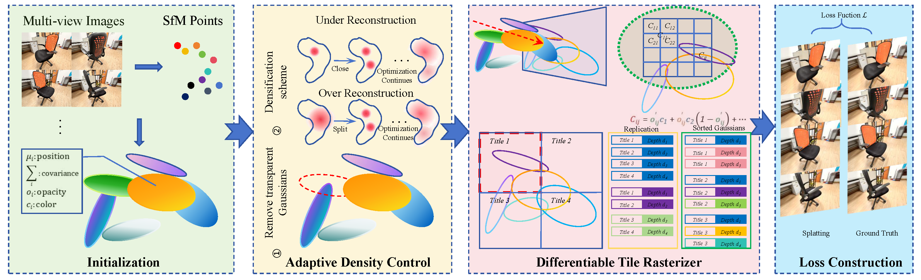
2. Background of 3DGS
3. Three-Dimensional Reconstruction and Rendering
3.1. Traditional 3D Reconstruction
3.1.1. Passive 3D Reconstruction
3.1.2. Active 3D Reconstruction
3.2. Deep Learning-Based 3D Reconstruction
3.2.1. Point Cloud-Based 3D Reconstruction
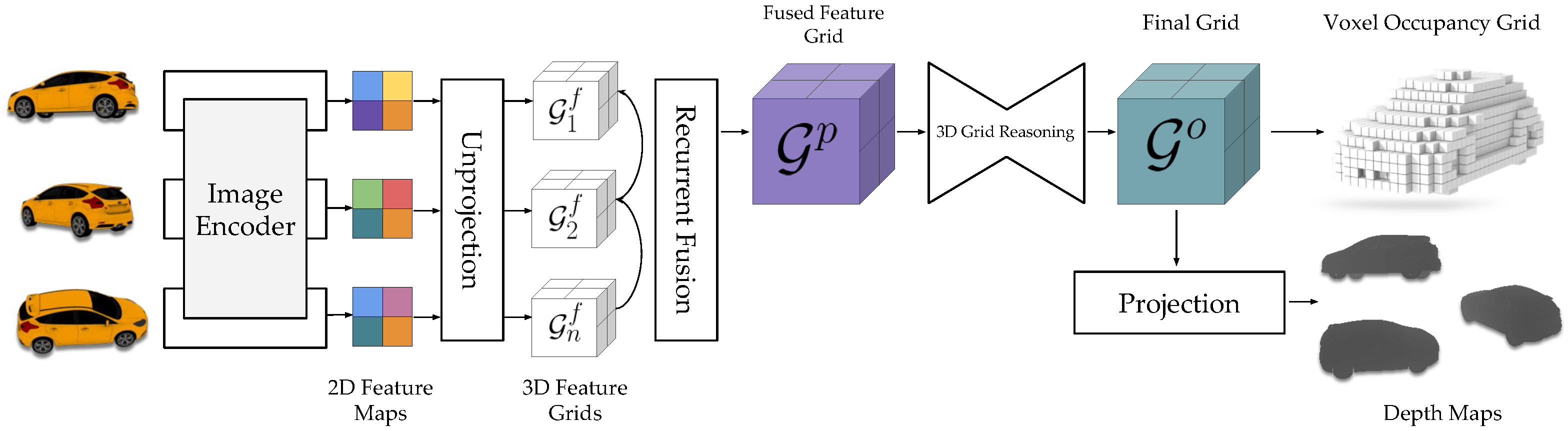
3.2.2. Voxel-Based 3D Reconstruction
3.2.3. Mesh-Based 3D Reconstruction
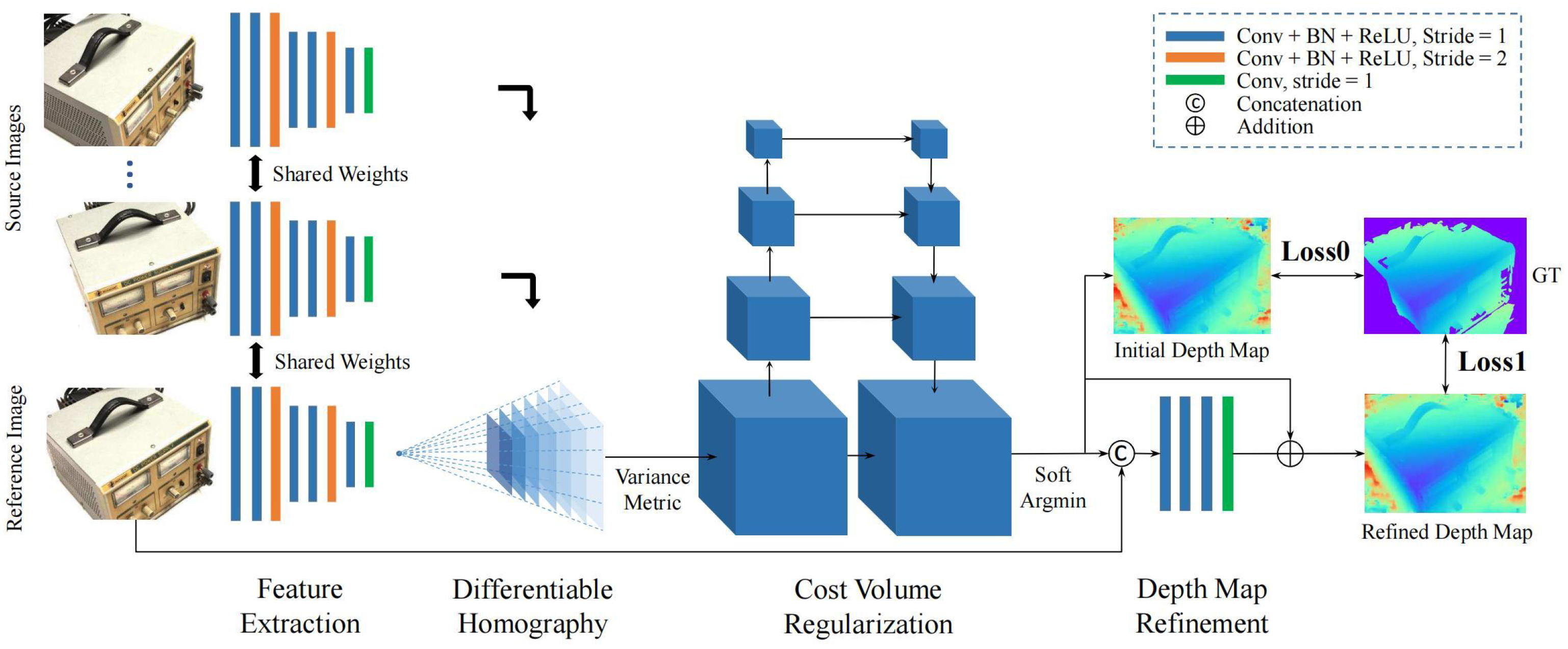
3.2.4. Depth Map-Based 3D Reconstruction
3.3. Three-Dimensional Rendering
3.3.1. Traditional 3D Rendering
3.3.2. Deep Learning-Based 3D Rendering
3.3.3. Gaussian Splatting-Based 3D Rendering
4. Datasets and Evaluation Metrics
4.1. Three-Dimensional Reconstruction
4.1.1. Datasets
4.1.2. Evaluation Metrics
4.2. Three-Dimensional Rendering
4.2.1. Datasets
4.2.2. Evaluation Metrics
5. Applications
6. Challenges and Future Trends
7. Conclusions
Author Contributions
Funding
Conflicts of Interest
References
- Schonberger, J.L.; Frahm, J.M. Structure-from-motion revisited. In Proceedings of the 2016 IEEE Conference on Computer Vision and Pattern Recognition (CVPR), Las Vegas, NV, USA, 27–30 June 2016; pp. 4104–4113. [Google Scholar]
- Zwicker, M.; Pfister, H.; Van Baar, J.; Gross, M. Surface splatting. In Proceedings of the 28th Annual Conference on Computer Graphics and Interactive Techniques, Los Angeles, CA, USA, 12–17 August 2001; pp. 371–378. [Google Scholar]
- Kopanas, G.; Philip, J.; Leimkühler, T.; Drettakis, G. Point-Based Neural Rendering with Per-View Optimization. In Computer Graphics Forum; Wiley Online Library: Hoboken, NJ, USA, 2021; Volume 40, pp. 29–43. [Google Scholar]
- Zwicker, M.; Pfister, H.; Van Baar, J.; Gross, M. EWA volume splatting. In Proceedings of the Proceedings Visualization, 2001. VIS ’01, San Diego, CA, USA, 21–26 October 2001; IEEE: New York, NY, USA, 2001; pp. 29–538. [Google Scholar]
- Botsch, M.; Kobbelt, L. High-quality point-based rendering on modern GPUs. In Proceedings of the 11th Pacific Conference on Computer Graphics and Applications, Canmore, AB, Canada, 8–10 October 2003; IEEE: New York, NY, USA, 2003; pp. 335–343. [Google Scholar]
- Rusinkiewicz, S.; Levoy, M. QSplat: A multiresolution point rendering system for large meshes. In Proceedings of the 27th Annual Conference on Computer Graphics and Interactive Techniques, New Orleans, LA, USA, 23–28 July 2000; pp. 343–352. [Google Scholar]
- Mildenhall, B.; Srinivasan, P.P.; Tancik, M.; Barron, J.T.; Ramamoorthi, R.; Ng, R. Nerf: Representing scenes as neural radiance fields for view synthesis. Commun. ACM 2021, 65, 99–106. [Google Scholar] [CrossRef]
- Yifan, W.; Serena, F.; Wu, S.; Öztireli, C.; Sorkine-Hornung, O. Differentiable surface splatting for point-based geometry processing. ACM Trans. Graph. (TOG) 2019, 38, 1–14. [Google Scholar] [CrossRef]
- Kerbl, B.; Kopanas, G.; Leimkühler, T.; Drettakis, G. 3D gaussian splatting for real-time radiance field rendering. ACM Trans. Graph. 2023, 42, 1–14. [Google Scholar] [CrossRef]
- Horn, B.K.P. Shape from Shading: A Method for Obtaining the Shape of a smooth Opaque Object from One View; Massachusetts Institute of Technology: Cambridge, MA, USA, 1970; Volume 232. [Google Scholar]
- Fan, J.; Chen, M.; Mo, J.; Wang, S.; Liang, Q. Variational formulation of a hybrid perspective shape from shading model. Vis. Comput. 2022, 38, 1469–1482. [Google Scholar] [CrossRef]
- Woodham, R.J. Photometric method for determining surface orientation from multiple images. Opt. Eng. 1980, 19, 139–144. [Google Scholar] [CrossRef]
- Shi, B.; Matsushita, Y.; Wei, Y.; Xu, C.; Tan, P. Self-calibrating photometric stereo. In Proceedings of the 2010 IEEE Computer Society Conference on Computer Vision and Pattern Recognition, San Francisco, CA, USA, 13–18 June 2010; IEEE: New York, NY, USA, 2010; pp. 1118–1125. [Google Scholar]
- Morris, N.J.; Kutulakos, K.N. Dynamic refraction stereo. IEEE Trans. Pattern Anal. Mach. Intell. 2011, 33, 1518–1531. [Google Scholar] [CrossRef]
- Shen, H.L.; Han, T.Q.; Li, C. Efficient photometric stereo using kernel regression. IEEE Trans. Image Process. 2016, 26, 439–451. [Google Scholar] [CrossRef]
- Sturm, P.; Triggs, B. A factorization based algorithm for multi-image projective structure and motion. In Proceedings of the Computer Vision—ECCV’96: 4th European Conference on Computer Vision, Cambridge, UK, 15–18 April 1996; Proceedings Volume II. Springer: Berlin/Heidelberg, Germany, 1996; pp. 709–720. [Google Scholar]
- Crandall, D.; Owens, A.; Snavely, N.; Huttenlocher, D. Discrete-continuous optimization for large-scale structure from motion. In Proceedings of the CVPR 2011, Colorado Springs, CO, USA, 20–25 June 2011; IEEE: New York, NY, USA, 2011; pp. 3001–3008. [Google Scholar]
- Moulon, P.; Monasse, P.; Marlet, R. Global fusion of relative motions for robust, accurate and scalable structure from motion. In Proceedings of the 2013 IEEE International Conference on Computer Vision, Sydney, NSW, Australia, 1–8 December 2013; pp. 3248–3255. [Google Scholar]
- Zhu, S.; Zhang, R.; Zhou, L.; Shen, T.; Fang, T.; Tan, P.; Quan, L. Very large-scale global sfm by distributed motion averaging. In Proceedings of the 2018 IEEE/CVF Conference on Computer Vision and Pattern Recognition, Salt Lake City, UT, USA, 18–23 June 2018; pp. 4568–4577. [Google Scholar]
- Wu, C. Towards linear-time incremental structure from motion. In Proceedings of the 2013 International Conference on 3D Vision—3DV 2013, Seattle, WA, USA, 29 June–1 July 2013; IEEE: New York, NY, USA, 2013; pp. 127–134. [Google Scholar]
- Wang, J.; Zhong, Y.; Dai, Y.; Birchfield, S.; Zhang, K.; Smolyanskiy, N.; Li, H. Deep two-view structure-from-motion revisited. In Proceedings of the 2021 IEEE/CVF Conference on Computer Vision and Pattern Recognition (CVPR), Nashville, TN, USA, 20–25 June 2021; pp. 8953–8962. [Google Scholar]
- Qu, Y.; Huang, J.; Zhang, X. Rapid 3D reconstruction for image sequence acquired from UAV camera. Sensors 2018, 18, 225. [Google Scholar] [CrossRef] [PubMed]
- Cui, H.; Shen, S.; Gao, W.; Liu, H.; Wang, Z. Efficient and robust large-scale structure-from-motion via track selection and camera prioritization. Isprs J. Photogramm. Remote. Sens. 2019, 156, 202–214. [Google Scholar] [CrossRef]
- Cui, H.; Gao, X.; Shen, S.; Hu, Z. HSfM: Hybrid structure-from-motion. In Proceedings of the 2017 IEEE Conference on Computer Vision and Pattern Recognition (CVPR), Honolulu, HI, USA, 21–26 July 2017; pp. 1212–1221. [Google Scholar]
- Zhu, S.; Shen, T.; Zhou, L.; Zhang, R.; Wang, J.; Fang, T.; Quan, L. Parallel structure from motion from local increment to global averaging. arXiv 2017, arXiv:1702.08601. [Google Scholar]
- Scharstein, D.; Szeliski, R. A taxonomy and evaluation of dense two-frame stereo correspondence algorithms. Int. J. Comput. Vis. 2002, 47, 7–42. [Google Scholar] [CrossRef]
- Huang, L.; Wu, G.; Liu, J.; Yang, S.; Cao, Q.; Ding, W.; Tang, W. Obstacle distance measurement based on binocular vision for high-voltage transmission lines using a cable inspection robot. Sci. Prog. 2020, 103, 0036850420936910. [Google Scholar] [CrossRef]
- Wei, M.; Shoulei, M.; Jianjian, B.; Chenbo, Y.; Donghui, C.; Hongfu, Y. Three-dimensional Reconstruction of Working Environment in Remote Control Excavator. In Proceedings of the 2020 5th International Conference on Mechanical, Control and Computer Engineering (ICMCCE), Harbin, China, 25–27 December 2020; IEEE: New York, NY, USA, 2020; pp. 98–103. [Google Scholar]
- Xu, T.; Chen, Z.; Jiang, Z.; Huang, J.; Gui, W. A real-time 3D measurement system for the blast furnace burden surface using high-temperature industrial endoscope. Sensors 2020, 20, 869. [Google Scholar] [CrossRef]
- Furukawa, Y.; Hernández, C. Multi-View Stereo: A Tutorial; Now Foundations and Trends: Norwell, MA, USA, 2015; Volume 9, pp. 1–148. [Google Scholar]
- Furukawa, Y.; Ponce, J. Accurate, dense, and robust multiview stereopsis. IEEE Trans. Pattern Anal. Mach. Intell. 2009, 32, 1362–1376. [Google Scholar] [CrossRef] [PubMed]
- Shen, S. Accurate multiple view 3D reconstruction using patch-based stereo for large-scale scenes. IEEE Trans. Image Process. 2013, 22, 1901–1914. [Google Scholar] [CrossRef]
- Zheng, E.; Dunn, E.; Jojic, V.; Frahm, J.M. Patchmatch based joint view selection and depthmap estimation. In Proceedings of the 2014 IEEE Conference on Computer Vision and Pattern Recognition, Columbus, OH, USA, 23–28 June 2014; pp. 1510–1517. [Google Scholar]
- Jashari, S.; Tukur, M.; Boraey, Y.; Alzubaidi, M.; Pintore, G.; Gobbetti, E.; Villanueva, A.J.; Schneider, J.; Fetais, N.; Agus, M. Evaluating AI-based static stereoscopic rendering of indoor panoramic scenes. In Proceedings of the STAG: Smart Tools and Applications in Graphics (2024), Verona, Italy, 14–15 November 2024. [Google Scholar]
- Pintore, G.; Jaspe-Villanueva, A.; Hadwiger, M.; Gobbetti, E.; Schneider, J.; Agus, M. PanoVerse: Automatic generation of stereoscopic environments from single indoor panoramic images for Metaverse applications. In Proceedings of the 28th International ACM Conference on 3D Web Technology, San Sebastian, Spain, 9–11 October 2023; pp. 1–10. [Google Scholar]
- Gunatilake, A.; Piyathilaka, L.; Kodagoda, S.; Barclay, S.; Vitanage, D. Real-time 3D profiling with RGB-D mapping in pipelines using stereo camera vision and structured IR laser ring. In Proceedings of the 2019 14th IEEE Conference on Industrial Electronics and Applications (ICIEA), Xi’an, China, 19–21 June 2019; IEEE: New York, NY, USA, 2019; pp. 916–921. [Google Scholar]
- Montusiewicz, J.; Miłosz, M.; Kęsik, J.; Żyła, K. Structured-light 3D scanning of exhibited historical clothing—A first-ever methodical trial and its results. Herit. Sci. 2021, 9, 74. [Google Scholar] [CrossRef]
- Chen, X.; Li, Q.; Wang, T.; Xue, T.; Pang, J. Gennbv: Generalizable next-best-view policy for active 3D reconstruction. In Proceedings of the 2024 IEEE/CVF Conference on Computer Vision and Pattern Recognition (CVPR), Seattle, WA, USA, 16–22 June 2024; pp. 16436–16445. [Google Scholar]
- Guðmundsson, S.Á.; Pardàs, M.; Casas, J.R.; Sveinsson, J.R.; Aanæs, H.; Larsen, R. Improved 3D reconstruction in smart-room environments using ToF imaging. Comput. Vis. Image Underst. 2010, 114, 1376–1384. [Google Scholar] [CrossRef]
- Hoegg, T.; Lefloch, D.; Kolb, A. Time-of-Flight camera based 3D point cloud reconstruction of a car. Comput. Ind. 2013, 64, 1099–1114. [Google Scholar] [CrossRef]
- Li, L.; Liu, H.; Xu, Y.; Zheng, Y. Measurement linearity and accuracy optimization for time-of-flight range imaging cameras. In Proceedings of the 2020 IEEE 4th Information Technology, Networking, Electronic and Automation Control Conference (ITNEC), Chongqing, China, 12–14 June 2020; IEEE: New York, NY, USA, 2020; Volume 1, pp. 520–524. [Google Scholar]
- Fitrah, P.A.; Ramadhani, C.R.; Rahmi, D.A.; Harisna, N. Use of LiDAR in Topographic Map Mapping or Surface Mapping. J. Front. Res. Sci. Eng. 2024, 2, 19–25. [Google Scholar]
- Liao, G.; Li, J.; Ye, X. VLM2Scene: Self-supervised image-text-LiDAR learning with foundation models for autonomous driving scene understanding. In Proceedings of the AAAI Conference on Artificial Intelligence, Vancouver, BC, Canada, 20–27 February 2024; Volume 38, pp. 3351–3359. [Google Scholar]
- Schwalbe, E.; Maas, H.G.; Seidel, F. 3D building model generation from airborne laser scanner data using 2D GIS data and orthogonal point cloud projections. Proc. ISPRS WG III/3 III/4 2005, 3, 12–14. [Google Scholar]
- Feng, H.; Chen, Y.; Luo, Z.; Sun, W.; Li, W.; Li, J. Automated extraction of building instances from dual-channel airborne LiDAR point clouds. Int. J. Appl. Earth Obs. Geoinf. 2022, 114, 103042. [Google Scholar] [CrossRef]
- Zhong, X.; Pan, Y.; Stachniss, C.; Behley, J. 3D LiDAR Mapping in Dynamic Environments Using a 4D Implicit Neural Representation. In Proceedings of the 2024 IEEE/CVF Conference on Computer Vision and Pattern Recognition (CVPR), Seattle, WA, USA, 16–22 June 2024; pp. 15417–15427. [Google Scholar]
- Tukur, M.; Boraey, Y.; Jashari, S.; Villanueva, A.J.; Shah, U.; Al-Zubaidi, M.; Pintore, G.; Gobbetti, E.; Schneider, J.; Agus, M.; et al. Virtual Staging Technologies for the Metaverse. In Proceedings of the 2024 2nd International Conference on Intelligent Metaverse Technologies & Applications (iMETA), Dubai, United Arab Emirates, 26–29 November 2024; IEEE: New York, NY, USA, 2024; pp. 206–213. [Google Scholar]
- Seitz, S.M.; Curless, B.; Diebel, J.; Scharstein, D.; Szeliski, R. A comparison and evaluation of multi-view stereo reconstruction algorithms. In Proceedings of the 2006 IEEE Computer Society Conference on Computer Vision and Pattern Recognition (CVPR’06), New York, NY, USA, 17–22 June 2006; IEEE: New York, NY, USA, 2006; Volume 1, pp. 519–528. [Google Scholar]
- Yao, Y.; Luo, Z.; Li, S.; Fang, T.; Quan, L. Mvsnet: Depth inference for unstructured multi-view stereo. In Proceedings of the European Conference on Computer Vision (ECCV), Munich, Germany, 8–14 September 2018; pp. 767–783. [Google Scholar]
- Chen, R.; Han, S.; Xu, J.; Su, H. Point-based multi-view stereo network. In Proceedings of the 2019 IEEE/CVF International Conference on Computer Vision (ICCV), Seoul, Republic of Korea, 27 October–2 November 2019; pp. 1538–1547. [Google Scholar]
- Huang, B.; Yi, H.; Huang, C.; He, Y.; Liu, J.; Liu, X. M3VSNet: Unsupervised multi-metric multi-view stereo network. In Proceedings of the 2021 IEEE International Conference on Image Processing (ICIP), Anchorage, AK, USA, 19–22 September 2021; IEEE: New York, NY, USA, 2021; pp. 3163–3167. [Google Scholar]
- Nichol, A.; Jun, H.; Dhariwal, P.; Mishkin, P.; Chen, M. Point-e: A system for generating 3D point clouds from complex prompts. arXiv 2022, arXiv:2212.08751. [Google Scholar]
- Li, S.; Gao, P.; Tan, X.; Wei, M. Proxyformer: Proxy alignment assisted point cloud completion with missing part sensitive transformer. In Proceedings of the 2023 IEEE/CVF Conference on Computer Vision and Pattern Recognition (CVPR), Vancouver, BC, Canada, 17–24 June 2023; pp. 9466–9475. [Google Scholar]
- Zhang, Y.; Zhu, J.; Lin, L. Multi-view stereo representation revist: Region-aware mvsnet. In Proceedings of the 2023 IEEE/CVF Conference on Computer Vision and Pattern Recognition (CVPR), Vancouver, BC, Canada, 17–24 June 2023; pp. 17376–17385. [Google Scholar]
- Koch, S.; Hermosilla, P.; Vaskevicius, N.; Colosi, M.; Ropinski, T. Sgrec3d: Self-supervised 3D scene graph learning via object-level scene reconstruction. In Proceedings of the 2024 IEEE/CVF Winter Conference on Applications of Computer Vision (WACV), Waikoloa, HI, USA, 3–8 January 2024; pp. 3404–3414. [Google Scholar]
- Ji, M.; Gall, J.; Zheng, H.; Liu, Y.; Fang, L. Surfacenet: An end-to-end 3D neural network for multiview stereopsis. In Proceedings of the 2017 IEEE International Conference on Computer Vision (ICCV), Venice, Italy, 22–29 October 2017; pp. 2307–2315. [Google Scholar]
- Kar, A.; Häne, C.; Malik, J. Learning a multi-view stereo machine. Adv. Neural Inf. Process. Syst. 2017, 30, 364–375. [Google Scholar]
- Liu, S.; Giles, L.; Ororbia, A. Learning a hierarchical latent-variable model of 3D shapes. In Proceedings of the 2018 International Conference on 3D Vision (3DV), Verona, Italy, 5–8 September 2018; IEEE: New York, NY, USA, 2018; pp. 542–551. [Google Scholar]
- Wang, D.; Cui, X.; Chen, X.; Zou, Z.; Shi, T.; Salcudean, S.; Wang, Z.J.; Ward, R. Multi-view 3D reconstruction with transformers. In Proceedings of the 2021 IEEE/CVF International Conference on Computer Vision (ICCV), Montreal, QC, Canada, 10–17 October 2021; pp. 5722–5731. [Google Scholar]
- Schwarz, K.; Sauer, A.; Niemeyer, M.; Liao, Y.; Geiger, A. Voxgraf: Fast 3D-aware image synthesis with sparse voxel grids. Adv. Neural Inf. Process. Syst. 2022, 35, 33999–34011. [Google Scholar]
- Wang, Y.; Guan, T.; Chen, Z.; Luo, Y.; Luo, K.; Ju, L. Mesh-guided multi-view stereo with pyramid architecture. In Proceedings of the 2020 IEEE/CVF Conference on Computer Vision and Pattern Recognition (CVPR), Seattle, WA, USA, 13–19 June 2020; pp. 2039–2048. [Google Scholar]
- Yuan, Y.; Tang, J.; Zou, Z. Vanet: A view attention guided network for 3D reconstruction from single and multi-view images. In Proceedings of the 2021 IEEE International Conference on Multimedia and Expo (ICME), Shenzhen, China, 5–9 July 2021; IEEE: New York, NY, USA, 2021; pp. 1–6. [Google Scholar]
- Ju, J.; Tseng, C.W.; Bailo, O.; Dikov, G.; Ghafoorian, M. Dg-recon: Depth-guided neural 3d scene reconstruction. In Proceedings of the 2023 IEEE/CVF International Conference on Computer Vision (ICCV), Paris, France, 1–6 October 2023; pp. 18184–18194. [Google Scholar]
- Wang, Z.; Zhou, S.; Park, J.J.; Paschalidou, D.; You, S.; Wetzstein, G.; Guibas, L.; Kadambi, A. Alto: Alternating latent topologies for implicit 3D reconstruction. In Proceedings of the 2023 IEEE/CVF Conference on Computer Vision and Pattern Recognition (CVPR), Vancouver, BC, Canada, 17–24 June 2023; pp. 259–270. [Google Scholar]
- Dogaru, A.; Özer, M.; Egger, B. Generalizable 3D scene reconstruction via divide and conquer from a single view. arXiv 2024, arXiv:arXiv:2404.03421. [Google Scholar]
- Huang, P.H.; Matzen, K.; Kopf, J.; Ahuja, N.; Huang, J.B. Deepmvs: Learning multi-view stereopsis. In Proceedings of the 2018 IEEE/CVF Conference on Computer Vision and Pattern Recognition, Salt Lake City, UT, USA, 18–23 June 2018; pp. 2821–2830. [Google Scholar]
- Yi, H.; Wei, Z.; Ding, M.; Zhang, R.; Chen, Y.; Wang, G.; Tai, Y.W. Pyramid multi-view stereo net with self-adaptive view aggregation. In Proceedings of the Computer Vision–ECCV 2020: 16th European Conference, Glasgow, UK, 23–28 August 2020; Proceedings, Part IX 16. Springer: Berlin/Heidelberg, Germany, 2020; pp. 766–782. [Google Scholar]
- Zhang, Z.; Peng, R.; Hu, Y.; Wang, R. Geomvsnet: Learning multi-view stereo with geometry perception. In Proceedings of the 2023 IEEE/CVF Conference on Computer Vision and Pattern Recognition (CVPR), Vancouver, BC, Canada, 17–24 June 2023; pp. 21508–21518. [Google Scholar]
- Dib, A.; Bharaj, G.; Ahn, J.; Thébault, C.; Gosselin, P.; Romeo, M.; Chevallier, L. Practical face reconstruction via differentiable ray tracing. In Computer Graphics Forum; Wiley Online Library: Hoboken, NJ, USA, 2021; Volume 40, pp. 153–164. [Google Scholar]
- Zhang, Y.; Orth, A.; England, D.; Sussman, B. Ray tracing with quantum correlated photons to image a three-dimensional scene. Phys. Rev. A 2022, 105, L011701. [Google Scholar] [CrossRef]
- Ma, J.; Liu, M.; Ahmedt-Aristizabal, D.; Nguyen, C. HashPoint: Accelerated Point Searching and Sampling for Neural Rendering. In Proceedings of the 2024 IEEE/CVF Conference on Computer Vision and Pattern Recognition (CVPR), Seattle, WA, USA, 16–22 June 2024; pp. 4462–4472. [Google Scholar]
- Anciukevičius, T.; Xu, Z.; Fisher, M.; Henderson, P.; Bilen, H.; Mitra, N.J.; Guerrero, P. Renderdiffusion: Image diffusion for 3D reconstruction, inpainting and generation. In Proceedings of the 2023 IEEE/CVF Conference on Computer Vision and Pattern Recognition (CVPR), Vancouver, BC, Canada, 17–24 June 2023; pp. 12608–12618. [Google Scholar]
- Zhou, Z.; Tulsiani, S. Sparsefusion: Distilling view-conditioned diffusion for 3D reconstruction. In Proceedings of the 2023 IEEE/CVF Conference on Computer Vision and Pattern Recognition (CVPR), Vancouver, BC, Canada, 17–24 June 2023; pp. 12588–12597. [Google Scholar]
- An, S.; Xu, H.; Shi, Y.; Song, G.; Ogras, U.Y.; Luo, L. Panohead: Geometry-aware 3D full-head synthesis in 360deg. In Proceedings of the 2023 IEEE/CVF Conference on Computer Vision and Pattern Recognition (CVPR), Vancouver, BC, Canada, 17–24 June 2023; pp. 20950–20959. [Google Scholar]
- Mirzaei, A.; Aumentado-Armstrong, T.; Derpanis, K.G.; Kelly, J.; Brubaker, M.A.; Gilitschenski, I.; Levinshtein, A. Spin-nerf: Multiview segmentation and perceptual inpainting with neural radiance fields. In Proceedings of the 2023 IEEE/CVF Conference on Computer Vision and Pattern Recognition (CVPR), Vancouver, BC, Canada, 17–24 June 2023; pp. 20669–20679. [Google Scholar]
- Bian, W.; Wang, Z.; Li, K.; Bian, J.W.; Prisacariu, V.A. Nope-nerf: Optimising neural radiance field with no pose prior. In Proceedings of the 2023 IEEE/CVF Conference on Computer Vision and Pattern Recognition (CVPR), Vancouver, BC, Canada, 17–24 June 2023; pp. 4160–4169. [Google Scholar]
- Wynn, J.; Turmukhambetov, D. Diffusionerf: Regularizing neural radiance fields with denoising diffusion models. In Proceedings of the 2023 IEEE/CVF Conference on Computer Vision and Pattern Recognition (CVPR), Vancouver, BC, Canada, 17–24 June 2023; pp. 4180–4189. [Google Scholar]
- Wu, G.; Yi, T.; Fang, J.; Xie, L.; Zhang, X.; Wei, W.; Liu, W.; Tian, Q.; Wang, X. 4d gaussian splatting for real-time dynamic scene rendering. In Proceedings of the 2024 IEEE/CVF Conference on Computer Vision and Pattern Recognition (CVPR), Seattle, WA, USA, 16–22 June 2024; pp. 20310–20320. [Google Scholar]
- Sless, L.; El Shlomo, B.; Cohen, G.; Oron, S. Road scene understanding by occupancy grid learning from sparse radar clusters using semantic segmentation. In Proceedings of the 2019 IEEE/CVF International Conference on Computer Vision Workshop (ICCVW), Seoul, Republic of Korea, 27–28 October 2019; pp. 867–875. [Google Scholar]
- Zhao, P.; Lu, C.X.; Wang, J.; Chen, C.; Wang, W.; Trigoni, N.; Markham, A. Human tracking and identification through a millimeter wave radar. Ad. Hoc. Networks 2021, 116, 102475. [Google Scholar] [CrossRef]
- Zhang, K.; Bi, S.; Tan, H.; Xiangli, Y.; Zhao, N.; Sunkavalli, K.; Xu, Z. Gs-lrm: Large reconstruction model for 3D gaussian splatting. In European Conference on Computer Vision; Springer: Berlin/Heidelberg, Germany, 2024; pp. 1–19. [Google Scholar]
- Chen, C.; Fragonara, L.Z.; Tsourdos, A. RoIFusion: 3D object detection from LiDAR and vision. IEEE Access 2021, 9, 51710–51721. [Google Scholar] [CrossRef]
- Gao, J.; Gu, C.; Lin, Y.; Li, Z.; Zhu, H.; Cao, X.; Zhang, L.; Yao, Y. Relightable 3D gaussians: Realistic point cloud relighting with brdf decomposition and ray tracing. In European Conference on Computer Vision; Springer: Berlin/Heidelberg, Germany, 2024; pp. 73–89. [Google Scholar]
- Lee, B.; Lee, H.; Sun, X.; Ali, U.; Park, E. Deblurring 3D gaussian splatting. In European Conference on Computer Vision; Springer: Berlin/Heidelberg, Germany, 2024; pp. 127–143. [Google Scholar]
- Liu, Y.; Luo, C.; Fan, L.; Wang, N.; Peng, J.; Zhang, Z. Citygaussian: Real-time high-quality large-scale scene rendering with gaussians. In European Conference on Computer Vision; Springer: Berlin/Heidelberg, Germany, 2024; pp. 265–282. [Google Scholar]
- Yu, Z.; Chen, A.; Huang, B.; Sattler, T.; Geiger, A. Mip-splatting: Alias-free 3D gaussian splatting. In Proceedings of the 2024 IEEE/CVF Conference on Computer Vision and Pattern Recognition (CVPR), Seattle, WA, USA, 16–22 June 2024; pp. 19447–19456. [Google Scholar]
- Sun, L.C.; Bhatt, N.P.; Liu, J.C.; Fan, Z.; Wang, Z.; Humphreys, T.E.; Topcu, U. Mm3dgs slam: Multi-modal 3D gaussian splatting for slam using vision, depth, and inertial measurements. In Proceedings of the 2024 IEEE/RSJ International Conference on Intelligent Robots and Systems (IROS), Abu Dhabi, United Arab Emirates, 14–18 October 2024; IEEE: New York, NY, USA, 2024; pp. 10159–10166. [Google Scholar]
- Sun, J.; Jiao, H.; Li, G.; Zhang, Z.; Zhao, L.; Xing, W. 3dgstream: On-the-fly training of 3D gaussians for efficient streaming of photo-realistic free-viewpoint videos. In Proceedings of the 2024 IEEE/CVF Conference on Computer Vision and Pattern Recognition (CVPR), Seattle, WA, USA, 16–22 June 2024; pp. 20675–20685. [Google Scholar]
- Liang, Z.; Zhang, Q.; Feng, Y.; Shan, Y.; Jia, K. Gs-ir: 3D gaussian splatting for inverse rendering. In Proceedings of the 2024 IEEE/CVF Conference on Computer Vision and Pattern Recognition (CVPR), Seattle, WA, USA, 16–22 June 2024; pp. 21644–21653. [Google Scholar]
- Guédon, A.; Lepetit, V. Sugar: Surface-aligned gaussian splatting for efficient 3D mesh reconstruction and high-quality mesh rendering. In Proceedings of the 2024 IEEE/CVF Conference on Computer Vision and Pattern Recognition (CVPR), Seattle, WA, USA, 16–22 June 2024; pp. 5354–5363. [Google Scholar]
- Chen, Y.; Lee, G.H. Dogaussian: Distributed-oriented gaussian splatting for large-scale 3D reconstruction via gaussian consensus. arXiv 2024, arXiv:2405.13943. [Google Scholar]
- Zielonka, W.; Bagautdinov, T.; Saito, S.; Zollhöfer, M.; Thies, J.; Romero, J. Drivable 3D gaussian avatars. arXiv 2023, arXiv:2311.08581. [Google Scholar]
- Duisterhof, B.P.; Mandi, Z.; Yao, Y.; Liu, J.W.; Shou, M.Z.; Song, S.; Ichnowski, J. Md-splatting: Learning metric deformation from 4D gaussians in highly deformable scenes. arXiv 2023, arXiv:2312.00583. [Google Scholar]
- Wang, J.; Fang, J.; Zhang, X.; Xie, L.; Tian, Q. Gaussianeditor: Editing 3D gaussians delicately with text instructions. In Proceedings of the 2024 IEEE/CVF Conference on Computer Vision and Pattern Recognition (CVPR), Seattle, WA, USA, 16–22 June 2024; pp. 20902–20911. [Google Scholar]
- Sturm, J.; Engelhard, N.; Endres, F.; Burgard, W.; Cremers, D. A benchmark for the evaluation of RGB-D SLAM systems. In Proceedings of the 2012 IEEE/RSJ International Conference on Intelligent Robots and Systems, Vilamoura-Algarve, Portugal, 7–12 October 2012; IEEE: New York, NY, USA, 2012; pp. 573–580. [Google Scholar]
- Geiger, A.; Lenz, P.; Stiller, C.; Urtasun, R. Vision meets robotics: The kitti dataset. Int. J. Robot. Res. 2013, 32, 1231–1237. [Google Scholar] [CrossRef]
- Xiao, J.; Owens, A.; Torralba, A. Sun3d: A database of big spaces reconstructed using sfm and object labels. In Proceedings of the 2013 IEEE International Conference on Computer Vision, Sydney, NSW, Australia, 1–8 December 2013; pp. 1625–1632. [Google Scholar]
- Chang, A.X.; Funkhouser, T.; Guibas, L.; Hanrahan, P.; Huang, Q.; Li, Z.; Savarese, S.; Savva, M.; Song, S.; Su, H.; et al. Shapenet: An information-rich 3D model repository. arXiv 2015, arXiv:1512.03012. [Google Scholar]
- Wu, Z.; Song, S.; Khosla, A.; Yu, F.; Zhang, L.; Tang, X.; Xiao, J. 3D shapenets: A deep representation for volumetric shapes. In Proceedings of the 2015 IEEE Conference on Computer Vision and Pattern Recognition (CVPR), Boston, MA, USA, 7–12 June 2015; pp. 1912–1920. [Google Scholar]
- Aanæs, H.; Jensen, R.R.; Vogiatzis, G.; Tola, E.; Dahl, A.B. Large-scale data for multiple-view stereopsis. Int. J. Comput. Vis. 2016, 120, 153–168. [Google Scholar] [CrossRef]
- Schops, T.; Schonberger, J.L.; Galliani, S.; Sattler, T.; Schindler, K.; Pollefeys, M.; Geiger, A. A multi-view stereo benchmark with high-resolution images and multi-camera videos. In Proceedings of the 2017 IEEE Conference on Computer Vision and Pattern Recognition (CVPR), Honolulu, HI, USA, 21–26 July 2017; pp. 3260–3269. [Google Scholar]
- Knapitsch, A.; Park, J.; Zhou, Q.Y.; Koltun, V. Tanks and temples: Benchmarking large-scale scene reconstruction. ACM Trans. Graph. (ToG) 2017, 36, 1–13. [Google Scholar] [CrossRef]
- Dai, A.; Chang, A.X.; Savva, M.; Halber, M.; Funkhouser, T.; Nießner, M. Scannet: Richly-annotated 3D reconstructions of indoor scenes. In Proceedings of the 2017 IEEE Conference on Computer Vision and Pattern Recognition (CVPR), Honolulu, HI, USA, 21–26 July 2017; pp. 5828–5839. [Google Scholar]
- Mildenhall, B.; Srinivasan, P.P.; Ortiz-Cayon, R.; Kalantari, N.K.; Ramamoorthi, R.; Ng, R.; Kar, A. Local light field fusion: Practical view synthesis with prescriptive sampling guidelines. ACM Trans. Graph. (ToG) 2019, 38, 1–14. [Google Scholar] [CrossRef]
- Hedman, P.; Philip, J.; Price, T.; Frahm, J.M.; Drettakis, G.; Brostow, G. Deep blending for free-viewpoint image-based rendering. ACM Trans. Graph. (ToG) 2018, 37, 1–15. [Google Scholar] [CrossRef]
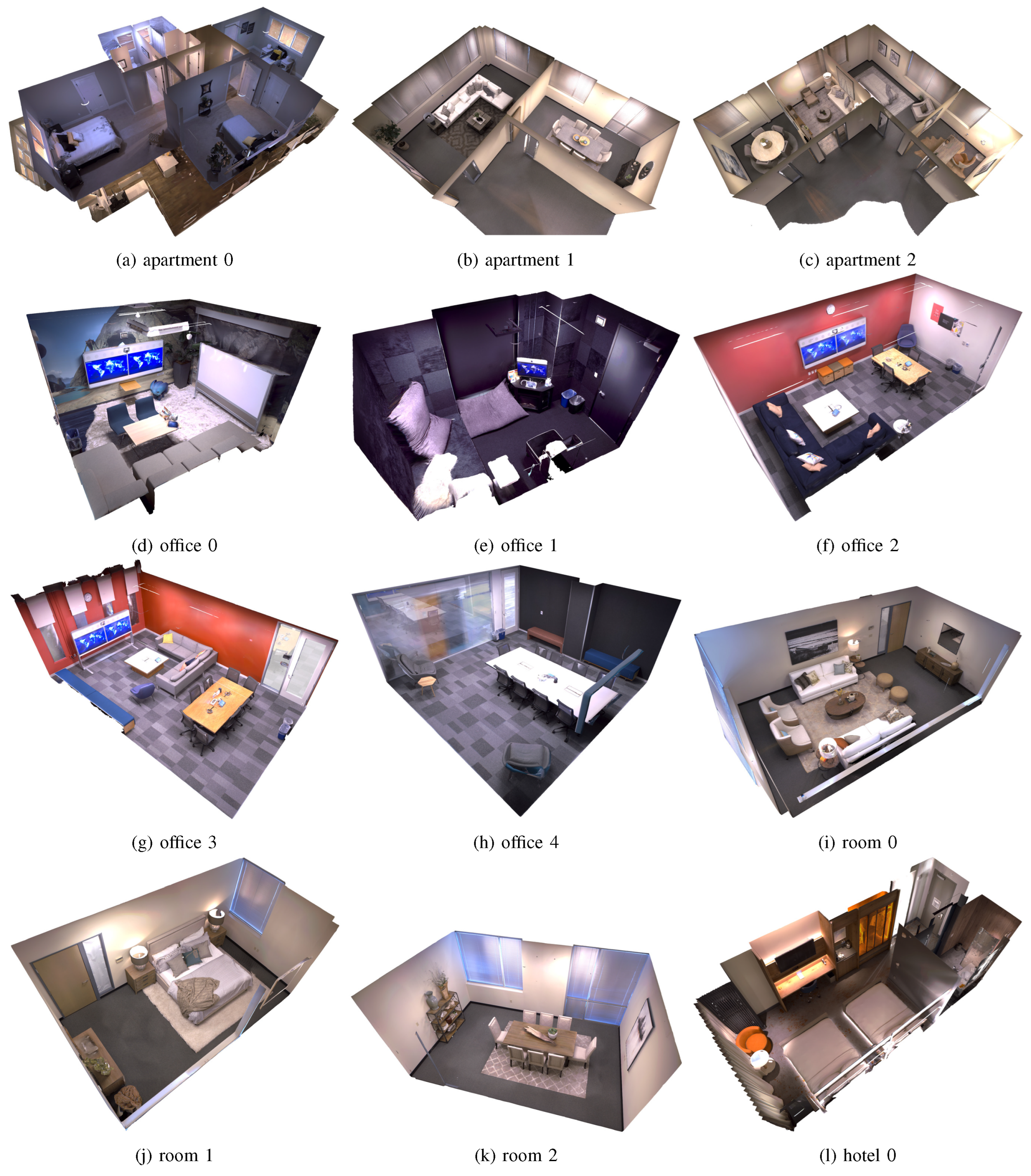
- Straub, J.; Whelan, T.; Ma, L.; Chen, Y.; Wijmans, E.; Green, S.; Engel, J.J.; Mur-Artal, R.; Ren, C.; Verma, S.; et al. The replica dataset: A digital replica of indoor spaces. arXiv 2019, arXiv:1906.05797. [Google Scholar]
- Yao, Y.; Luo, Z.; Li, S.; Zhang, J.; Ren, Y.; Zhou, L.; Fang, T.; Quan, L. Blendedmvs: A large-scale dataset for generalized multi-view stereo networks. In Proceedings of the 2020 IEEE/CVF Conference on Computer Vision and Pattern Recognition (CVPR), Seattle, WA, USA, 13–19 June 2020; pp. 1790–1799. [Google Scholar]
- Barron, J.T.; Mildenhall, B.; Verbin, D.; Srinivasan, P.P.; Hedman, P. Mip-nerf 360: Unbounded anti-aliased neural radiance fields. In Proceedings of the 2022 IEEE/CVF Conference on Computer Vision and Pattern Recognition (CVPR), New Orleans, LA, USA, 18–24 June 2022; pp. 5470–5479. [Google Scholar]
- Xiangli, Y.; Xu, L.; Pan, X.; Zhao, N.; Rao, A.; Theobalt, C.; Dai, B.; Lin, D. Bungeenerf: Progressive neural radiance field for extreme multi-scale scene rendering. In European Conference on Computer Vision; Springer: Berlin/Heidelberg, Germany, 2022; pp. 106–122. [Google Scholar]
- Lin, L.; Liu, Y.; Hu, Y.; Yan, X.; Xie, K.; Huang, H. Capturing, reconstructing, and simulating: The urbanscene3d dataset. In European Conference on Computer Vision; Springer: Berlin/Heidelberg, Germany, 2022; pp. 93–109. [Google Scholar]
- Jin, H.; Liu, I.; Xu, P.; Zhang, X.; Han, S.; Bi, S.; Zhou, X.; Xu, Z.; Su, H. Tensoir: Tensorial inverse rendering. In Proceedings of the 2023 IEEE/CVF Conference on Computer Vision and Pattern Recognition (CVPR), Vancouver, BC, Canada, 17–24 June 2023; pp. 165–174. [Google Scholar]
- Wang, Z.; Bovik, A.C.; Sheikh, H.R.; Simoncelli, E.P. Image quality assessment: From error visibility to structural similarity. IEEE Trans. Image Process. 2004, 13, 600–612. [Google Scholar] [CrossRef]
- Huang, L.; Bai, J.; Guo, J.; Li, Y.; Guo, Y. On the error analysis of 3D gaussian splatting and an optimal projection strategy. In European Conference on Computer Vision; Springer: Berlin/Heidelberg, Germany, 2024; pp. 247–263. [Google Scholar]
- Navaneet, K.; Meibodi, K.P.; Koohpayegani, S.A.; Pirsiavash, H. Compact3d: Compressing gaussian splat radiance field models with vector quantization. arXiv 2023, arXiv:2311.18159. [Google Scholar]
- Girish, S.; Gupta, K.; Shrivastava, A. Eagles: Efficient accelerated 3D gaussians with lightweight encodings. In European Conference on Computer Vision; Springer: Berlin/Heidelberg, Germany, 2024; pp. 54–71. [Google Scholar]
- Cheng, K.; Long, X.; Yang, K.; Yao, Y.; Yin, W.; Ma, Y.; Wang, W.; Chen, X. Gaussianpro: 3d gaussian splatting with progressive propagation. In Proceedings of the Forty-First International Conference on Machine Learning, Vienna, Austria, 21–27 July 2024. [Google Scholar]
- Lee, J.C.; Rho, D.; Sun, X.; Ko, J.H.; Park, E. Compact 3D gaussian representation for radiance field. In Proceedings of the 2024 IEEE/CVF Conference on Computer Vision and Pattern Recognition (CVPR), Seattle, WA, USA, 16–22 June 2024; pp. 21719–21728. [Google Scholar]
- Han, Y.; Yu, T.; Yu, X.; Xu, D.; Zheng, B.; Dai, Z.; Yang, C.; Wang, Y.; Dai, Q. Super-NeRF: View-consistent detail generation for NeRF super-resolution. IEEE Trans. Vis. Comput. Graph. 2024, 1–14. [Google Scholar] [CrossRef] [PubMed]
- Li, D.; Huang, S.S.; Huang, H. MPGS: Multi-plane Gaussian Splatting for Compact Scenes Rendering. IEEE Trans. Vis. Comput. Graph. 2025, 31, 3256–3266. [Google Scholar] [CrossRef] [PubMed]
- Dai, P.; Xu, J.; Xie, W.; Liu, X.; Wang, H.; Xu, W. High-quality surface reconstruction using gaussian surfels. In ACM SIGGRAPH 2024 Conference Papers; Association for Computing: New York, NY, USA, 2024; pp. 1–11. [Google Scholar]
- Yu, Z.; Sattler, T.; Geiger, A. Gaussian opacity fields: Efficient adaptive surface reconstruction in unbounded scenes. ACM Trans. Graph. (TOG) 2024, 43, 1–13. [Google Scholar] [CrossRef]


| Year | Dataset | Data Composition | Description | Tasks |
|---|---|---|---|---|
| 2012 | TUM RGB-D | 39 sequences: RGB/depth images, camera pose | Indoor scenes from RGB-D camera | Quantitative evaluation |
| 2013 | KITTI | 14,999 images: RGB/grayscale images, point clouds, GPS/IMU/calibration data, annotations | Large-scale outdoor scenes from cameras, Velodyne HDL-64E LiDAR and GPS/IMU | Recognition, segmentation, and optical flow estimation |
| 2013 | SUN3D | 415 scenes: depth images, point clouds, camera poses, semantic segmentation | Multiview indoor scenes from RGB-D sensors | Reconstruction and understanding |
| 2015 | ShapeNet | 3M models: 3D CAD models | 3D model categories | Recognition, generation, and classification |
| 2015 | ModelNet | 127,915 models: 3D CAD models | 3D model categories | Classification |
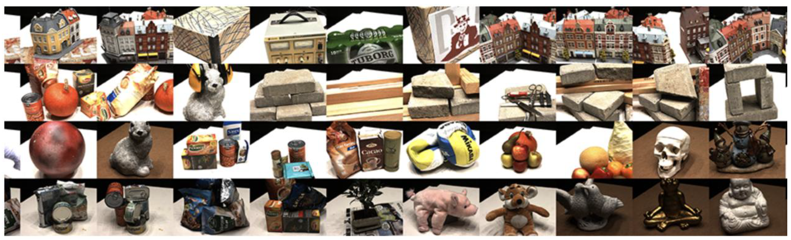
| 2016 | DTU | 128 scenes: RGB/depth images, point clouds, camera parameter | Multiview stereo depth indoor dataset from industrial robot | Reconstruction, depth estimation, and visual SLAM |
| 2017 | ETH3D | 35 scenes: RGB images | Indoor/out scenes from DSLR cameras | Depth estimation and reconstruction |
| 2017 | Tanks and Temples | 14 scenes: point clouds, video sequences | Indoor/outdoor 3D reconstruction dataset from cameras and LiDAR | Reconstruction |
| 2017 | ScanNet | 1513 scenes: RGB-D videos, point clouds | Indoor/outdoor scenes with semantic images from RGB-D cameras | Reconstruction, recognition, and understanding |
| 2019 | LLFF | 24 scenes: RGB images, pose estimation data | Light field indoor data from multiview smartphone cameras | View synthesis and reconstruction |
| 2022 | Mip-NeRF 360 | 9 scenes including 5 outdoor and 4 indoor | Multiview images with depth information with resolution of pixels | Unbounded scenes (camera facing any direction, content distributed at any distance) |
| 2024 | UT-MM | 8 scenes: RGB/depth images, LiDAR, IMU, etc. | Multimodal indoor/outdoor scenes from mobile robot | Multimodal learning and cross-modal retrieval |
| Methods | Datasets | PSNR ↑ | SSIM ↑ | LPIPS ↓ | FPS ↑ |
|---|---|---|---|---|---|
| 3DGS [9] | Tanks and Temples | 23.14 | 0.841 | 0.183 | 154 |
| 3DGS (OPS) [113] | Tanks and Temples | 26.44 | 0.872 | 0.214 | – |
| NeRF (Mip-NeRF 360) [108] | Tanks and Temples | 22.22 | 0.760 | 0.260 | 0.14 |
| 3DGS [9] | Mip-NeRF 360 | 27.21 | 0.815 | 0.214 | 134 |
| 3DGS (OPS) [113] | Mip-NeRF 360 | 27.48 | 0.821 | 0.209 | – |
| 3DGS (Compact3D) [114] | Mip-NeRF 360 | 27.16 | 0.808 | 0.228 | – |
| 3DGS (EAGLES) [115] | Mip-NeRF 360 | 27.15 | 0.810 | 0.240 | – |
| 3DGS (GsPro) [116] | Mip-NeRF 360 | 27.92 | 0.825 | 0.208 | – |
| 3DGS (C3DGS) [117] | Mip-NeRF 360 | 27.08 | 0.798 | 0.247 | – |
| NeRF (Mip-NeRF 360) [108] | Mip-NeRF 360 | 27.69 | 0.790 | 0.240 | 0.06 |
| 3DGS [9] | LLFF | 24.37 | 0.822 | 0.262 | 445 |
| NeRF [7] | LLFF | 26.50 | 0.811 | 0.250 | – |
| NeRF (Super-NeRF) [118] | LLFF | 27.75 | 0.863 | 0.087 | – |
| 3DGS (MPGS) [119] | LLFF | 27.15 | 0.868 | 0.202 | 469 |
| 3DGS (GSPro) [116] | LLFF | 26.83 | 0.869 | 0.196 | 199 |
| 3DGS (SurfelGS) [120] | LLFF | 26.73 | 0.869 | 0.190 | 107 |
| 3DGS (GoF) [121] | LLFF | 26.93 | 0.867 | 0.182 | 388 |
| Application Domain | Representative Methods | Strengths | Challenges |
|---|---|---|---|
| Real-Time Rendering and View Synthesis | 3DGS [9], EAGLES [115], MPGS [119] | Real-time performance, high-quality novel view synthesis, compatible with rasterization pipelines | Multi-scale rendering artifacts, high memory consumption |
| Autonomous Driving and Dynamic Scenes | GaussianPro [116], C3DGS [117], NeRF [7] | Dynamic object modeling, real-time LiDAR data fusion, strong cross-dataset generalization | Difficulty handling motion blur, high computational load in large-scale scenes |
| Surface Reconstruction and Mesh Generation | SurfelGS [120], OPS [113] | High-fidelity surface details, adaptability to unbounded scenes, compatibility with traditional mesh pipelines | Instability in transparent/reflective object reconstruction, requires post-processing mesh optimization |
| High-Resolution and Anti-Aliased Rendering | Super-NeRF [118], Mip-NeRF 360 [108] | View-consistent detail generation at high resolution, anti-aliasing for unbounded scenes, continuous level-of-detail representation | High computational cost, limited real-time capability |
| Compression and Efficient Representation | Compact3D [114], MPGS [119] | High compression ratio, maintains real-time rendering performance, supports multi-resolution streaming | Quantization error accumulation, loss of high-frequency details |
| VR/AR and Interactive Editing | NeRF [7], GoF [121] | User-controllable deformations, real-time interactive modifications | Lag in shadow/lighting updates, difficulty maintaining geometric consistency after edits |
Disclaimer/Publisher’s Note: The statements, opinions and data contained in all publications are solely those of the individual author(s) and contributor(s) and not of MDPI and/or the editor(s). MDPI and/or the editor(s) disclaim responsibility for any injury to people or property resulting from any ideas, methods, instructions or products referred to in the content. |
© 2025 by the authors. Licensee MDPI, Basel, Switzerland. This article is an open access article distributed under the terms and conditions of the Creative Commons Attribution (CC BY) license (https://creativecommons.org/licenses/by/4.0/).
Share and Cite
Chen, W.; Li, Z.; Guo, J.; Zheng, C.; Tian, S. Trends and Techniques in 3D Reconstruction and Rendering: A Survey with Emphasis on Gaussian Splatting. Sensors 2025, 25, 3626. https://doi.org/10.3390/s25123626
Chen W, Li Z, Guo J, Zheng C, Tian S. Trends and Techniques in 3D Reconstruction and Rendering: A Survey with Emphasis on Gaussian Splatting. Sensors. 2025; 25(12):3626. https://doi.org/10.3390/s25123626
Chicago/Turabian StyleChen, Wenhe, Zikai Li, Jingru Guo, Caixia Zheng, and Siyi Tian. 2025. "Trends and Techniques in 3D Reconstruction and Rendering: A Survey with Emphasis on Gaussian Splatting" Sensors 25, no. 12: 3626. https://doi.org/10.3390/s25123626
APA StyleChen, W., Li, Z., Guo, J., Zheng, C., & Tian, S. (2025). Trends and Techniques in 3D Reconstruction and Rendering: A Survey with Emphasis on Gaussian Splatting. Sensors, 25(12), 3626. https://doi.org/10.3390/s25123626