1. Introduction
With the accelerated development of socio-economic conditions and the continuous improvement in living standards, the ownership of private vehicles has increased exponentially [
1]. The proliferation of private vehicles has created challenges for urban transportation, and the ITS has become a key response [
2]. Vehicle recognition technology is the foundation of the ITS, but it still faces obstacles in low-light conditions. Most accidents (68.8%) occur at night [
3], and the relatively high risk and percentage of accidents at night highlights the importance of traffic management and safety in low-light environments [
4], where accurate and efficient low-light vehicle recognition techniques are urgently needed.
Camera sensor-based vehicle type recognition is a crucial yet challenging task [
5], particularly under low-light conditions. Insufficient or uneven illumination reduces image quality [
6], obscuring critical visual information such as vehicle contours and texture features [
7]. In such scenarios, traditional feature extraction methods struggle to capture vehicle characteristics accurately. Additionally, the low contrast between vehicles and complex urban backgrounds in nighttime environments exacerbates recognition difficulties. Intense light from nearby vehicle headlights and reflections from vehicle surfaces often mask critical morphological features, creating misleading visual artifacts. The light interference can have a negative impact on the accuracy of the recognition.
As vehicle appearances diversify and real-world scenarios grow increasingly complex, traditional methods face limitations in accuracy, real-time performance, and robustness due to their reliance on simplistic image features [
8] and the inability to efficiently process large-scale data. Convolutional neural networks (CNNs) are a key technique for extracting image features in deep learning. They can automatically extract multilevel features from image data with a strong generalizability [
9]. CNNs primarily focus on a localized feature extraction through stacked network layers, often neglecting global spatial dependencies and semantic correlations. In contrast, GNNs specialize in capturing global relational patterns [
10], and common GNN models include graph convolutional neural networks (GCNs) [
11], graph attention networks (GATs) [
12], and Graph Spatio-Temporal Networks [
13]. Current research indicates that GNNs remain underexplored for vehicle type recognition under low-illumination conditions.
To address these challenges, we propose a GNN-based method for vehicle recognition under low-light conditions. GNNs demonstrate a superior capability in capturing semantic relationships and contextual information compared to traditional convolutional architectures. Vehicle images are represented as graph-structured data, where vehicle components and environmental elements constitute interconnected nodes. The proposed method can aggregate local features and global contextual information more efficiently, which is crucial for improving the accuracy of vehicle models’ recognition in under-illuminated environments. The primary contributions of this paper are to
Propose a local–global dual-stream architecture with complementary feature learning mechanisms. The local branch introduces a multi-scale convolution kernel with jump connections and ECA-enhanced channel attention, while the global branch employs a novel nine-layer independent convolution design. The dual-stream design effectively integrates local details and global semantics to enhance feature characterization under complex lighting.
Design a hybrid GCN-GAT architecture with spatial semantic fusion. Construct a spatial neighbor graph based on dual-stream features and mine spatial and semantic associations among nodes. Combine the attention pooling module for the weighted fusion of global and local features, which significantly improves the discriminative properties of multi-scale features in low-illumination scenes.
Develop an adaptive AWF-Bagging algorithm with a dynamic weighting mechanism to enhance the stability of the model through the dynamic allocation mechanism of the basic classifier’s performance. The design of dynamic cross-entropy loss with class balance regularization, combined with the label smoothing technique, reduces the class imbalance bias.
Integrate the proposed model into the YOLOv11n detection framework. Classification head reconstruction and the loss function design improve the model’s mAP on the nighttime dataset to 91.4%, with only 4.26 M parameters required, which balances a high accuracy with the feasibility of deployment in edge computing devices.
2. Related Works
2.1. Vehicle Type Recognition Methods
Vehicle type recognition is a task based on a vehicle’s external features. It relies on identifying and analyzing a vehicle’s external features to assign it to a specific category. Approaches to vehicle type recognition are usually categorized into traditional methods and deep learning-based methods.
2.1.1. Traditional Vehicle Type Recognition Methods
Early research on vehicle type recognition relied heavily on manual means to extract vehicle features and combined feature extraction techniques with various classifiers. Fu H et al. [
14] proposed a robust vehicle classification method based on a hierarchical multi-SVM and voting correction scheme to solve vehicle recognition challenges in congested traffic scenarios. A car manufacturer recognition framework combining inter-frame differencing, a symmetric filter, and SIFT algorithm was proposed in the literature [
15], which can effectively detect the frontal view of a moving car and realize high-precision recognition. Chaudhary et al. [
16] innovatively combined photonic radar technology with support vector machine classification to enhance multi-target detection in complex traffic scenarios. The literature [
17] proposes a new supervised dimensionality reduction method, LDA-DE, which reduces the dimensionality by computing the class label dispersion matrix and the diagonal eigenvalue matrix, and it includes techniques for de-emphasis, anti-feature coverage, and outlier removal. With complex and variable weather conditions, Zhang et al. [
18] performed a super-pixel segmentation operation in the potential vehicle region, fused enhanced HOG features, and used SVM classification after eliminating overlapping areas. Conventional approaches have a low recognition accuracy in complex traffic scenarios and a limited generalizability.
2.1.2. Deep Learning-Based Vehicle Recognition Methods
Continuous advances in deep learning have fueled the boom in CNN-based techniques, allowing them to gradually take center stage. CNNs avoid the tedious step of manually designing complex feature extractors and show significant performance advantages in vehicle recognition tasks. Alghamdi et al. [
19] proposed a hybrid model combining a pre-trained VGG16 convolutional neural network with genetic algorithm feature selection, which in turn leads to the accurate recognition of vehicle classes. The literature [
20] achieved high-accuracy vehicle recognition in complex environments through the steps of contrast enhancement, Mask-R-CNN feature segmentation, feature extraction, and autoencoder feature selection. An enhancement of the recognition performance by enhancing the information feature map and reducing the network entropy was also presented in the literature [
21]. Dong X et al. [
22] extracted local features and introduced a sparse attention module through CNN-In D branching to improve the detailed feature representation of vehicle recognition methods. To enhance the robustness of the vehicle type recognition algorithm, the literature [
23,
24] proposes an enhanced YOLO detection algorithm to improve the model’s ability to sense vehicle targets. Deep learning has achieved significant results in vehicle recognition. However, CNN-based image recognition methods are constrained by data labeling. The recognition accuracy of CNN models decreases dramatically in the face of different lighting conditions, vehicle occlusion, and deformation.
2.2. Graph Neural Network-Based Image Recognition Methods
A large amount of non-Euclidean spatial data exists in the real world, including traffic and transportation networks, social networks, etc., collectively known as graph-structured data [
25]. Graph data contains unordered nodes, which makes it difficult to efficiently extract graph structure features with traditional CNNs and pooling. The GNN [
26] was first introduced in 2005 to address the challenges traditional neural networks face when dealing with graph data. GNNs have been gradually introduced into pattern recognition [
27], text categorization [
28], traffic prediction [
29], etc., and they exhibit excellent adaptability.
The wide range of applications of GNNs in graph data processing reveals their great potential. Ganesan et al. [
30] developed an innovative Fine-Grained Feature Descriptor (FGFD) module to improve the efficiency of image classification at a finer granularity level with the help of GNNs. A label-aware bi-graph neural network was proposed in the literature [
31]. The network achieves efficient multi-label fundus image classification by constructing population and pathology-based graph representations. Hanachi et al. [
32] learned potential representations through the MVGAE fusion of multi-view graphs to improve face recognition classification performance using labeled and unlabeled data. An homology-oriented bi-kernel graph neural network BKGNN was developed for efficient Human–Computer Interaction classification by Hu et al. [
33].
2.3. Hybrid CNN-GNN Methods
The simultaneous employment of CNNs and GNNs captures the dependencies between features [
34], enhances features’ representation and achieves good results in tasks such as image recognition [
35] and change detection [
36]. A hybrid multimodal CNN-GNN framework for single-step moving traffic prediction has been proposed in the literature [
37]. The framework used CNNs constructed via ConvLSTM and AGCN outputs using adaptive graph convolutional networks. The framework achieved a prediction error of less than 10 baselines based on a real dataset. MLRSSC-CNN-GNN [
38] utilized CNNs to learn high-level appearance features in a scene and constructed them as a scene graph. A multi-layer integrated GAT was designed to solve the problem of multi-label remote sensing image scene-classification. Cui et al. [
39] used GCNs and CNNs to learn large-scale irregular region and small-scale regular region map features, respectively. A graph-based dual convolutional network generates complementary spatio-temporal spectral features for automatic road extraction from high-resolution remote sensing images. Brain-GCN-Net [
40] achieved a more comprehensive representation of brain tumor images by integrating CNN and GNN architectures. The results demonstrated that the proposed model outperforms existing pre-trained models and traditional CNN architectures.
Hybrid CNN-GNN methods achieve better results compared to single methods and show great potential. CNNs and GNNs have their own unique advantages in processing image data. With the vehicle image transformed into a graph structure, the GNN can accurately capture the contextual information of the vehicle and its surroundings to extract more discriminative features. The research into hybrid CNN- and GNN-based methods can compensate for the shortcomings of existing vehicle type recognition methods in low-light environments. The proposed method provides strong support for developing intelligent transportation systems and improving road safety.
3. Method
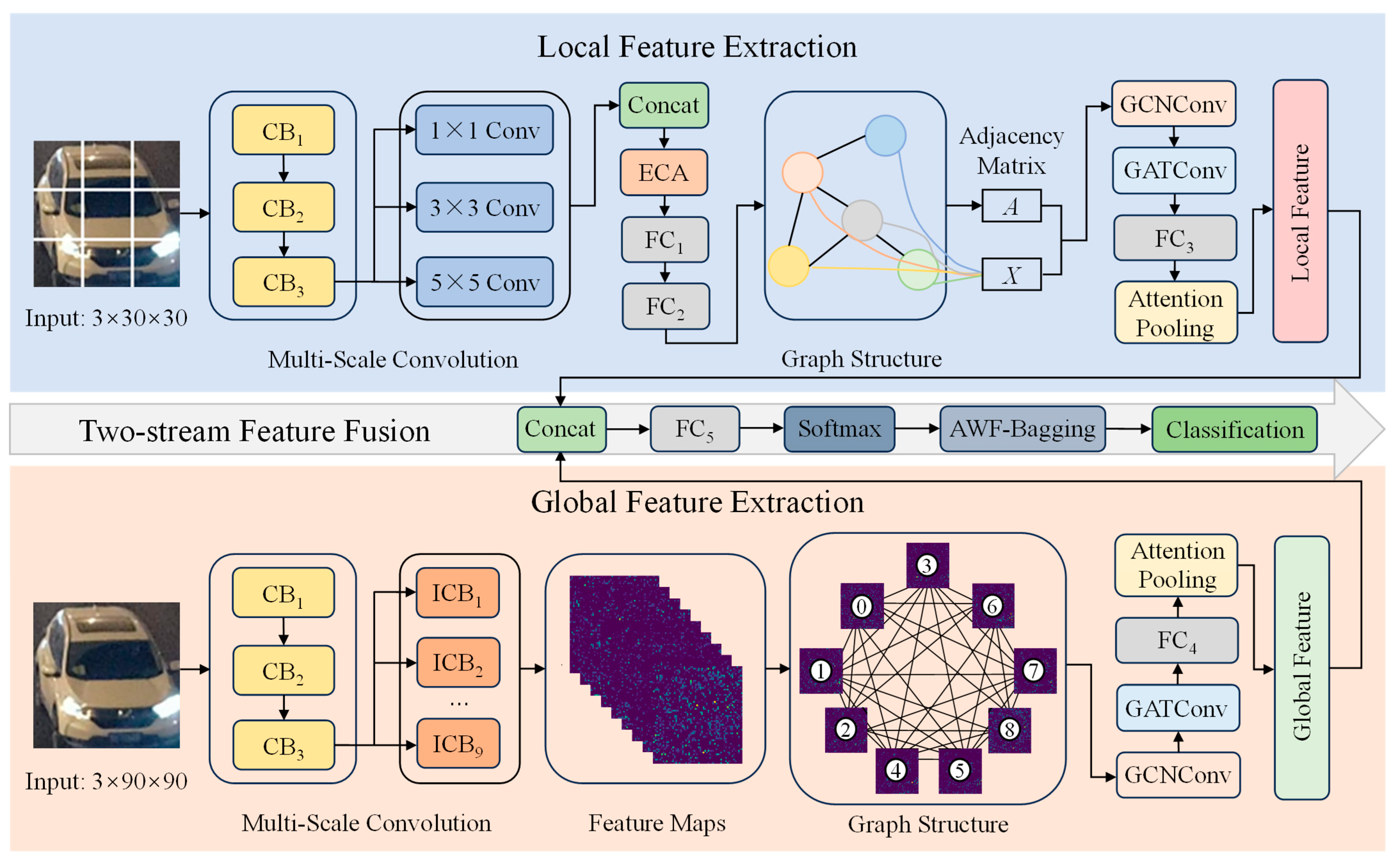
This paper proposes a dual-stream low-light vehicle type recognition model based on GNNs named TFF-Net. The overall model structure is shown in
Figure 1. TFF-Net fuses multi-scale CNN features with hybrid GNN topology-aware graph information to improve recognition performance in complex scenes by collaboratively modeling local and global features.
The local branch (Net1) employs multi-scale convolutional kernels and a channel attention mechanism for fine-grained feature extraction from the segmented image of the nine-box grid. The global branch (Net2) captures contextual information such as contour and color distribution through independent convolutional layers and maps features to fully connected graph nodes. The GNN module combines a GCN and GAT to mine spatial and semantic associations between nodes to generate abstract high-level graph features. The attentional pooling module performs a weighted fusion of global and local features, suppresses the interference of irrelevant information, and finally outputs the classification results through the fully connected layer. For the category imbalance problem, the model introduces dynamic weight adjustment and label smoothing techniques to optimize the loss function. The AWF-Bagging algorithm integrates multiple base classifiers to further improve the robustness and accuracy.
3.1. Two-Stream Feature Extraction
3.1.1. Local Feature Extraction
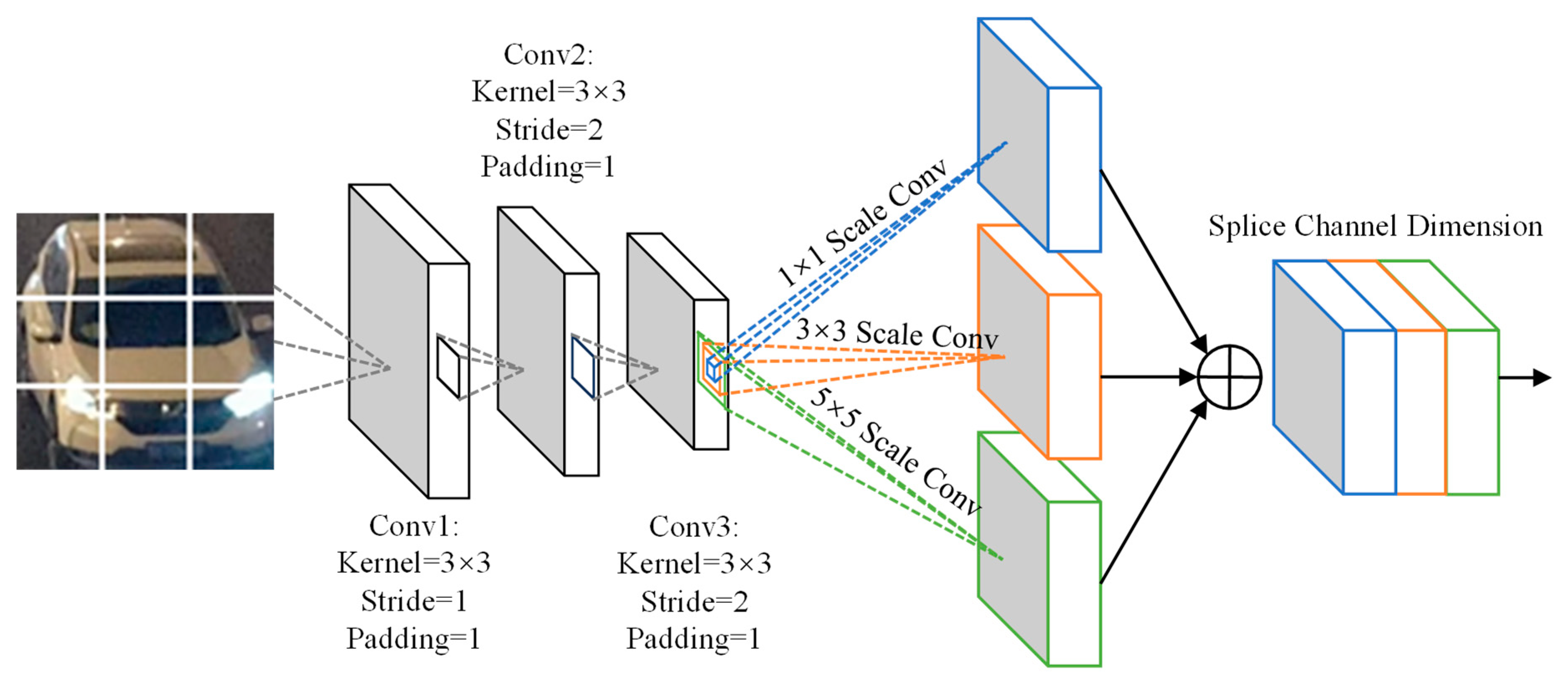
This paper uses a region segmentation method to uniformly divide the input image into 3 × 3 grid regions. This method can force the model to focus on key local structures such as headlights and air intake grilles, thus capturing detailed vehicle local features based on spatial structure. Based on this design, the multi-scale local feature extraction network Net1 uses a three-layer convolutional architecture. As shown in
Figure 2, each convolutional layer is followed by a batch normalization, ReLU activation function, and Dropout layer to prevent overfitting. To enhance its feature discrimination ability in complex backgrounds, the model introduces a multi-scale feature fusion module to handle the output of the third-layer convolution. The module deploys three different scales of convolutional kernels, 1 × 1, 3 × 3, and 5 × 5, in parallel to realize a reduction in channel dimensionality, local texture extraction, and perception of large-scale structures, respectively. Subsequently, the multi-scale output is stitched along the channel dimensions to form a fused feature map.
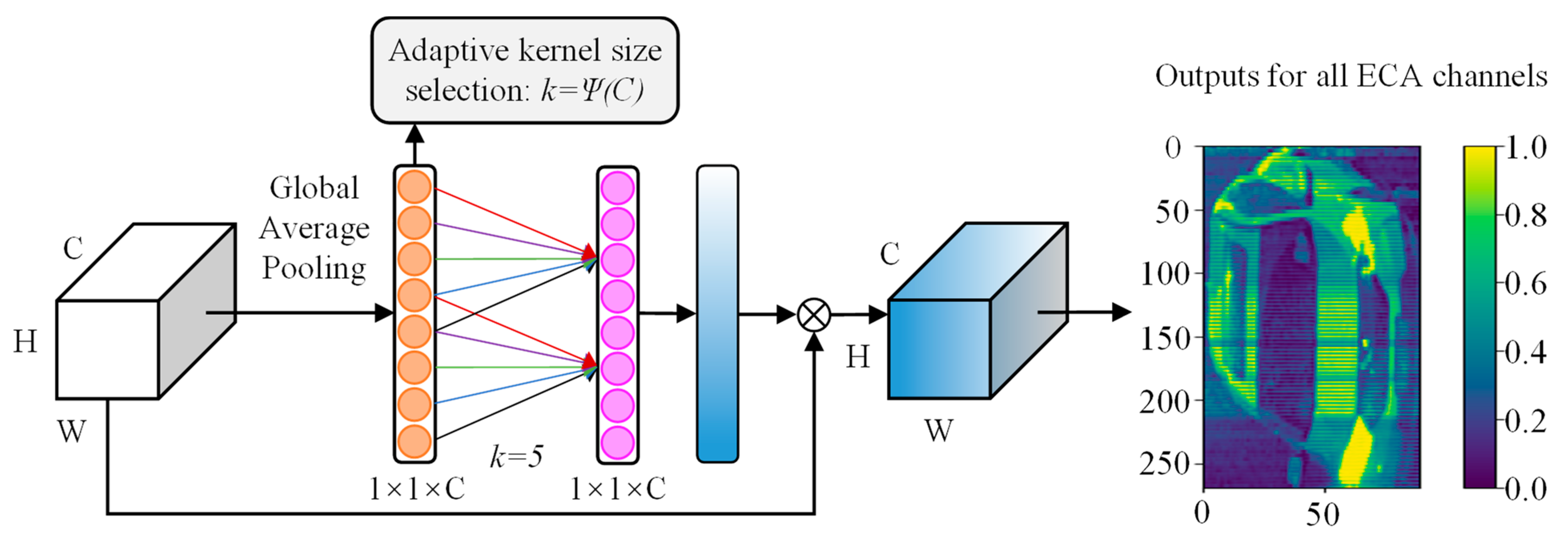
To further enhance the feature representation, the network embeds the ECA channel attention module [
41] after the fusion layer, the structure of which is shown in
Figure 3. The module dynamically calibrates the feature weights of each channel through a lightweight attention mechanism to enhance the feature representation of key channels. After the above processing, the hierarchical feature vectors of the nine grid regions are output. These local features with spatial location information will provide rich node feature representations for the subsequent construction of the graph neural network.
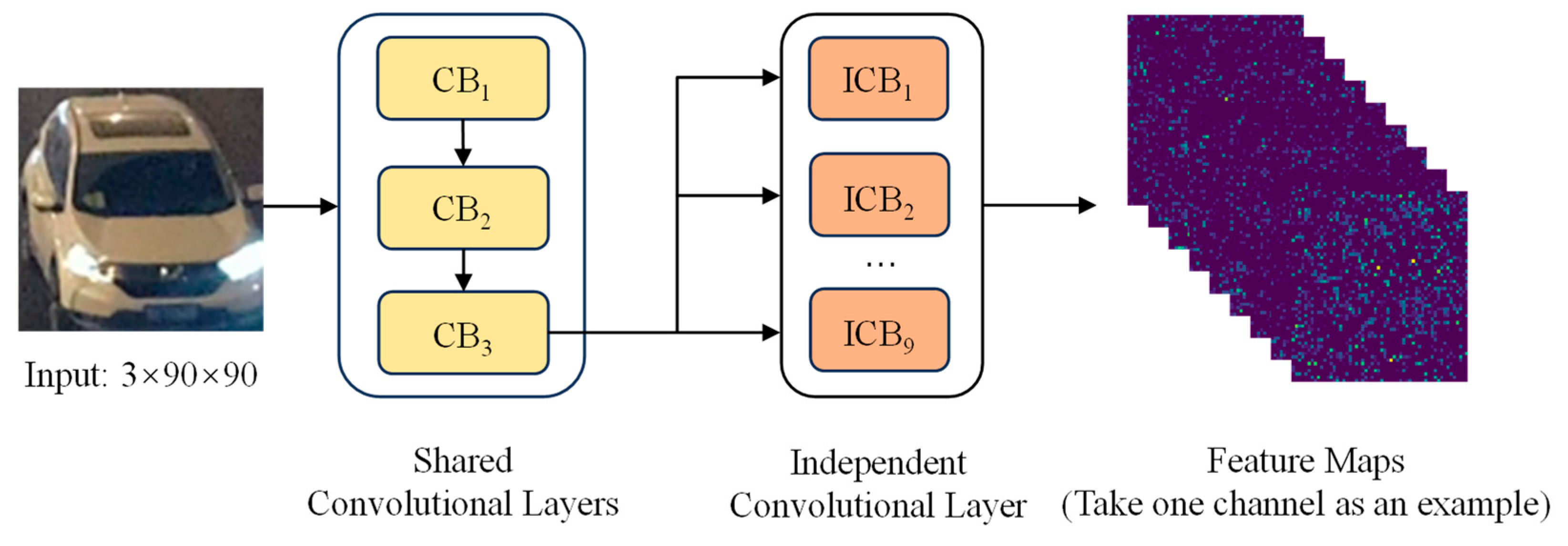
3.1.2. Global Feature Extraction
Due to the influence of complex lighting conditions and a variable vehicle morphology in low-light environments, the traditional single-feature extraction method finds it challenging to satisfy practical needs. Based on the feature map
X3 output from the shared convolutional layer, this paper designs the global feature extraction network Net2, illustrated in
Figure 4. The network utilizes a parallel architecture of nine independent convolutional layers. Each convolutional layer has a unique parameter configuration that enables a multifaceted parsing of the input feature maps from different viewpoints. The independent convolutional layer performs feature extraction on the feature map
through differentiated convolutional kernels to capture diverse global feature information such as the overall vehicle contour, color distribution, and spatial layout.
The output of the
independent convolutional layer is calculated in Equation (1).
where
denotes the convolution operation;
denotes the convolution kernel weight; and
denotes the convolution kernel bias.
Each independent convolutional layer performs a sliding convolution operation on top of the feature map through different convolutional kernels to extract diverse features. During the training process, the convolutional kernel parameters are dynamically adjusted based on backpropagation so that each convolutional layer can adaptively learn feature representations at different scales.
3.2. Feature Fusion Based on Graph Structure Relationship Modeling
3.2.1. Graph Structure Construction
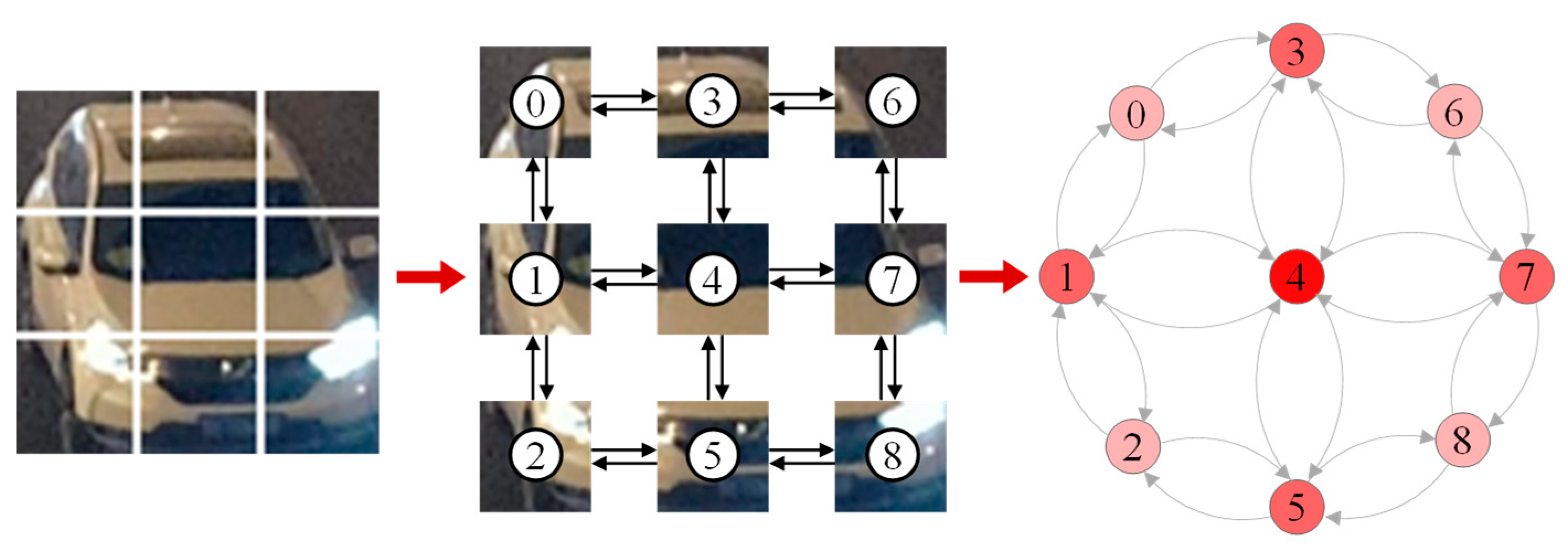
The construction of fully connected graph structures based on spatial adjacencies allows for the modeling and analysis of image topology using graph neural networks. As shown in
Figure 5, the segmented 3 × 3 grid is used as nodes, labeled with ordinal numbers, and edge connections are established based on spatial adjacencies. The color of the ordinal number indicates the size of the degree. The nine grid image features extracted by Net1 are used as spatial association nodes to construct the local graph structure.
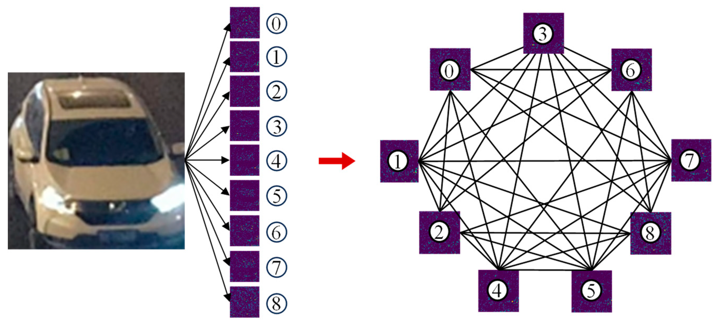
The nine feature maps output from Net2 are converted into node feature vectors by flattening them to form a node feature matrix, and the global graph structure indicated in
Figure 6 is constructed accordingly. To adequately capture the inter-feature correlation, the adjacency matrix adopts the fully connected form so that information can interact between any nodes.
3.2.2. Graph Neural Network Design
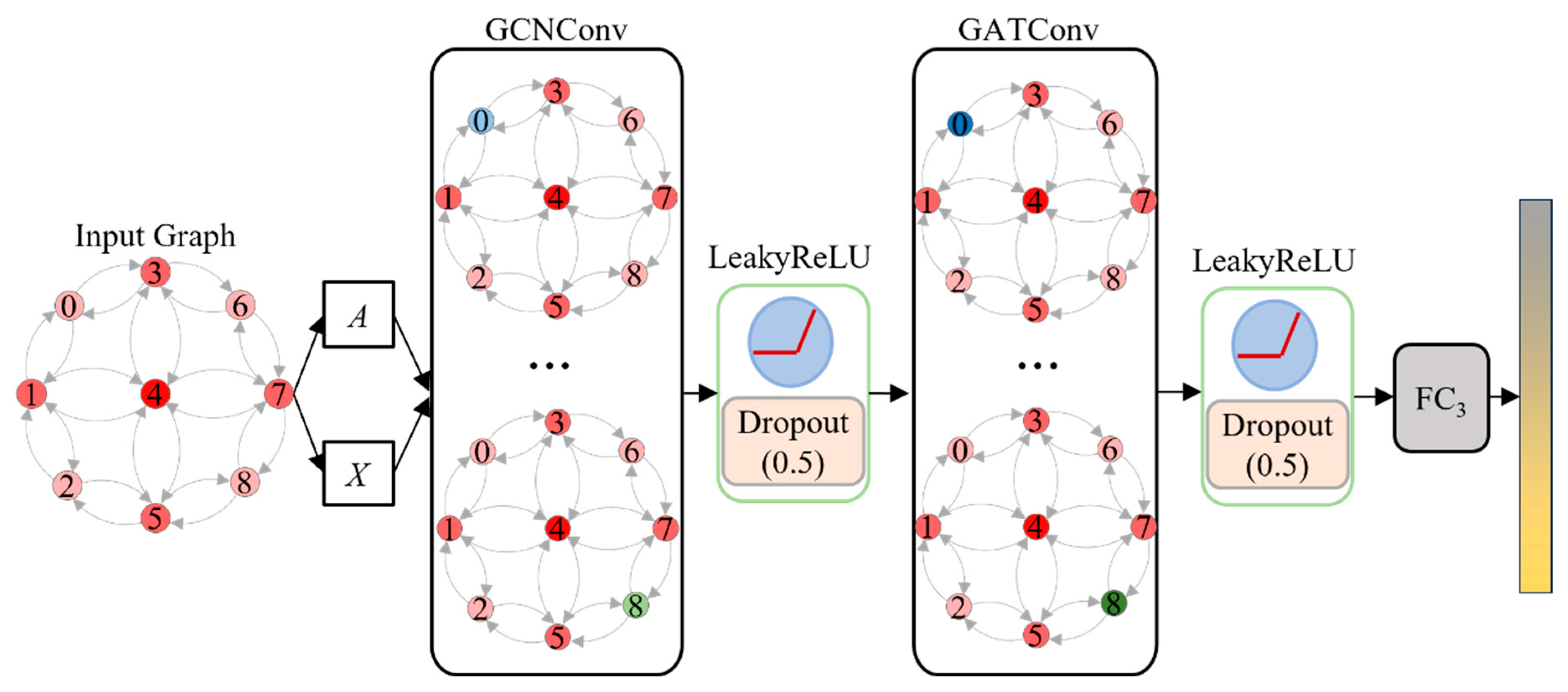
A GCN-GAT hybrid architecture is designed to mine spatial and semantic associations between nodes, dynamically update node features, and entirely mine and integrate advanced features. The GNN structure design is presented in
Figure 7. This architecture uses a low computational complexity GCN layer to aggregate neighbor node feature information for the base propagation and initial fusion of features. The GCN does not consider the heterogeneous feature differences between nodes, so a GAT layer capable of an adaptively weighted fusion of neighboring nodes’ features is introduced. With the hybrid use of GCN and GAT layers, the model can learn more abstract and high-level graph features to improve the accuracy and robustness of vehicle type recognition under low-light conditions.
3.2.3. Feature-Weighted Fusion
Subsequently, the attention pooling module weighted and fused the global and local features to suppress the interference of irrelevant information and obtain a more discriminative feature representation.
Normalization of the attention coefficients
and
by the Softmax function ensures that the weights satisfy
, as follows:
where
and
are learnable parameter matrices.
The global feature vector
and local feature vector
output from the graph neural network are passed through the attention pooling module to obtain features
and
:
where
and
are learnable projection matrices.
Before splicing, global feature (of dimension ) and local feature (of dimension ) are mapped to the uniform dimension through the fully connected layer:
After attentional pooling, the aligned features are directly spliced along the channel dimensions without dimensional conflicts as the final fused features vector
:
The fusion of global and local features after GNN processing can fully utilize the advantages of these two features and reveal their intrinsic connections. Feature fusion provides a more discriminative feature representation for the low-light vehicle type recognition task, thereby improving the model’s effectiveness.
3.3. Loss-Regularization Strategy
A more severe dataset category imbalance exists in vehicle type recognition in low-light environments. The sample size of the minority categories is much smaller than that of the majority category. This can lead to model training guided by the traditional cross-entropy loss function, tending to be biased towards the majority category and affecting the generalizability and usefulness of the overall model. In addition, the model is prone to overfitting when learning real labels represented by the one-hot encoding technique, and this makes the model under-adaptive in the face of unknown data. To solve the above problems, we propose an innovative loss function improvement strategy. This strategy introduces the mechanism of the dynamic adjustment of weights based on the original cross-entropy loss function and combines it with the label smoothing technique.
3.3.1. Dynamic Adjustment of Weighting Mechanism
A dynamic adjustment of the weights mechanism is designed, considering the negative impact of category imbalance on model training. The dynamic weights
are calculated as follows:
where
denotes the number of samples in the
category in the current round
.
During the training process, the categories with small samples correspond to larger weights. The model is forced to pay more attention to these few categories of samples to avoid neglecting a few categories due to category imbalance. Based on the above dynamic weights, the improved loss function is shown in Equation (8).
where
is the number of categories,
is the one-hot encoding of the true label
of the sample, and
is the probability value predicted by the model.
3.3.2. Label Smoothing Technique
In practice, data is often noisy and from anomalous samples. The overconfidence of the model in the training data leads to a degradation in its performance on the test set, hence the introduction of label smoothing techniques [
42]. The original true labeling
is adjusted to smooth the distribution
:
where
denotes the smoothing parameter, which usually takes a value between 0.1 and 0.2, with the actual value of 0.1.
Via smoothing, the true labels are no longer certain but spread to other categories to some extent. This makes the model less dependent on single-category determinism and more robust in its learning process. After incorporating label smoothing in the loss function, a new loss function,
, is obtained.
The final improved loss function
in Equation (11) is obtained by combining the dynamic weighting mechanism with the label smoothing technique.
After the fused features are fed into the fully connected layer, the model training is optimized by combining the improved cross-entropy loss function to solve the category imbalance problem. This function effectively solves the limitation of traditional cross-entropy loss and provides a more reliable basis for model training and practical applications under complex data distributions.
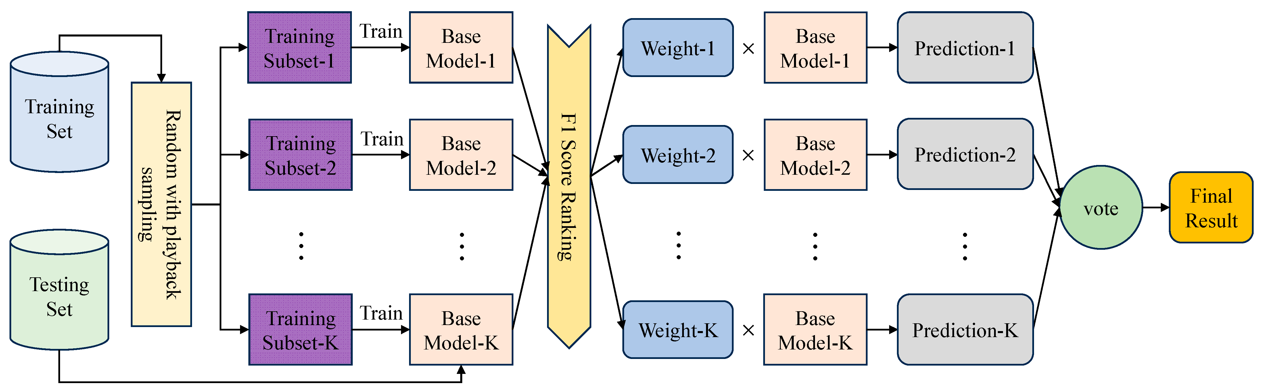
3.4. AWF-Bagging Algorithm Integration
To strengthen the model’s ability to adapt to data heterogeneity and noise, the Adaptive Weighted Fusion-Bagging (AWF-Bagging) algorithm is proposed for multi-classification tasks. Unlike traditional Bagging, where equal weights are averaged or voted, AWF-Bagging assigns differentiated weights to each classifier based on the performance of the base classifiers (F1 scores). Its structure is illustrated in
Figure 8.
Obtain the F1 scores of the base classifiers on the test set, rank the F1 scores, and assign the corresponding weights. The weight assignment follows the normalization constraint (sum to 1), which is calculated in Equation (12).
where
means the weight of the
base classifier,
means the F1 score of the
base classifier, and
means the total number of base classifiers.
High-performance base classifiers are given a higher weight in the integration decision, and low-performance classifiers are suppressed. This mechanism allows the model to automatically adapt to data distribution heterogeneity and differences in the performance of base classifiers rather than relying on fixed rules. Traditional Bagging’s equal-weighted averaging does not allow for this optimization.
For the integration, the predictions of the base classifiers are multiplied by their weights and then accumulated. The final output of the Bagging Heterogeneous Integration Model is obtained as shown in Equation (13).
where
is the integrated model’s final output, which indicates each category’s probability distribution in the multiclassification task, and
indicates the prediction result of the
base classifier on the input
.
A probability threshold,
, is set to determine whether the input
belongs to a particular category, The specific determination of the category label
is shown in Equation (14).
where
denotes the prediction probability of the integrated model for the first category.
AWF-Bagging is based on base classifiers and uses an adaptive weighted fusion strategy to integrate the prediction results of each base classifier. The constructed feature fusion model is used as a base classifier. independent base classifiers are constructed. The base classifiers are trained using different training subsets. The base classifiers are trained independently and optimized with hyperparameters to finally generate their respective classifiers , where . In the testing phase, weights are assigned based on the F1 scores of the base classifiers on the test set. The predictions of the base classifiers are weighted and fused to obtain the final output of the integrated model. By setting a probability threshold of , the category to which the input belongs is determined.
The application of the AWF-Bagging algorithm to the model can effectively utilize the performance difference of the base classifiers to improve the classification accuracy and the model’s robustness.
4. Dataset
Vehicle datasets play an essential role in autonomous driving and intelligent transportation. They can provide rich data support for tasks such as vehicle detection, tracking, and classification.
Table 1 compares four common publicly available vehicle datasets.
The existing datasets have significant shortcomings regarding surveillance viewpoints and the coverage of extreme low-light environments, which hardly reflect complex traffic realities. This study constructs a novel low-light surveillance viewpoint vehicle dataset, VDD-Light.
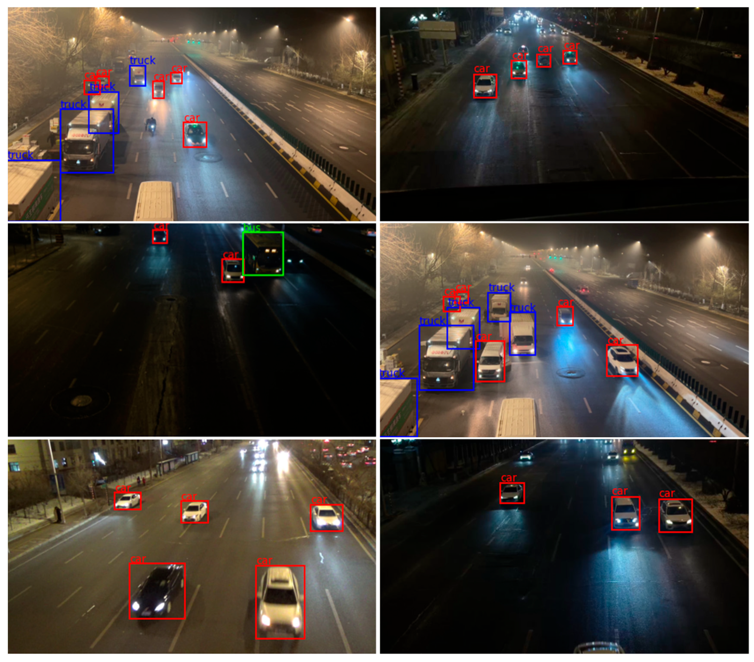
Figure 9 presents the nine images in the VDD-Light dataset and the corresponding labeling results.
A Sony HDR-CX680 camera (Shanghai Suoguang Video Co., Ltd., Shanghai, China.) is used to obtain 26 low-light traffic flow videos by shooting from overhead at the flyover locations of Hexing Road and Xuefu Road sections in Harbin City. The video is disassembled at 30 frames per second, and 5468 standardized images of 3840 × 2160 pixels are filtered. Based on the actual application requirements, we have established a labeling system that includes three types of targets: car, bus, and truck. Image annotation is performed in VOC format and convert to YOLO algorithm-adapted format, with the annotation information covering target categories and normalized bounding box coordinates. The vehicle detection dataset is divided into 3827 images for the training set, 1094 images for the validation set, and 547 images for the test set, according to the ratio of 7:2:1. The UA-DETRAC public dataset involving nighttime surveillance camera shots is chosen as the supplementary test data to validate the model’s performance in the vehicle type recognition task. The images in the UA-DETRAC dataset that are eligible for low illumination are filtered to construct a high-quality test dataset. The VDD-Light dataset effectively supports the model’s performance evaluation in real traffic surveillance scenarios and low-light environments.
The labeled vehicles are intercepted from the image to construct the low-light vehicle classification dataset VC-Data. Samples of the car class are downsampled, and data enhancement, including affine transformation, level flipping, Gaussian blurring, contrast adjustment, and brightness adjustment, is performed on the bus and truck class samples. The VC-Data dataset is divided into a training set and a test set in a ratio of 8:2, which serves as the basis for model training and validation.
Table 2 sets out the vehicle classes and the corresponding number of images for the VC-Data dataset.
The self-built vehicle classification dataset VC-Data lays the foundation for evaluating the proposed low-light vehicle type recognition model’s performance. The self-built vehicle detection dataset VDD-Light supports the testing of the model’s performance.
5. Experiment
5.1. Implementation Details
Table 3 lists detailed experimental environments for this experiment. To fully utilize the computational resources and achieve the optimal training effect, the parameters of the TFF-Net model are set as follows: the Adam optimizer is used, the batch size is 1, the epoch is 100, the learning rate is set to 0.001 and reduced to 0.9 times the original one after 10 iterations, and the L2 regularization coefficient is 0.0001. The parameters for the YOLO are set as follows: using the SGD optimizer with a batch size of 64, an epoch of 100, and an initial learning rate set to 0.01. For the other comparison methods, the corresponding parameter adjustment and optimization are carried out according to their respective characteristics to ensure the best performance in the experiment.
5.2. Experimental Evaluation Metrics
Six metrics evaluate the model’s multi-classification and target detection task performance. Accuracy measures the model’s overall predictive accuracy. Precision (P) values the proportion of True Positive results in a prediction. Recall (Recall, R) quantifies the coverage of actual positive results. Mean Average Precision (mAP) assesses the robustness of the multi-class detection. The mAPs used include an average precision mAP50 at 50% of the intersection and union ratio (IoU) threshold and an average precision mAP50-95 in the range of 50% to 95% of the IoU threshold. The number of parameters (Params) indicates the spatial complexity of the model.
The calculation method of each evaluation index is shown in Equations (15)–(20).
where
is the True Positive class and represents the number of classes that the model correctly predicts as positive;
is the False Negative class and indicates the number of positive classes that the model incorrectly predicts as negative;
is the False Positive class, which shows the number of negative classes that the model incorrectly predicts as positive;
is the True Negative class and indicates the number of classes that the model correctly predicts as negative.
denotes the area enclosed by the PR curve and the axes;
means the number of tested sample categories.
5.3. Results and Discussion
5.3.1. Module Validity Experiments
Experiments are designed on the VC-Data dataset to validate the effectiveness of each module in the proposed model’s feature extraction and mining phase. The M1, M2, M3, M4, and M5 models are specified by sequentially removing the multi-scale convolutional kernel, the channel attention mechanism (ECA Block), the GCN convolutional layer (i.e., entirely using GAT layers), and the GAT convolutional layer (i.e., entirely using GCN layers). The accuracy is used as a criterion to verify the validity of the module sequentially, and the results are presented in
Table 4.
Based on the experimental results, each module in the proposed model’s feature extraction and mining phase plays a vital role in the performance’s improvement. The multi-scale convolutional kernel improves the accuracy by 2.00% by capturing features at different scales, which proves the significance of an enhanced feature richness. Model accuracy decreases by 2.97% after the ECA channel attention mechanism is removed, highlighting its ability to screen key feature channels. Both GCN and GAT layers are used in conjunction with each other to improve the accuracy by 1.50% and 1.00%, respectively, compared to a single structure, which reflects the effectiveness of mining graph structure features with a mixture of GCNs and GATs. These modules complement each other in feature extraction, feature screening, information dissemination, and relationship mining, resulting in a 93.25% accuracy in recognizing vehicle types in low-illumination environments.
5.3.2. Experiments on Overall Model Performance
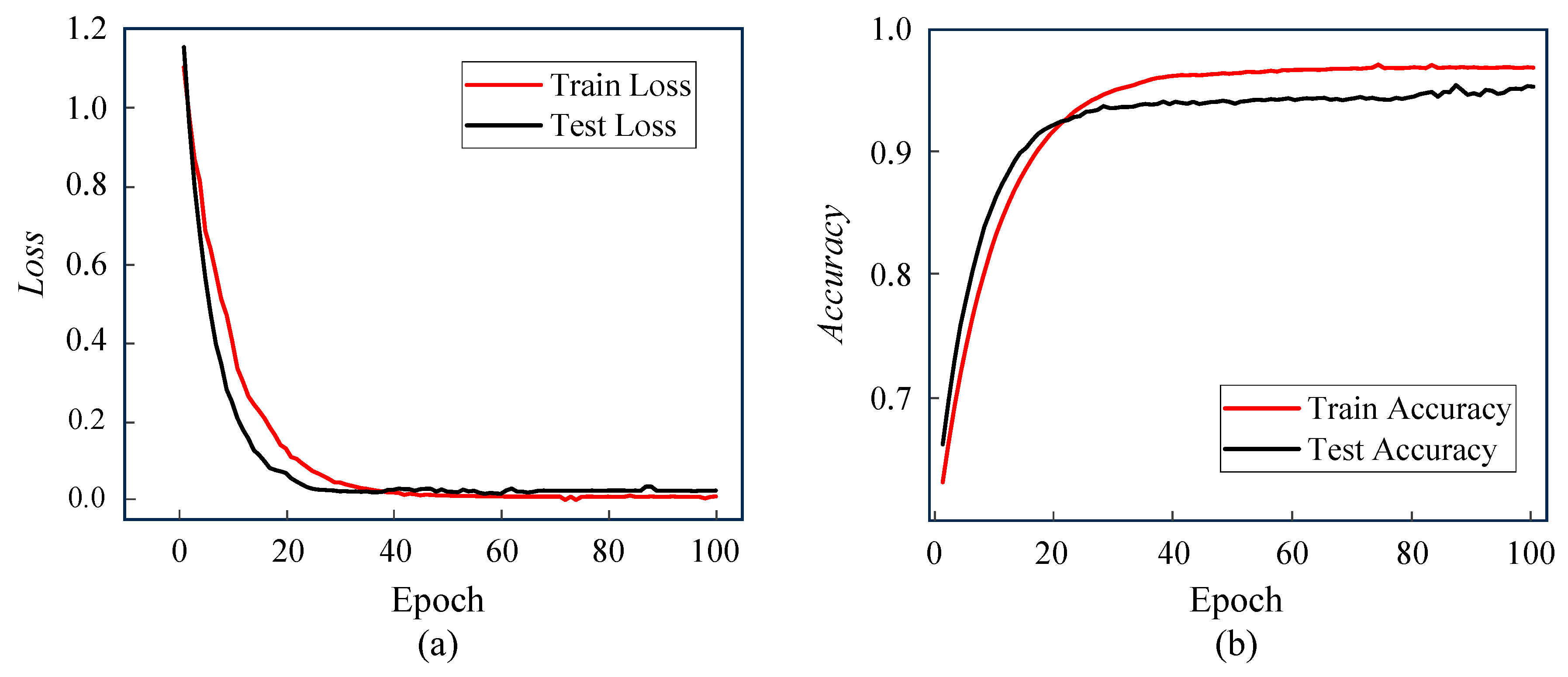
The overall vehicle type recognition model’s performance in low-illumination environments is trained and tested. The obtained loss and accuracy curves are presented in
Figure 10.
From
Figure 10a’s loss curves, Train Loss and Test Loss plummet and stabilize at the beginning of training (first 40 rounds). This shows that the model converges efficiently and without overfitting.
Figure 10b displays that the training accuracy rises from 60% to nearly 90%, and the test accuracy increases simultaneously. The growth rate slows down and eventually stabilizes around 95% after 20 rounds, which reflects the model’s good generalizability. Together, both types of curves validate the data quality and model design.
After the experimental training and testing, the specific values of the evaluation indicators corresponding to each category (car, bus, truck) are obtained and summarized in
Table 5.
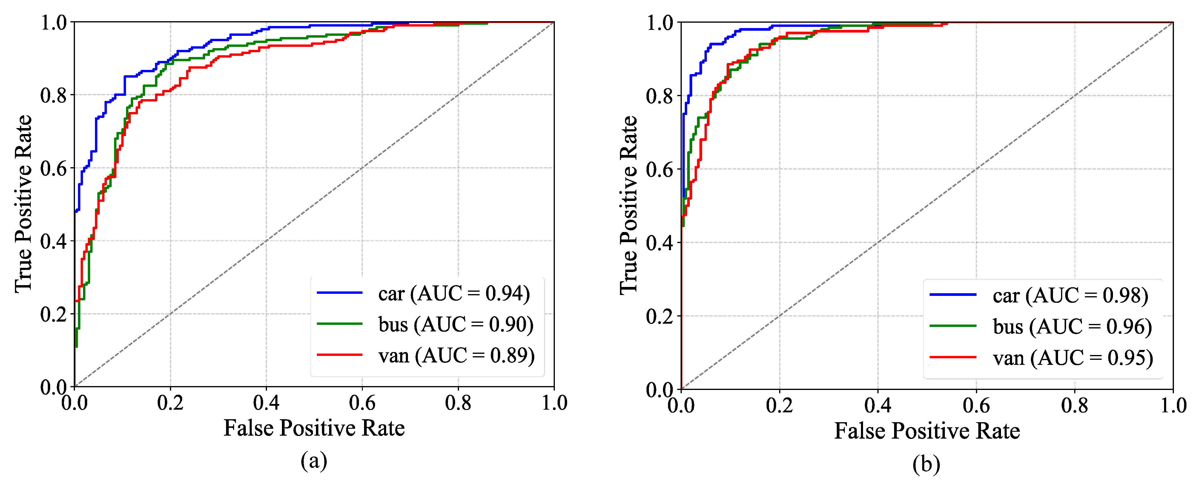
The ROC curves for the M5 model and the TFF-Net model are illustrated in
Figure 11. Intuitively, from the curve morphology, TFF-Net makes a significant improvement in the classification performance of each category. The curves are more closely aligned towards the upper left corner, which means TFF-Net is able to recognize the positive case samples more accurately and reduce the occurrence of misclassification situations.
The low-light vehicle recognition model TFF-Net proposed in this paper shows excellent performance in the test set, with an overall accuracy of 0.9573. TFF-Net has optimal precision (0.9842), recall (0.9564), and F1 values (0.9701) in the car category. The F1 values for the bus and truck categories are 0.9467 and 0.9424, respectively, significantly narrowing the inter-category performance differences compared to the M5 model. It is shown by the multi-dimensional evaluation that the effectiveness and robustness of the proposed model for vehicle type recognition in low-light environments are fully verified.
5.3.3. Ablation Experiments
Ablation experiments are performed on the VC-Data dataset to validate the effectiveness of each module in the overall TFF-Net model. The specific operation is to add feature fusion, AWF-Bagging, and the improved loss function sequentially based on the M5 model to constitute the M6, M7, M8, and TFF-Net models. Each module is verified in turn for its role in the network in terms of accuracy, and the results of the ablation experiments are shown in
Table 6.
The experimental results show that the progressive optimization strategy in this paper significantly enhances the performance of the low-light vehicle recognition model. With the introduction of the multi-scale feature fusion module, the accuracy is improved by 1.08%, and the synergistic modeling of local features and global representations enhances the feature expression capability. The AWF-Bagging algorithm is further adopted to improve the accuracy by 0.84% to 95.17%. This algorithm effectively coordinates the performance differences among base classifiers through a dynamic weight allocation, strengthening the model’s ability to adapt to data heterogeneity. After the improved loss function is employed, the model accuracy reaches a peak of 95.73%, which suppresses overfitting while improving the robustness of classification in uncertain environments. The proposed model breaks through the limitations of traditional methods from the three dimensions of feature characterization, model generalization, and decision boundaries, respectively, and provides a systematic solution for vehicle recognition under complex lighting conditions.
5.3.4. Comparison Experiments
Comparison experiments are designed to verify the effectiveness of the proposed vehicle type recognition model for low-light environments. The model’s performance is quantitatively compared to benchmark methods such as ResNet50, AlexNet, SVM-HOG, and Faster R-CNN.
Table 7 shows the results of the model-specific comparisons.
The experimental results show that TFF-Net is significantly superior to the comparison method in all evaluation indexes. In terms of macro evaluation indicators, Macro-Precision, Macro-Recall, and Macro-F1 reached 0.9490, 0.9576, and 0.9531, respectively, which are all significantly improved. The results confirm the effectiveness of TFF-Net in dealing with the category imbalance problem and the model’s reliability in vehicle type recognition in low-light environments.
5.3.5. Significance Analysis Experiments
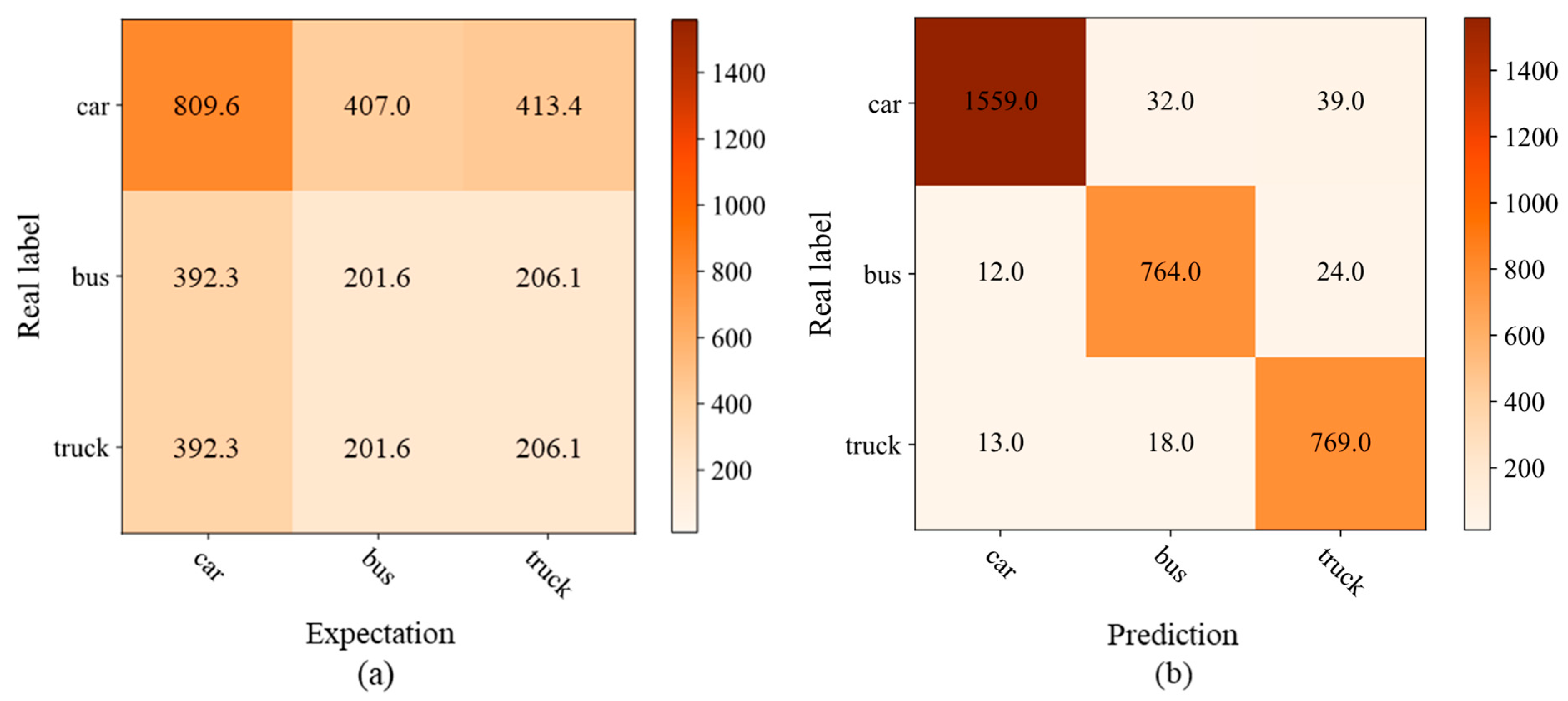
A confusion matrix is a tool used to represent the classification results of the model on the test set. It can help to evaluate the performance of the model and analyze the type of errors. After experimental training and testing, the confusion matrix corresponding to each category (car, bus, truck) is obtained, as illustrated in
Figure 12b. The expected frequencies under the assumption of random guessing are calculated, as shown in
Figure 12a.
Calculating the chi-square statistic () based on the observed values (values in the confusion matrix) and the expected values yields 5586.7 for a three-class classification problem with a degree of freedom of four, which ultimately computes a p-value much less than 0.05. Since the p-value is much less than 0.05, we reject the original hypothesis and conclude that there is a significant difference between the model’s classification results and random guessing. This indicates that the proposed model’s classification performance is significantly better than random guessing.
5.3.6. Target Detection Performance Test Experiments
One-stage deep learning methods include the YOLO series [
47,
48], of which YOLOv11n [
49] is the latest lightweight model. The original convolutional classification head of YOLOv11n adopts the regular mesh feature extraction mechanism, which suffers from an insufficient capability to model the topology among vehicle parts and the poor robustness of the features in low-illumination and occlusion scenes. To this end, this paper presents the target detection algorithm YOLOv11-TFF by introducing the proposed TFF-Net instead of the original classification head. YOLOv11-TFF follows the improved cross-entropy loss function. The algorithm combines the efficient localization capability of YOLOv11n with the graph neural network feature modeling advantage of TFF-Net to achieve the accurate positioning and reliable classification of vehicles in low-illumination environments.
The improved YOLOv11n algorithm is compared with the current mainstream target detection algorithms to verify the reliability and good detection performance of YOLOv11-TFF.
Table 8 shows the experimental results of the comparison of Precision, Recall, mAP50, and the number of parameters (Params) for each algorithm on the test set.
Table 8 illustrates that YOLOv11-TFF performs outstandingly compared with other models, with a Precision of 0.958, Recall of 0.969, mAP50 as high as 0.987, and mAP50-95 of 0.914. This indicates that the model has less misclassifications and an accurate recognition and can effectively detect real vehicle targets. The proposed model has a high detection accuracy under different IoU thresholds, demonstrating adaptability and robustness. The number of parameters of YOLOv11-TFF is 4.26 × 10⁶, which ensures high accuracy with reasonable complexity and achieves a favorable balance between accuracy and resource requirements.
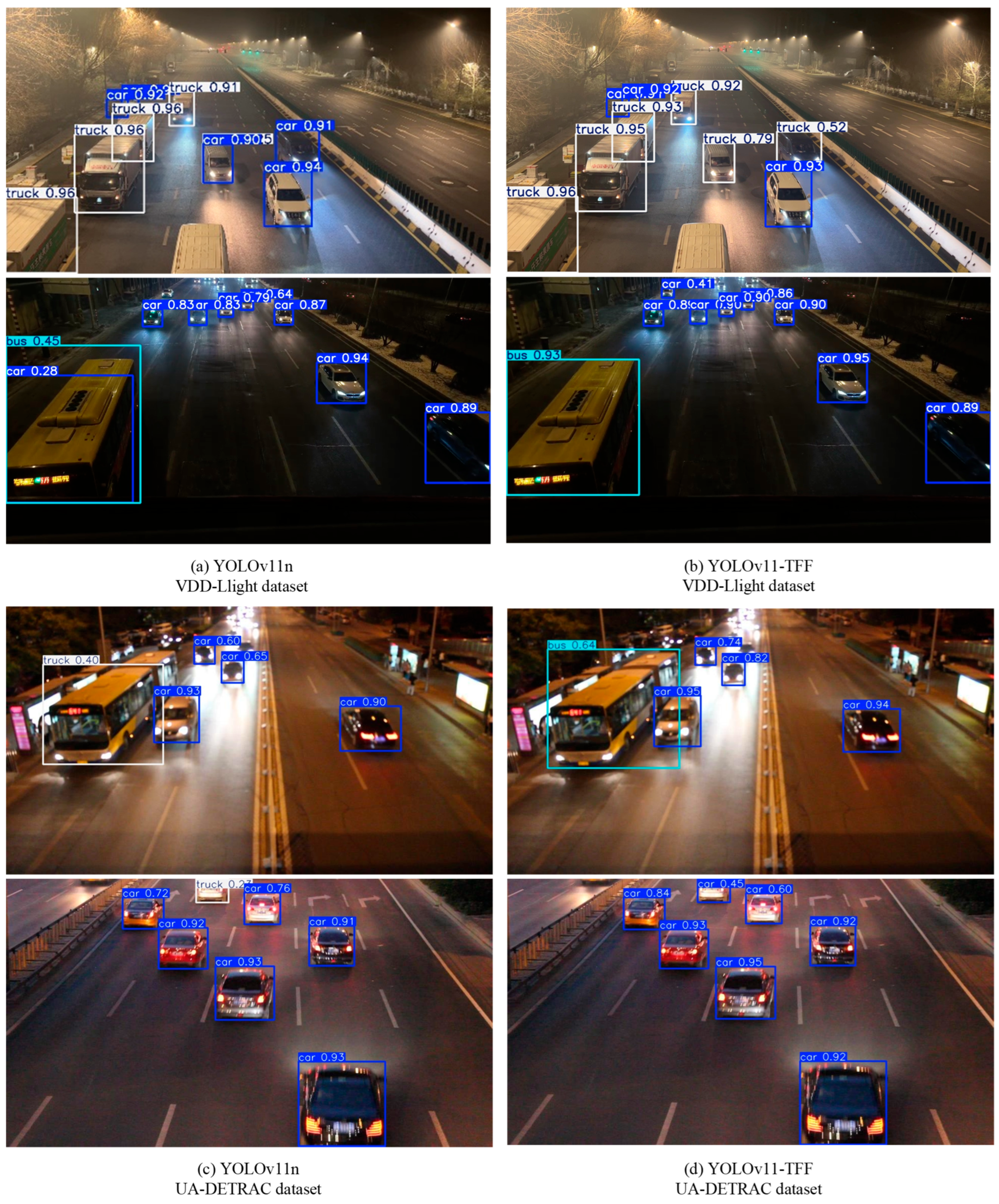
The performance of the YOLOv11-TFF algorithm is validated using the self-built VDD-Light low-light environment vehicle detection dataset and the UA-DETRAC public dataset.
Figure 13 sets forth a comparison of the target detection results for YOLOv11n and YOLOv11-TFF.
As shown in the results of the visualization evaluation, YOLOv11-TFF is able to recognize models stably in a variety of low-light real-world application scenarios. The proposed method can correctly identify the vehicle type even in poorly lit areas or when the target vehicle is far away. It shows that YOLOv11-TFF is highly adaptable and stable in low-light environments, which lays a solid foundation for the algorithm’s large-scale promotion in practical applications.
6. Conclusions
This paper designs and optimizes a model using graph neural networks to address the shortcomings of existing vehicle type recognition in low-light environments. We build local–global two-stream feature extraction networks containing multilevel convolution and map the output features to nodes constructed as graph structures. A hybrid GNN architecture is designed to enhance feature expression. The output features of the GNN layer are fused to achieve vehicle type recognition and classification after the attention pooling module. Enhanced model stability and generalization are achieved using the improved adaptive weighting AWF-Bagging algorithm. Meanwhile, the dynamic adjustment weight mechanism and label smoothing technique are introduced to optimize the loss function and solve the category imbalance and overfitting problems. For the recognition and classification tasks, the TFF-Net model achieves an overall accuracy of 95.4% on the test set. After integration with the target detection algorithm, the YOLOv11-TFF algorithm achieves a mAP of 91.4%, with a model parameter count of 4.26 M. The proposed model can realize high-precision vehicle recognition and is expected to be deployed in edge computing devices, which verifies the practical value of the model in real traffic monitoring scenarios based on camera sensors. This paper also has some limitations, and the subsequent research will focus on making the model lightweight and applications in complex weather scenarios such as rain, snow, and fog.
Author Contributions
Conceptualization, Resources, Writing—review and editing, Funding acquisition, H.X.; Conceptualization, Methodology, Writing—original draft, W.T.; Software, Validation, Writing—original draft, Data curation, Y.L.; Writing—review and editing, Supervision, Y.T. All authors have read and agreed to the published version of the manuscript.
Funding
This work is supported by the Natural Science Foundation Project of Heilongjiang Province (Grant No. PL2024E012).
Institutional Review Board Statement
Not applicable.
Informed Consent Statement
Not applicable.
Data Availability Statement
The original contributions presented in this study are included in the article. Further inquiries can be directed to the corresponding author.
Conflicts of Interest
The authors declare no conflicts of interest.
References
- Yang, S.; Zhou, L.; Zhang, Z.; Sun, S.; Guo, L. Examining the correlation of household electric vehicle ownership: Insights for emerging mobility and planning. J. Transp. Geogr. 2024, 118, 103937. [Google Scholar] [CrossRef]
- Gan, L.; Chu, W.; Li, G.; Tang, X.; Li, K. Large models for intelligent transportation systems and autonomous vehicles: A survey. Adv. Eng. Inf. 2024, 62, 102786. [Google Scholar] [CrossRef]
- Bekelcho, T.; Birgoda, G.T.; Leul, H.; Maile, M.; Alemayehu, M.; Olani, A.B. Near miss road traffic accidents and associated factors among truck drivers in Gamo zone, southern Ethiopia by using a contributory factors interaction model. Front. Public Health 2024, 12, 1386521. [Google Scholar] [CrossRef]
- Zhou, B.; Feng, Z.; Liu, J.; Huang, Z.; Gao, Y. A method to enhance drivers’ hazard perception at night based on “knowledge-attitude-practice” theory. Accid. Anal. Prev. 2024, 200, 107565. [Google Scholar] [CrossRef] [PubMed]
- Tan, S.H.; Chuah, J.H.; Chow, C.O.; Kanesan, J.; Leong, H.Y. Artificial intelligent systems for vehicle classification: A survey. Eng. Appl. Artif. Intell. 2024, 129, 107497. [Google Scholar] [CrossRef]
- Mei, M.; Zhou, Z.; Liu, W.; Ye, Z. GOI-YOLOv8 Grouping Offset and Isolated GiraffeDet Low-Light Target Detection. Sensors 2024, 24, 5787. [Google Scholar] [CrossRef]
- Wang, K.; Guo, J.; Chen, K.; Lu, J. An in-depth examination of SLAM methods: Challenges, advancements, and applications in complex scenes for autonomous driving. IEEE Trans. Intell. Transp. Syst. 2025, 1–22. [Google Scholar] [CrossRef]
- Archana, R.; Jeevaraj, P.E. Deep learning models for digital image processing: A review. Artif. Intell. Rev. 2024, 57, 11. [Google Scholar] [CrossRef]
- Zhao, X.; Wang, L.; Zhang, Y.; Han, X.; Deveci, M.; Parmar, M. A review of convolutional neural networks in computer vision. Artif. Intell. Rev. 2024, 57, 99. [Google Scholar] [CrossRef]
- Chen, C.; Wu, Y.; Dai, Q.; Zhou, H.-Y.; Xu, M.; Yang, S. A survey on graph neural networks and graph transformers in computer vision: A task-oriented perspective. IEEE Trans. Pattern Anal. Mach. Intell. 2024, 46, 10297–10318. [Google Scholar] [CrossRef]
- Kipf, T.N.; Welling, M. Semi-supervised classification with graph convolutional networks. arXiv 2017, arXiv:1609.02907. [Google Scholar]
- Veličković, P.; Cucurull, G.; Casanova, A.; Romero, A.; Lio, P.; Bengio, Y. Graph attention networks. arXiv 2017, arXiv:1710.10903. [Google Scholar]
- Yan, S.; Xiong, Y.; Lin, D. Spatial temporal graph convolutional networks for skeleton-based action recognition. In Proceedings of the Thirty-Second AAAI Conference on Artificial Intelligence (AAAI-18), New Orleans, LA, USA, 2–7 February 2018; pp. 7444–7452. [Google Scholar] [CrossRef]
- Fu, H.; Ma, H.; Liu, Y.; Lu, D. A vehicle classification system based on hierarchical multi-SVMs in crowded traffic scenes. Neurocomputing 2016, 211, 182–190. [Google Scholar] [CrossRef]
- Gao, Y.; Lee, J.H. Car manufacturer and model recognition based on scale invariant feature transform. Int. J. Comput. Vis. Robot. 2018, 8, 32–41. [Google Scholar] [CrossRef]
- Chaudhary, S.; Sharma, A.; Khichar, S.; Meng, Y.; Malhotra, J. Enhancing autonomous vehicle navigation using SVM-based multi-target detection with photonic radar in complex traffic scenarios. Sci. Rep. 2024, 14, 17339. [Google Scholar] [CrossRef]
- Chandrasekar, S.K.; Geetha, P. A new formation of supervised dimensionality reduction method for moving vehicle classification. Neural Comput. Appl. 2021, 33, 7839–7850. [Google Scholar] [CrossRef]
- Zhang, L.; Xu, W.; Shen, C.; Huang, Y. Vision-Based On-Road Nighttime Vehicle Detection and Tracking Using Improved HOG Features. Sensors 2024, 24, 1590. [Google Scholar] [CrossRef] [PubMed]
- Alghamdi, A.S.; Saeed, A.; Kamran, M.; Mursi, K.T.; Almukadi, W.S. Vehicle Classification Using Deep Feature Fusion and Genetic Algorithms. Electronics 2023, 12, 280. [Google Scholar] [CrossRef]
- Pemila, M.; Pongiannan, R.K.; Narayanamoorthi, R.; AboRas, K.M.; Youssef, A. Application of an ensemble CatBoost model over complex dataset for vehicle classification. PLoS ONE 2024, 19, e0304619. [Google Scholar] [CrossRef]
- Gholamalinejad, H.; Khosravi, H. Vehicle classification using a real-time convolutional structure based on DWT pooling layer and SE blocks. Expert Syst. Appl. 2021, 183, 115420. [Google Scholar] [CrossRef]
- Dong, X.; Shi, P.; Tang, Y.; Yang, L.; Yang, A.; Liang, T. Vehicle Classification Algorithm Based on Improved Vision Transformer. World Electr. Veh. J. 2024, 15, 344. [Google Scholar] [CrossRef]
- Li, Y.; Wang, J.; Huang, J.; Li, Y. Research on Deep Learning Automatic Vehicle Recognition Algorithm Based on RES-YOLO Model. Sensors 2022, 22, 3783. [Google Scholar] [CrossRef] [PubMed]
- Farid, A.; Hussain, F.; Khan, K.; Shahzad, M.; Khan, U.; Mahmood, Z. A Fast and Accurate Real-Time Vehicle Detection Method Using Deep Learning for Unconstrained Environments. Appl. Sci. 2023, 13, 3059. [Google Scholar] [CrossRef]
- Khemani, B.; Patil, S.; Kotecha, K.; Tanwar, S. A review of graph neural networks: Concepts, architectures, techniques, challenges, datasets, applications, and future directions. J. Big Data 2024, 11, 18. [Google Scholar] [CrossRef]
- Gori, M.; Monfardini, G.; Scarselli, F. A new model for learning in graph domains. In Proceedings of the 2005 IEEE International Joint Conference on Neural Networks, Montreal, QC, Canada, 31 July–4 August 2005; pp. 729–734. [Google Scholar]
- Raj, M.S.; George, S.N.; Raja, K. Leveraging spatio-temporal features using graph neural networks for human activity recognition. Pattern Recognit. 2024, 150, 110301. [Google Scholar] [CrossRef]
- Wang, K.; Ding, Y.; Han, S.C. Graph neural networks for text classification: A survey. Artif. Intell. Rev. 2024, 57, 190. [Google Scholar] [CrossRef]
- Rahmani, S.; Baghbani, A.; Bouguila, N.; Patterson, Z. Graph neural networks for intelligent transportation systems: A survey. IEEE Trans. Intell. Transp. Syst. 2023, 24, 8846–8885. [Google Scholar] [CrossRef]
- Ganesan, P.; Jagatheesaperumal, S.K.; Hassan, M.M.; Pupo, F.; Fortino, G. Few-shot image classification using graph neural network with fine-grained feature descriptors. Neurocomputing 2024, 610, 128448. [Google Scholar] [CrossRef]
- Ding, Y.; Zhang, Z.; Zhao, X.; Cai, W.; He, F.; Cai, Y.; Cai, W.W. Deep hybrid: Multi-graph neural network collaboration for hyperspectral image classification. Def. Technol. 2023, 23, 164–176. [Google Scholar] [CrossRef]
- Hanachi, R.; Sellami, A.; Farah, I.R.; Mura, M.D. Multi-view graph representation learning for hyperspectral image classification with spectral–spatial graph neural networks. Neural Comput. Appl. 2024, 36, 3737–3759. [Google Scholar] [CrossRef]
- Hu, H.; Ding, Y.; He, F.; Zhang, F.; Zhao, J.; Yao, M. Bi-Kernel Graph Neural Network with Adaptive Propagation Mechanism for Hyperspectral Image Classification. Remote Sens. 2022, 14, 6224. [Google Scholar] [CrossRef]
- Zhang, Y.; Song, X.; Hua, Z.; Li, J. CGMMA: CNN-GNN multiscale mixed attention network for remote sensing image change detection. IEEE J. Sel. Top. Appl. Earth Obs. Remote Sens. 2024, 17, 7089–7103. [Google Scholar] [CrossRef]
- Liu, Y.; Zhang, X.; Zhou, J.; Fu, L. SG-DSN: A semantic graph-based dual-stream network for facial expression recognition. Neurocomputing 2021, 462, 320–330. [Google Scholar] [CrossRef]
- Chen, H.; Song, J.; Wu, C.; Du, B.; Yokoya, N. Exchange means change: An unsupervised single-temporal change detection framework based on intra-and inter-image patch exchange. ISPRS J. Photogramm. Remote Sens. 2023, 206, 87–105. [Google Scholar] [CrossRef]
- Jiang, W.; Zhang, Y.; Han, H.; Huang, Z.; Li, Q.; Mu, J. Mobile traffic prediction in consumer applications: A multimodal deep learning approach. IEEE Trans. Consum. Electron. 2024, 70, 3425–3435. [Google Scholar] [CrossRef]
- Li, Y.; Chen, R.; Zhang, Y.; Zhang, M.; Chen, L. Multi-Label Remote Sensing Image Scene Classification by Combining a Convolutional Neural Network and a Graph Neural Network. Remote Sens. 2020, 12, 4003. [Google Scholar] [CrossRef]
- Cui, F.; Shi, Y.; Feng, R.; Wang, L.; Zeng, T. A graph-based dual convolutional network for automatic road extraction from high resolution remote sensing images. In Proceedings of the IGARSS 2022-2022 IEEE International Geoscience and Remote Sensing Symposium, Kuala Lumpur, Malaysia, 17–22 July 2022; pp. 3015–3018. [Google Scholar] [CrossRef]
- Gürsoy, E.; Kaya, Y. Brain-gcn-net: Graph-convolutional neural network for brain tumor identification. Comput. Biol. Med. 2024, 180, 108971. [Google Scholar] [CrossRef] [PubMed]
- Wang, Q.; Wu, B.; Zhu, P.; Li, P.; Zuo, W.; Hu, Q. ECA-Net: Efficient channel attention for deep convolutional neural networks. In Proceedings of the IEEE/CVF Conference on Computer Vision and Pattern Recognition, Seattle, WA, USA, 13–19 June 2020; pp. 11534–11542. [Google Scholar] [CrossRef]
- Lukasik, M.; Bhojanapalli, S.; Menon, A.K.; Kumar, S. Does label smoothing mitigate label noise? arXiv 2020, arXiv:2003.02819. [Google Scholar]
- Geiger, A.; Lenz, P.; Urtasun, R. Are we ready for autonomous driving? The KITTI vision benchmark suite. In Proceedings of the 2012 IEEE Conference on Computer Vision and Pattern Recognition (CVPR), Providence, RI, USA, 16–21 June 2012; pp. 3354–3361. [Google Scholar] [CrossRef]
- Huang, X.; Wang, P.; Cheng, X.; Zhou, D.; Geng, Q.; Yang, R. The ApolloScape open dataset for autonomous driving and its application. IEEE Trans. Pattern Anal. Mach. Intell. 2020, 42, 2702–2719. [Google Scholar] [CrossRef]
- Yu, F.; Xian, W.; Chen, Y.; Liu, F.; Liao, M.; Madhavan, V.; Darrell, T. BDD100K: A diverse driving video database with scalable annotation tooling. arXiv 2018, arXiv:1805.04687. [Google Scholar]
- Wen, L.; Du, D.; Cai, Z.; Lei, Z.; Chang, M.-C.; Qi, H.; Lim, J.; Yang, M.-H.; Lyu, S. UA-DETRAC: A new benchmark and protocol for multi-object detection and tracking. Comput. Vis. Image Underst. 2020, 193, 102907. [Google Scholar] [CrossRef]
- Wang, C.-Y.; Bochkovskiy, A.; Liao, H.-Y.M. YOLOv7: Trainable bag-of-freebies sets new state-of-the-art for real-time object detectors. In Proceedings of the 2023 IEEE/CVF Conference on Computer Vision and Pattern Recognition (CVPR), Vancouver, BC, Canada, 17–24 June 2023; pp. 7464–7475. [Google Scholar] [CrossRef]
- Wang, Z.; Hua, Z.; Wen, Y.; Zhang, S.; Xu, X.; Song, H. E-YOLO: Recognition of Estrus Cow Based on Improved YOLOv8n Model. Expert Syst. Appl. 2024, 238, 122212. [Google Scholar] [CrossRef]
- Khanam, R.; Hussain, M. YOLOv11: An Overview of the Key Architectural Enhancements. arXiv 2024, arXiv:1805.04687. [Google Scholar]
Figure 1.
General structure of the TFF-Net model.
Figure 1.
General structure of the TFF-Net model.
Figure 2.
Local feature extraction network, Net1.
Figure 2.
Local feature extraction network, Net1.
Figure 3.
ECA channel attention mechanism.
Figure 3.
ECA channel attention mechanism.
Figure 4.
Global feature extraction network, Net2.
Figure 4.
Global feature extraction network, Net2.
Figure 5.
Local graph structure.
Figure 5.
Local graph structure.
Figure 6.
Global graph structure.
Figure 6.
Global graph structure.
Figure 7.
Graph neural network hybrid architecture.
Figure 7.
Graph neural network hybrid architecture.
Figure 8.
AWF-Bagging integration methodology.
Figure 8.
AWF-Bagging integration methodology.
Figure 9.
Example of VDD-Light dataset.
Figure 9.
Example of VDD-Light dataset.
Figure 10.
Loss and accuracy curves. (a) loss curve; (b) accuracy curve.
Figure 10.
Loss and accuracy curves. (a) loss curve; (b) accuracy curve.
Figure 11.
ROC curves. (a) ROC curve for the M5 model; (b) ROC curves for the TFF-Net model.
Figure 11.
ROC curves. (a) ROC curve for the M5 model; (b) ROC curves for the TFF-Net model.
Figure 12.
Expectation and prediction (confusion matrix). (a) expectation matrix; (b) prediction matrix.
Figure 12.
Expectation and prediction (confusion matrix). (a) expectation matrix; (b) prediction matrix.
Figure 13.
Comparison of target detection visualization results.
Figure 13.
Comparison of target detection visualization results.
Table 1.
Comparison of publicly available vehicle datasets.
Table 1.
Comparison of publicly available vehicle datasets.
| Dataset | Year of
Publication | Number of
Images | Angle of the Shot | Collection Time |
|---|
| Vehicle Camera | Monitor View |
|---|
| KITTI [43] | 2012 | 14,999 | √ | × | Day |
| Apollo Scape [44] | 2019 | 140,000 | √ | × | Day/Night |
| BDD100K [45] | 2018 | 100,000 | √ | × | Day/Night |
| UA-DETRAC [46] | 2020 | 140,000 | × | √ | Day/Night |
Table 2.
Detailed information on the VC-Data dataset.
Table 2.
Detailed information on the VC-Data dataset.
| Type of Vehicle | Total Number of
Samples | Number of Samples in
Each Category | Number of
Training Sets | Number of
Test Sets |
|---|
| car | 16,148 | 8148 | 6518 | 1630 |
| bus | 4000 | 3200 | 800 |
| truck | 4000 | 3200 | 800 |
Table 3.
Experimental environment configuration.
Table 3.
Experimental environment configuration.
| Name | Specific Parameters | Company Name and Address |
|---|
| CPU | Intel(R) Xeon(R) Platinum 8474C | Intel Corporation, Santa Clara, CA, USA |
| GPU | NVIDA GeForce RTX 4090D | NVIDIA Corporation, Santa Clara, CA, USA |
| Memory | 24 GB | NVIDIA Corporation, Santa Clara, CA, USA |
| Operating system | Windows10 | Microsoft Corporation, Redmond, WA, USA |
| CUDA | 11.8 | NVIDIA Corporation, Santa Clara, CA, USA |
| IDE | Pycharm2021.3 | JetBrains, Prague 9, Czech Republic |
| Programming languages | Python3.8 | Python Software Foundation, Wilmington, DE, USA |
| Deep learning framework | Pytorch, PyG (PyTorch Geometric) | Meta Platforms, Inc., Menlo Park, CA, USA |
Table 4.
Module validity experiment results.
Table 4.
Module validity experiment results.
| Model | Accuracy | Multi-Scale
Convolution | ECA Channel Attention
Mechanism | GCN Convolutional
Layer | GAT Convolutional
Layer |
|---|
| M1 | 0.9125 | - | √ | √ | √ |
| M2 | 0.9046 | √ | - | √ | √ |
| M3 | 0.9175 | √ | √ | - | √ |
| M4 | 0.9225 | √ | √ | √ | - |
| M5 | 0.9325 | √ | √ | √ | √ |
Table 5.
Evaluation results of the TFF-Net model.
Table 5.
Evaluation results of the TFF-Net model.
| Type of Vehicle | Accuracy | Precision | Recall | F1 |
|---|
| car | 0.9573 | 0.9842 | 0.9564 | 0.9701 |
| bus | 0.9386 | 0.9550 | 0.9467 |
| truck | 0.9243 | 0.9613 | 0.9424 |
Table 6.
Ablation experiment results.
Table 6.
Ablation experiment results.
| Model | Accuracy | Feature Fusion | AWF-Bagging | Improved Loss Function |
|---|
| M6 | 0.9325 | - | - | - |
| M7 | 0.9433 | √ | - | - |
| M8 | 0.9517 | √ | √ | - |
| TFF-Net | 0.9573 | √ | √ | √ |
Table 7.
Results of model comparison experiments. The proposed model and its experimental results are bolded.
Table 7.
Results of model comparison experiments. The proposed model and its experimental results are bolded.
| Model | Accuracy | Precision | Recall | F1 |
|---|
| Macro | Micro | Weight | Macro | Micro | Weight | Macro | Micro | Weight |
|---|
| ResNet50 | 0.9015 | 0.8883 | 0.8911 | 0.8937 | 0.8701 | 0.8732 | 0.8751 | 0.8791 | 0.8843 | 0.8821 |
| AlexNet | 0.8903 | 0.8748 | 0.8853 | 0.8806 | 0.8532 | 0.8603 | 0.8567 | 0.8644 | 0.8723 | 0.8669 |
| SVM + HOG | 0.8721 | 0.8502 | 0.8598 | 0.8553 | 0.8302 | 0.8364 | 0.8331 | 0.8403 | 0.8481 | 0.8442 |
| Faster R-CNN | 0.9250 | 0.9202 | 0.9355 | 0.9231 | 0.8952 | 0.9001 | 0.8983 | 0.9031 | 0.9084 | 0.9062 |
| TFF-Net | 0.9573 | 0.9490 | 0.9573 | 0.9591 | 0.9576 | 0.9573 | 0.9573 | 0.9531 | 0.9573 | 0.9570 |
Table 8.
Results of comparative experiments on target detection models. The proposed model and its experimental results are bolded.
Table 8.
Results of comparative experiments on target detection models. The proposed model and its experimental results are bolded.
| Model | Precision | Recall | mAP50 | mAP50-95 | Params/106 |
|---|
| YOLOv5s | 0.919 | 0.964 | 0.969 | 0.854 | 2.19 |
| YOLOv7n | 0.923 | 0.932 | 0.947 | 0.907 | 6.02 |
| YOLOv8n | 0.931 | 0.937 | 0.956 | 0.917 | 2.70 |
| Faster R-CNN | 0.899 | 0.912 | 0.931 | 0.884 | 41.3 |
| SSD | 0.865 | 0.878 | 0.901 | 0.832 | 26.3 |
| YOLOv11n | 0.932 | 0.943 | 0.961 | 0.892 | 2.58 |
| YOLOv11-TFF | 0.958 | 0.969 | 0.987 | 0.914 | 4.26 |
| Disclaimer/Publisher’s Note: The statements, opinions and data contained in all publications are solely those of the individual author(s) and contributor(s) and not of MDPI and/or the editor(s). MDPI and/or the editor(s) disclaim responsibility for any injury to people or property resulting from any ideas, methods, instructions or products referred to in the content. |
© 2025 by the authors. Licensee MDPI, Basel, Switzerland. This article is an open access article distributed under the terms and conditions of the Creative Commons Attribution (CC BY) license (https://creativecommons.org/licenses/by/4.0/).


