
Scientific Machine Learning for Elastic and Acoustic Wave Propagation: Neural Operator and Physics-Guided Neural Network


Abstract
1. Introduction
2. Data-Intensive SciML Models: Architecture and Algorithms
2.1. Concept of Operator Learning
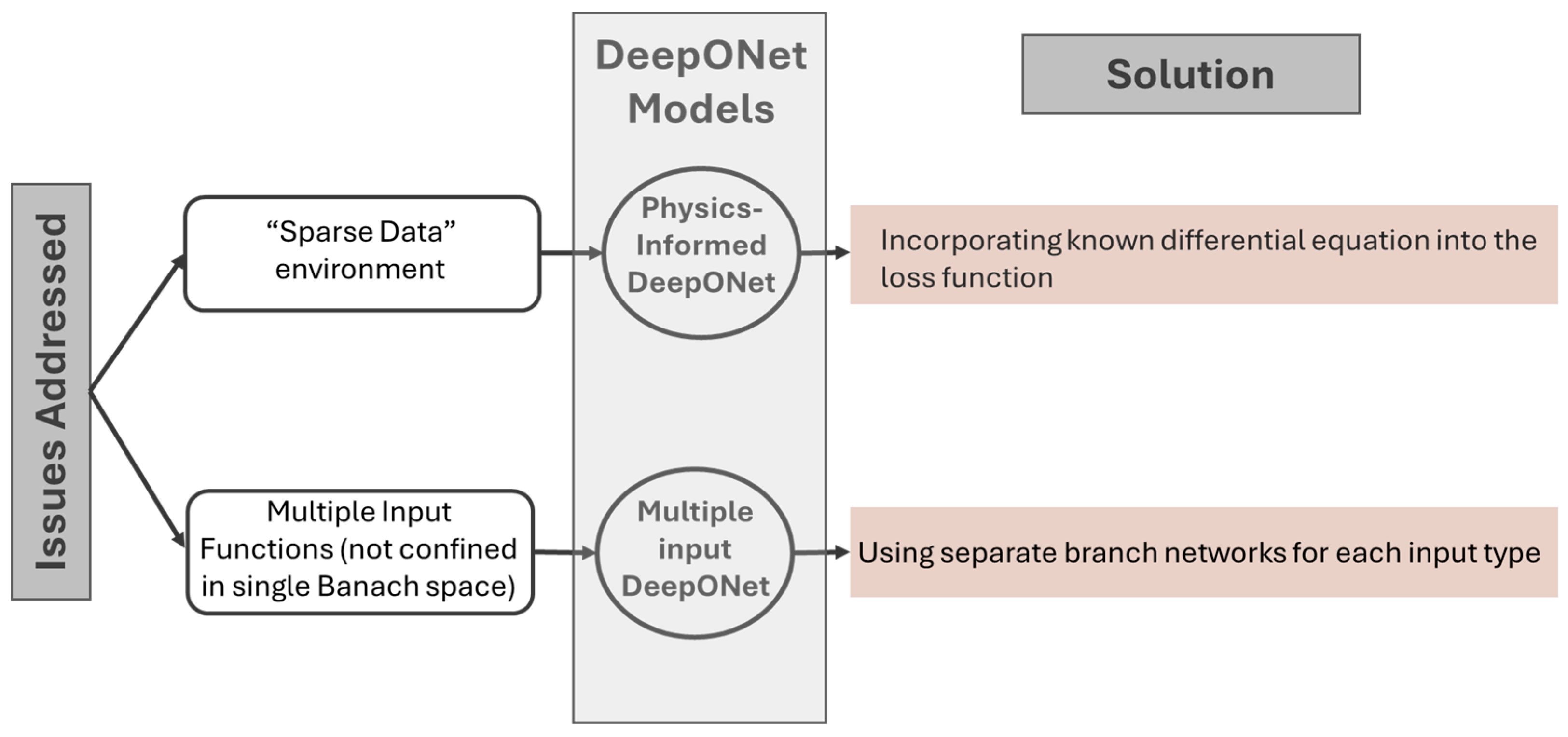
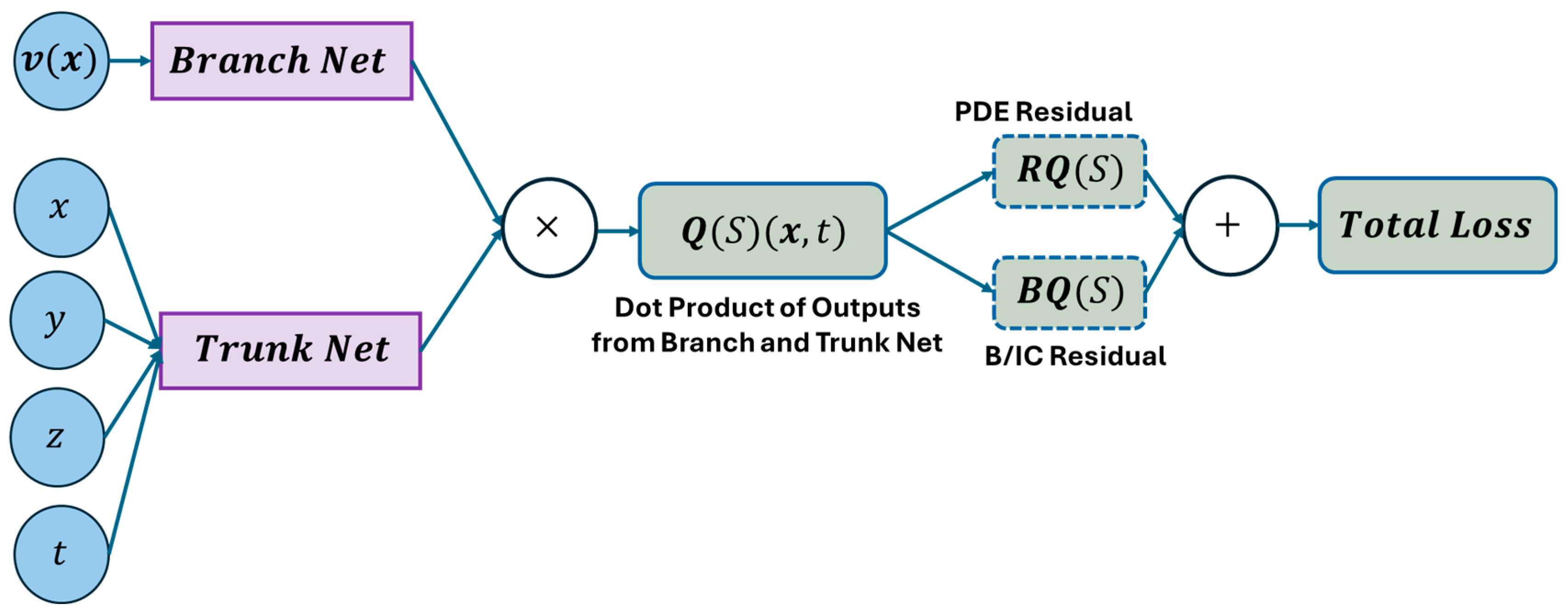
2.2. DeepONet
| Algorithm 1 DeepONet |
| 1: |
| 2: |
| 3: |
| 4: |
| 5: |
| 6: |
| 7: |
| 8: |
| 9: |
| 10: |
| 11: else |
| 12: |
| 13: end if |
| 14: |
| 15: end for |
| 16: end for |
2.3. Physical Understanding of DeepONet
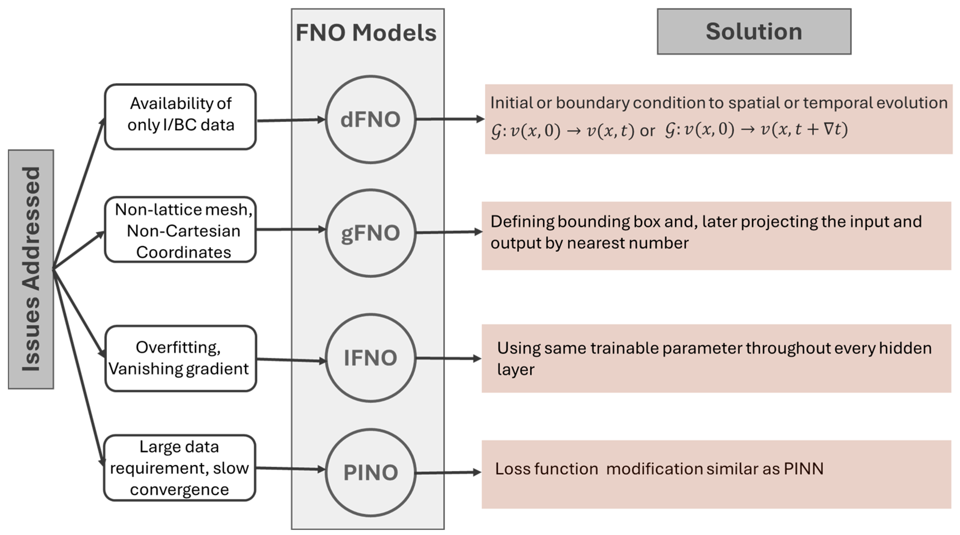
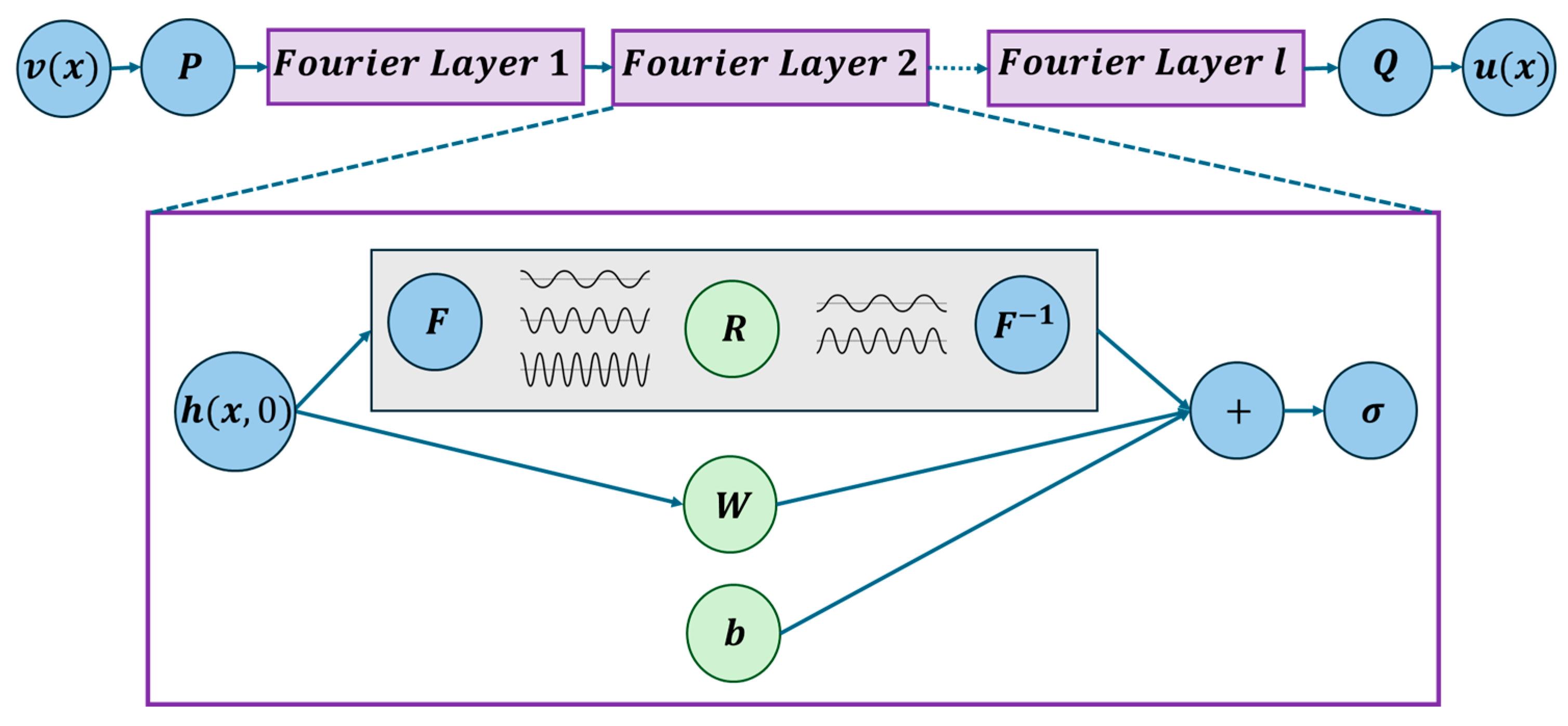
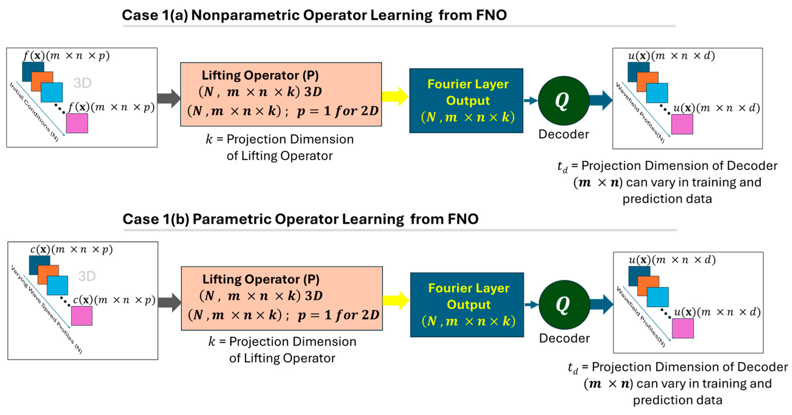
2.4. Fourier Neural Operator (FNO)
| Algorithm 2 FNO |
| 1: |
| 2: |
| 3: |
| 4: |
| 5: |
| 6: |
| 7: |
| 8: end for |
| 9: |
| 10: |
| 11: |
| 12: end for |
| 13: end for |
2.5. Physical Understanding of FNOs
2.6. Application Cases of FNO
3. NO Applications in Wave Propagation
3.1. Wave Propagation with DeepONet
3.2. Wave Propagation with FNOs
4. Conclusions
Author Contributions
Funding
Acknowledgments
Conflicts of Interest
References
- Pant, S.; Laliberte, J.; Martinez, M. Structural Health Monitoring (SHM) of composite aerospace structures using Lamb waves. In Proceedings of the Conference: ICCM19—The 19th International Conference on Composite Materials, Montréal, QC, Canada, 28 July–2 August 2013. [Google Scholar]
- Rocha, H.; Semprimoschnig, C.; Nunes, J.P. Sensors for process and structural health monitoring of aerospace composites: A review. Eng. Struct. 2021, 237, 112231. [Google Scholar] [CrossRef]
- Feng, D.; Feng, M.Q. Computer vision for SHM of civil infrastructure: From dynamic response measurement to damage detection—A review. Eng. Struct. 2018, 156, 105–117. [Google Scholar] [CrossRef]
- Barski, M.; Kędziora, P.; Muc, A.; Romanowicz, P. Structural health monitoring (SHM) methods in machine design and operation. Arch. Mech. Eng. 2014, 61, 653–677. [Google Scholar] [CrossRef]
- Mondoro, A.; Soliman, M.; Frangopol, D.M. Prediction of structural response of naval vessels based on available structural health monitoring data. Ocean Eng. 2016, 125, 295–307. [Google Scholar] [CrossRef]
- Sabra, K.G.; Huston, S. Passive structural health monitoring of a high-speed naval ship from ambient vibrations. J. Acoust. Soc. Am. 2011, 129, 2991–2999. [Google Scholar] [CrossRef]
- Sielski, R.A. Ship structural health monitoring research at the Office of Naval Research. JOM 2012, 64, 823–827. [Google Scholar] [CrossRef]
- Farrar, C.R.; Worden, K. Structural Health Monitoring: A Machine Learning Perspective; John Wiley & Sons: Hoboken, NJ, USA, 2012. [Google Scholar]
- Mitra, M.; Gopalakrishnan, S. Guided wave based structural health monitoring: A review. Smart Mater. Struct. 2016, 25, 053001. [Google Scholar] [CrossRef]
- Farrar, C.R.; Worden, K. An introduction to structural health monitoring. Philos. Trans. R. Soc. A Math. Phys. Eng. Sci. 2007, 365, 303–315. [Google Scholar] [CrossRef]
- Yang, Z.; Yang, H.; Tian, T.; Deng, D.; Hu, M.; Ma, J.; Gao, D.; Zhang, J.; Ma, S.; Yang, L. A review on guided-ultrasonic-wave-based structural health monitoring: From fundamental theory to machine learning techniques. Ultrasonics 2023, 133, 107014. [Google Scholar] [CrossRef]
- Willberg, C.; Duczek, S.; Vivar-Perez, J.M.; Ahmad, Z.A. Simulation methods for guided wave-based structural health monitoring: A review. Appl. Mech. Rev. 2015, 67, 010803. [Google Scholar] [CrossRef]
- Abbas, M.; Shafiee, M. Structural health monitoring (SHM) and determination of surface defects in large metallic structures using ultrasonic guided waves. Sensors 2018, 18, 3958. [Google Scholar] [CrossRef] [PubMed]
- Memmolo, V.; Monaco, E.; Boffa, N.; Maio, L.; Ricci, F. Guided wave propagation and scattering for structural health monitoring of stiffened composites. Compos. Struct. 2018, 184, 568–580. [Google Scholar] [CrossRef]
- Sun, Z.; Rocha, B.; Wu, K.-T.; Mrad, N. A methodological review of piezoelectric based acoustic wave generation and detection techniques for structural health monitoring. Int. J. Aerosp. Eng. 2013, 2013, 928627. [Google Scholar] [CrossRef]
- Light, G. Nondestructive evaluation technologies for monitoring corrosion. In Techniques for Corrosion Monitoring; Elsevier: Amsterdam, The Netherlands, 2021; pp. 285–304. [Google Scholar]
- Viktorov, I.A. Rayleigh Lamb Waves; Springer: Berlin/Heidelberg, Germany, 1967; p. 113. [Google Scholar]
- Länge, K.; Rapp, B.E.; Rapp, M. Surface acoustic wave biosensors: A review. Anal. Bioanal. Chem. 2008, 391, 1509–1519. [Google Scholar] [CrossRef]
- Ding, X.; Li, P.; Lin, S.-C.S.; Stratton, Z.S.; Nama, N.; Guo, F.; Slotcavage, D.; Mao, X.; Shi, J.; Costanzo, F. Surface acoustic wave microfluidics. Lab Chip 2013, 13, 3626–3649. [Google Scholar] [CrossRef]
- Mandal, D.; Banerjee, S. Surface acoustic wave (SAW) sensors: Physics, materials, and applications. Sensors 2022, 22, 820. [Google Scholar] [CrossRef]
- Frye, G.C.; Martin, S.J. Materials characterization using surface acoustic wave devices. Appl. Spectrosc. Rev. 1991, 26, 73–149. [Google Scholar] [CrossRef]
- Hess, P. Surface acoustic waves in materials science. Phys. Today 2002, 55, 42–47. [Google Scholar] [CrossRef]
- Ham, S.; Bathe, K.-J. A finite element method enriched for wave propagation problems. Comput. Struct. 2012, 94, 1–12. [Google Scholar] [CrossRef]
- Moser, F.; Jacobs, L.J.; Qu, J. Modeling elastic wave propagation in waveguides with the finite element method. Ndt E Int. 1999, 32, 225–234. [Google Scholar] [CrossRef]
- Ha, S.; Chang, F.-K. Optimizing a spectral element for modeling PZT-induced Lamb wave propagation in thin plates. Smart Mater. Struct. 2009, 19, 015015. [Google Scholar] [CrossRef]
- Ge, L.; Wang, X.; Wang, F. Accurate modeling of PZT-induced Lamb wave propagation in structures by using a novel spectral finite element method. Smart Mater. Struct. 2014, 23, 095018. [Google Scholar] [CrossRef]
- Zou, F.; Aliabadi, M. On modelling three-dimensional piezoelectric smart structures with boundary spectral element method. Smart Mater. Struct. 2017, 26, 055015. [Google Scholar] [CrossRef]
- Balasubramanyam, R.; Quinney, D.; Challis, R.; Todd, C. A finite-difference simulation of ultrasonic Lamb waves in metal sheets with experimental verification. J. Phys. D Appl. Phys. 1996, 29, 147. [Google Scholar] [CrossRef]
- Cho, Y.; Rose, J.L. A boundary element solution for a mode conversion study on the edge reflection of Lamb waves. J. Acoust. Soc. Am. 1996, 99, 2097–2109. [Google Scholar] [CrossRef]
- Yim, H.; Sohn, Y. Numerical simulation and visualization of elastic waves using mass-spring lattice model. IEEE Trans. Ultrason. Ferroelectr. Freq. Control 2000, 47, 549–558. [Google Scholar]
- Bergamini, A.; Biondini, F. Finite strip modeling for optimal design of prestressed folded plate structures. Eng. Struct. 2004, 26, 1043–1054. [Google Scholar] [CrossRef]
- Diehl, P.; Schweitzer, M.A. Simulation of wave propagation and impact damage in brittle materials using peridynamics. In Recent Trends in Computational Engineering-CE2014; Springer: Cham, Switzerland, 2015; pp. 251–265. [Google Scholar]
- Rahman, F.M.M.; Banerjee, S. Peri-elastodynamic: Peridynamic simulation method for guided waves in materials. Mech. Syst. Signal Process. 2024, 219, 111560. [Google Scholar] [CrossRef]
- Nishawala, V.V.; Ostoja-Starzewski, M.; Leamy, M.J.; Demmie, P.N. Simulation of elastic wave propagation using cellular automata and peridynamics, and comparison with experiments. Wave Motion 2016, 60, 73–83. [Google Scholar] [CrossRef]
- Kluska, P.; Staszewski, W.; Leamy, M.; Uhl, T. Cellular automata for Lamb wave propagation modelling in smart structures. Smart Mater. Struct. 2013, 22, 085022. [Google Scholar] [CrossRef]
- Leckey, C.A.; Rogge, M.D.; Miller, C.A.; Hinders, M.K. Multiple-mode Lamb wave scattering simulations using 3D elastodynamic finite integration technique. Ultrasonics 2012, 52, 193–207. [Google Scholar] [CrossRef] [PubMed]
- McEneaney, W.M. A curse-of-dimensionality-free numerical method for solution of certain HJB PDEs. SIAM J. Control Optim. 2007, 46, 1239–1276. [Google Scholar] [CrossRef]
- Connell, K.O.; Cashman, A. Development of a numerical wave tank with reduced discretization error. In Proceedings of the 2016 International Conference on Electrical, Electronics, and Optimization Techniques (ICEEOT), Chennai, India, 3–5 March 2016; IEEE: Piscataway, NJ, USA, 2016; pp. 3008–3012. [Google Scholar]
- Biondini, G.; Trogdon, T. Gibbs phenomenon for dispersive PDEs. arXiv 2015, arXiv:1411.6142. [Google Scholar] [CrossRef]
- Bernardi, C.; Maday, Y. Spectral methods. In Handbook of Numerical Analysis; Elsevier: Amsterdam, The Netherlands, 1997. [Google Scholar]
- Shizgal, B.D.; Jung, J.-H. Towards the resolution of the Gibbs phenomena. J. Comput. Appl. Math. 2003, 161, 41–65. [Google Scholar] [CrossRef]
- Banerjee, S.; Leckey, C.A. Computational Nondestructive Evaluation Handbook: Ultrasound Modeling Techniques; CRC Press: Boca Raton, FL, USA, 2020. [Google Scholar]
- Rahani, E.K.; Kundu, T. Gaussian-DPSM (G-DPSM) and Element Source Method (ESM) modifications to DPSM for ultrasonic field modeling. Ultrasonics 2011, 51, 625–631. [Google Scholar] [CrossRef]
- Monaco, E.; Rautela, M.; Gopalakrishnan, S.; Ricci, F. Machine learning algorithms for delaminations detection on composites panels by wave propagation signals analysis: Review, experiences and results. Prog. Aerosp. Sci. 2024, 146, 100994. [Google Scholar] [CrossRef]
- Cantero-Chinchilla, S.; Wilcox, P.D.; Croxford, A.J. Deep learning in automated ultrasonic NDE–developments, axioms and opportunities. Ndt E Int. 2022, 131, 102703. [Google Scholar] [CrossRef]
- Carleo, G.; Cirac, I.; Cranmer, K.; Daudet, L.; Schuld, M.; Tishby, N.; Vogt-Maranto, L.; Zdeborová, L. Machine learning and the physical sciences. Rev. Mod. Phys. 2019, 91, 045002. [Google Scholar] [CrossRef]
- Cuomo, S.; Di Cola, V.S.; Giampaolo, F.; Rozza, G.; Raissi, M.; Piccialli, F. Scientific machine learning through physics–informed neural networks: Where we are and what’s next. J. Sci. Comput. 2022, 92, 88. [Google Scholar] [CrossRef]
- Hey, T.; Butler, K.; Jackson, S.; Thiyagalingam, J. Machine learning and big scientific data. Philos. Trans. R. Soc. A 2020, 378, 20190054. [Google Scholar] [CrossRef]
- Takamoto, M.; Praditia, T.; Leiteritz, R.; MacKinlay, D.; Alesiani, F.; Pflüger, D.; Niepert, M. Pdebench: An extensive benchmark for scientific machine learning. Adv. Neural Inf. Process. Syst. 2022, 35, 1596–1611. [Google Scholar]
- Thiyagalingam, J.; Shankar, M.; Fox, G.; Hey, T. Scientific machine learning benchmarks. Nat. Rev. Phys. 2022, 4, 413–420. [Google Scholar] [CrossRef]
- Li, Y.; Zhang, X.; Cheng, L.; Xie, M.; Cao, K. 3D wave simulation based on a deep learning model for spatiotemporal prediction. Ocean Eng. 2022, 263, 112420. [Google Scholar] [CrossRef]
- Moseley, B.; Markham, A.; Nissen-Meyer, T. Solving the wave equation with physics-informed deep learning. arXiv 2020, arXiv:2006.11894. [Google Scholar]
- Daoud, M.S.; Shehab, M.; Al-Mimi, H.M.; Abualigah, L.; Zitar, R.A.; Shambour, M.K.Y. Gradient-based optimizer (GBO): A review, theory, variants, and applications. Arch. Comput. Methods Eng. 2023, 30, 2431–2449. [Google Scholar] [CrossRef]
- Haji, S.H.; Abdulazeez, A.M. Comparison of optimization techniques based on gradient descent algorithm: A review. PalArch’s J. Archaeol. Egypt/Egyptol. 2021, 18, 2715–2743. [Google Scholar]
- Karimpouli, S.; Tahmasebi, P. Physics informed machine learning: Seismic wave equation. Geosci. Front. 2020, 11, 1993–2001. [Google Scholar] [CrossRef]
- Kim, Y.; Nakata, N. Geophysical inversion versus machine learning in inverse problems. Lead. Edge 2018, 37, 894–901. [Google Scholar] [CrossRef]
- Smaragdakis, C.; Taroudaki, V.; Taroudakis, M.I. Using machine learning techniques in inverse problems of acoustical oceanography. Stud. Appl. Math. 2024, 153, e12704. [Google Scholar] [CrossRef]
- Faroughi, S.A.; Pawar, N.M.; Fernandes, C.; Raissi, M.; Das, S.; Kalantari, N.K.; Kourosh Mahjour, S. Physics-guided, physics-informed, and physics-encoded neural networks and operators in scientific computing: Fluid and solid mechanics. J. Comput. Inf. Sci. Eng. 2024, 24, 040802. [Google Scholar] [CrossRef]
- Mehtaj, N.; Banerjee, S. Scientific Machine Learning for Guided Wave and Surface Acoustic Wave (SAW) Propagation: PgNN, PeNN, PINN, and Neural Operator. Sensors 2025, 25, 1401. [Google Scholar] [CrossRef] [PubMed]
- Jia, J.; Li, Y. Deep learning for structural health monitoring: Data, algorithms, applications, challenges, and trends. Sensors 2023, 23, 8824. [Google Scholar] [CrossRef] [PubMed]
- Capineri, L.; Bulletti, A. Ultrasonic guided-waves sensors and integrated structural health monitoring systems for impact detection and localization: A review. Sensors 2021, 21, 2929. [Google Scholar] [CrossRef]
- Eltouny, K.; Gomaa, M.; Liang, X. Unsupervised learning methods for data-driven vibration-based structural health monitoring: A review. Sensors 2023, 23, 3290. [Google Scholar] [CrossRef] [PubMed]
- Flah, M.; Nunez, I.; Ben Chaabene, W.; Nehdi, M.L. Machine learning algorithms in civil structural health monitoring: A systematic review. Arch. Comput. Methods Eng. 2021, 28, 2621–2643. [Google Scholar] [CrossRef]
- Gomez-Cabrera, A.; Escamilla-Ambrosio, P.J. Review of machine-learning techniques applied to structural health monitoring systems for building and bridge structures. Appl. Sci. 2022, 12, 10754. [Google Scholar] [CrossRef]
- Yuan, F.-G.; Zargar, S.A.; Chen, Q.; Wang, S. Machine learning for structural health monitoring: Challenges and opportunities. In Sensors and Smart Structures Technologies for Civil, Mechanical, and Aerospace Systems 2020; SPIE Digital Library: Bellingham, WA, USA, 2020; Volume 11379, p. 1137903. [Google Scholar]
- Raissi, M.; Perdikaris, P.; Karniadakis, G.E. Physics-informed neural networks: A deep learning framework for solving forward and inverse problems involving nonlinear partial differential equations. J. Comput. Phys. 2019, 378, 686–707. [Google Scholar] [CrossRef]
- Rao, C.; Ren, P.; Liu, Y.; Sun, H. Discovering nonlinear PDEs from scarce data with physics-encoded learning. arXiv 2022, arXiv:2201.12354. [Google Scholar]
- Rao, C.; Ren, P.; Wang, Q.; Buyukozturk, O.; Sun, H.; Liu, Y. Encoding physics to learn reaction–diffusion processes. Nat. Mach. Intell. 2023, 5, 765–779. [Google Scholar] [CrossRef]
- Rao, C.; Sun, H.; Liu, Y. Hard encoding of physics for learning spatiotemporal dynamics. arXiv 2021, arXiv:2105.00557. [Google Scholar]
- Li, W.; Bazant, M.Z.; Zhu, J. A physics-guided neural network framework for elastic plates: Comparison of governing equations-based and energy-based approaches. Comput. Methods Appl. Mech. Eng. 2021, 383, 113933. [Google Scholar] [CrossRef]
- Brunton, S.L.; Proctor, J.L.; Kutz, J.N. Discovering governing equations from data by sparse identification of nonlinear dynamical systems. Proc. Natl. Acad. Sci. USA 2016, 113, 3932–3937. [Google Scholar] [CrossRef] [PubMed]
- Cybenko, G. Approximation by superpositions of a sigmoidal function. Math. Control Signals Syst. 1989, 2, 303–314. [Google Scholar] [CrossRef]
- Funahashi, K.-I. On the approximate realization of continuous mappings by neural networks. Neural Netw. 1989, 2, 183–192. [Google Scholar] [CrossRef]
- Hornik, K.; Stinchcombe, M.; White, H. Multilayer feedforward networks are universal approximators. Neural Netw. 1989, 2, 359–366. [Google Scholar] [CrossRef]
- Boullé, N.; Townsend, A. A mathematical guide to operator learning. arXiv 2023, arXiv:2312.14688. [Google Scholar]
- Maier, A.; Köstler, H.; Heisig, M.; Krauss, P.; Yang, S.H. Known operator learning and hybrid machine learning in medical imaging—A review of the past, the present, and the future. Prog. Biomed. Eng. 2022, 4, 022002. [Google Scholar] [CrossRef]
- Chen, T.; Chen, H. Universal approximation to nonlinear operators by neural networks with arbitrary activation functions and its application to dynamical systems. IEEE Trans. Neural Netw. 1995, 6, 911–917. [Google Scholar] [CrossRef]
- Kovachki, N.; Li, Z.; Liu, B.; Azizzadenesheli, K.; Bhattacharya, K.; Stuart, A.; Anandkumar, A. Neural operator: Learning maps between function spaces with applications to pdes. J. Mach. Learn. Res. 2023, 24, 1–97. [Google Scholar]
- Lu, L.; Jin, P.; Pang, G.; Zhang, Z.; Karniadakis, G.E. Learning nonlinear operators via DeepONet based on the universal approximation theorem of operators. Nat. Mach. Intell. 2021, 3, 218–229. [Google Scholar] [CrossRef]
- Li, Z.; Kovachki, N.; Azizzadenesheli, K.; Liu, B.; Bhattacharya, K.; Stuart, A.; Anandkumar, A. Fourier neural operator for parametric partial differential equations. arXiv 2020, arXiv:2010.08895. [Google Scholar]
- Tripura, T.; Chakraborty, S. Wavelet neural operator: A neural operator for parametric partial differential equations. arXiv 2022, arXiv:2205.02191. [Google Scholar]
- Cao, Q.; Goswami, S.; Karniadakis, G.E. Laplace neural operator for solving differential equations. Nat. Mach. Intell. 2024, 6, 631–640. [Google Scholar] [CrossRef]
- Raonic, B.; Molinaro, R.; Rohner, T.; Mishra, S.; de Bezenac, E. Convolutional neural operators. In Proceedings of the ICLR 2023 Workshop on Physics for Machine Learning, Kigali, Rwanda, 4 May 2023. [Google Scholar]
- Fanaskov, V.S.; Oseledets, I.V. Spectral neural operators. Dokl. Math. 2023, 108, S226–S232. [Google Scholar] [CrossRef]
- Goswami, S.; Bora, A.; Yu, Y.; Karniadakis, G.E. Physics-informed deep neural operator networks. In Machine Learning in Modeling and Simulation: Methods and Applications; Springer: Berlin/Heidelberg, Germany, 2023; pp. 219–254. [Google Scholar]
- Cilimkovic, M. Neural Networks and Back Propagation Algorithm; Institute of Technology Blanchardstown: Dublin, Ireland, 2015; Volume 15, p. 18. [Google Scholar]
- Goswami, S.; Yin, M.; Yu, Y.; Karniadakis, G.E. A physics-informed variational DeepONet for predicting crack path in quasi-brittle materials. Comput. Methods Appl. Mech. Eng. 2022, 391, 114587. [Google Scholar] [CrossRef]
- Wang, S.; Wang, H.; Perdikaris, P. Learning the solution operator of parametric partial differential equations with physics-informed DeepONets. Sci. Adv. 2021, 7, eabi8605. [Google Scholar] [CrossRef]
- Jin, P.; Meng, S.; Lu, L. MIONet: Learning multiple-input operators via tensor product. SIAM J. Sci. Comput. 2022, 44, A3490–A3514. [Google Scholar] [CrossRef]
- Tan, L.; Chen, L. Enhanced deeponet for modeling partial differential operators considering multiple input functions. arXiv 2022, arXiv:2202.08942. [Google Scholar]
- Aldirany, Z.; Cottereau, R.; Laforest, M.; Prudhomme, S. Operator approximation of the wave equation based on deep learning of Green’s function. Comput. Math. Appl. 2024, 159, 21–30. [Google Scholar] [CrossRef]
- Hendrycks, D.; Gimpel, K. Gaussian error linear units (gelus). arXiv 2016, arXiv:1606.08415. [Google Scholar]
- Li, Y.; Yuan, Y. Convergence analysis of two-layer neural networks with relu activation. In Proceedings of the Advances in Neural Information Processing Systems 30 (NIPS 2017), Long Beach, CA, USA, 4–9 December 2017; Volume 30. [Google Scholar]
- Zhu, M.; Feng, S.; Lin, Y.; Lu, L. Fourier-DeepONet: Fourier-enhanced deep operator networks for full waveform inversion with improved accuracy, generalizability, and robustness. Comput. Methods Appl. Mech. Eng. 2023, 416, 116300. [Google Scholar] [CrossRef]
- Wen, G.; Li, Z.; Azizzadenesheli, K.; Anandkumar, A.; Benson, S.M. U-FNO—An enhanced Fourier neural operator-based deep-learning model for multiphase flow. Adv. Water Resour. 2022, 163, 104180. [Google Scholar] [CrossRef]
- Guo, Z.; Chai, L.; Huang, S.; Li, Y. Inversion-DeepONet: A Novel DeepONet-Based Network with Encoder-Decoder for Full Waveform Inversion. arXiv 2024, arXiv:2408.08005. [Google Scholar]
- Li, S.; Li, Z.; Mu, Z.; Xin, S.; Dai, Z.; Leng, K.; Zhang, R.; Song, X.; Zhu, Y. GlobalTomo: A global dataset for physics-ML seismic wavefield modeling and FWI. arXiv 2024, arXiv:2406.18202. [Google Scholar]
- Wagner, J.E.; Burbulla, S.; de Benito Delgado, M.; Schmid, J.D. Neural Operators as Fast Surrogate Models for the Transmission Loss of Parameterized Sonic Crystals. In Proceedings of the NeurIPS 2024 Workshop on Data-driven and Differentiable Simulations, Surrogates, and Solvers, Vancouver, BC, Canada, 15 December 2024. [Google Scholar]
- Bao, Y.; Li, H. Machine learning paradigm for structural health monitoring. Struct. Health Monit. 2021, 20, 1353–1372. [Google Scholar] [CrossRef]
- Smarsly, K.; Dragos, K.; Wiggenbrock, J. Machine learning techniques for structural health monitoring. In Proceedings of the 8th European Workshop on Structural Health Monitoring (EWSHM 2016), Bilbao, Spain, 5–8 July 2016; pp. 5–8. [Google Scholar]
- Gubernatis, J.; Lookman, T. Machine learning in materials design and discovery: Examples from the present and suggestions for the future. Phys. Rev. Mater. 2018, 2, 120301. [Google Scholar] [CrossRef]
- Moosavi, S.M.; Jablonka, K.M.; Smit, B. The role of machine learning in the understanding and design of materials. J. Am. Chem. Soc. 2020, 142, 20273–20287. [Google Scholar] [CrossRef]
- Erickson, B.J.; Korfiatis, P.; Akkus, Z.; Kline, T.L. Machine learning for medical imaging. RadioGraphics 2017, 37, 505–515. [Google Scholar] [CrossRef]
- Yang, Y.; Gao, A.F.; Castellanos, J.C.; Ross, Z.E.; Azizzadenesheli, K.; Clayton, R.W. Seismic wave propagation and inversion with neural operators. Seism. Rec. 2021, 1, 126–134. [Google Scholar] [CrossRef]
- Song, C.; Wang, Y. High-frequency wavefield extrapolation using the Fourier neural operator. J. Geophys. Eng. 2022, 19, 269–282. [Google Scholar] [CrossRef]
- Zhang, T.; Innanen, K.; Trad, D. Learning the elastic wave equation with Fourier Neural Operators. Geoconvention 2022, 2022, 1–5. [Google Scholar] [CrossRef]
- Li, B.; Wang, H.; Feng, S.; Yang, X.; Lin, Y. Solving seismic wave equations on variable velocity models with Fourier neural operator. IEEE Trans. Geosci. Remote Sens. 2023, 61, 1–18. [Google Scholar] [CrossRef]
- Lehmann, F.; Gatti, F.; Bertin, M.; Clouteau, D. Fourier neural operator surrogate model to predict 3D seismic waves propagation. arXiv 2023, arXiv:2304.10242. [Google Scholar]
- Kong, Q.; Rodgers, A. Feasibility of Using Fourier Neural Operators for 3D Elastic Seismic Simulations; Lawrence Livermore National Laboratory (LLNL): Livermore, CA, USA, 2023.
- Middleton, M.; Murphy, D.T.; Savioja, L. The application of Fourier neural operator networks for solving the 2D linear acoustic wave equation. In Forum Acusticum; European Acoustics Association: Turin, Italy, 2023. [Google Scholar]
- Rosofsky, S.G.; Al Majed, H.; Huerta, E. Applications of physics informed neural operators. Mach. Learn. Sci. Technol. 2023, 4, 025022. [Google Scholar] [CrossRef]
- Konuk, T.; Shragge, J. Physics-guided deep learning using fourier neural operators for solving the acoustic VTI wave equation. In Proceedings of the 82nd EAGE Annual Conference & Exhibition, Amsterdam, The Netherlands, 18–21 October 2021; European Association of Geoscientists & Engineers: Utrecht, The Netherlands, 2021. [Google Scholar]
- Guan, S.; Hsu, K.-T.; Chitnis, P.V. Fourier neural operator network for fast photoacoustic wave simulations. Algorithms 2023, 16, 124. [Google Scholar] [CrossRef]


| Aspects | DeepONet | FNO |
|---|---|---|
| Operator type | Approximates via finite basis expansion | Approximates via Fourier-domain convolution |
| Kernel function | Implicit via trunk net basis and branch net coefficients | Explicit via learned Fourier multipliers |
| Integral approximation | Discrete latent expansion into number of modes and their contributions | Fourier transform, multiply in spectral space |
| Global modeling | Through learned basis functions in trunk net | Through Fourier modes capturing global functional behavior |
| Miscellaneous understanding | Very general; works for arbitrary operators | Most efficient when operator is translation-invariant (convolution-like PDEs) |
| Parametric PDEs | Yes Input: Parametric function (e.g., wave speed map , initial profile) | Yes Input: Parametric function (e.g., wave speed map , initial profile) |
| Nonparametric PDEs | Yes Input: Prior field value (e.g., ) | Yes Input: Prior field value (e.g., ) |
| Inverse Problem | No: tough to converge | Yes |
| Authors | Year | Key Objectives | Model Architecture | Type of Wave | Dimension | Type of Medium |
|---|---|---|---|---|---|---|
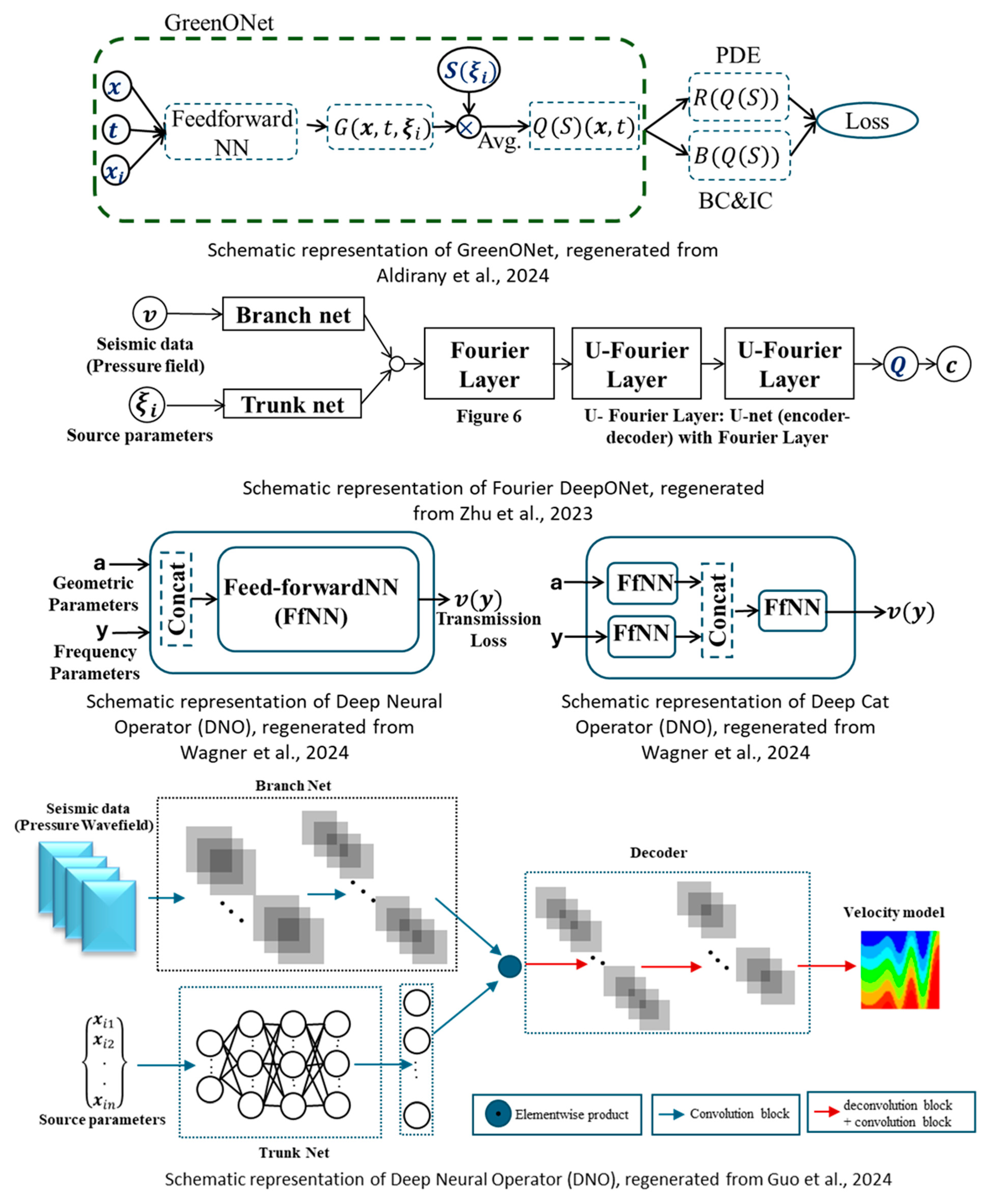
| Aldirany et al. [91] | 2024 | Transient wave propagation modeling | DeepONet and GreenONet | Acoustic wave | 2D | Homogeneous |
| Zhu et al. [94] | 2024 | Full waveform inversion with noise-robust generalization | Fourier DeepONet | Acoustic wave | 2D | Heterogeneous |
| Guo et al. [96] | 2024 | Improve generalization across source locations and frequencies | Inversion DeepONet | Acoustic wave | 2D | Heterogeneous |
| Li et al. [97] | 2024 | Accelerated global seismic forward modeling and inversion | DeepONet, Physics-Informed DeepONet | Acoustic wave and Elastic wave | 3D | Heterogeneous |
| Wagner et al. [98] | 2023 | Fast surrogate modeling of transmission loss in sonic crystals | DeepONet | Acoustic wave | 2D | Homogeneous |
| Authors | Year | Key Objectives | Model Architecture | Type of Wave | Dimension | Type of Medium |
|---|---|---|---|---|---|---|
| Yang et al. [104] | 2021 | Fast inference of 2D seismic wavefields across varying source and velocity | Vanilla FNO | Acoustic wave | 2D | Heterogeneous |
| Song and Yang [105] | 2022 | Predicting high-frequency wavefields from low-frequency inputs | Vanilla FNO | Acoustic wave | 2D | Heterogeneous |
| Zhang et al. [106] | 2022 | Time extrapolation of wavefields for seismic analysis | Vanilla FNO | Elastic wave | 2D | Heterogeneous |
| Li et al. [107] | 2023 | Forward modeling across diverse velocity models for full waveform inversion | Parallel FNO (PFNO) | Acoustic wave | 2D | Heterogeneous |
| Lehmann et al. [108] | 2023 | Simulating 3D elastic ground motion for earthquake hazard assessment | U-Shaped FNO (UNO) | Elastic wave | 3D | Heterogeneous |
| Kong et al. [109] | 2023 | Real-time simulation of 3D ground motion for subsurface imaging and seismic inversion | UNO and Vanilla FNO | Elastic wave | 3D | Homogeneous |
| Middleton et al. [110] | 2023 | Learning long-term acoustic wave propagation from short input in a free-field simulation | Tensorized FNO (TFNO) | Acoustic wave | 2D | Homogeneous |
| Rosofsky et al. [111] | 2023 | Surrogate modeling of wave equation | Physics-Informed FNO (PIFNO) | Elastic wave | 1D, 2D | Homogeneous |
| Konuk and Shragge [112] | 2023 | Generalizing frequency domain AWE solutions for anisotropic media across frequencies | PIFNO | Acoustic wave | 2D | Anisotropic VTI |
| Guan et al. [113] | 2023 | Fast modeling of broadband photoacoustic wave propagation for image reconstruction applications | Vanilla FNO | Acoustic waves | 2D | Homogeneous |
Disclaimer/Publisher’s Note: The statements, opinions and data contained in all publications are solely those of the individual author(s) and contributor(s) and not of MDPI and/or the editor(s). MDPI and/or the editor(s) disclaim responsibility for any injury to people or property resulting from any ideas, methods, instructions or products referred to in the content. |
© 2025 by the authors. Licensee MDPI, Basel, Switzerland. This article is an open access article distributed under the terms and conditions of the Creative Commons Attribution (CC BY) license (https://creativecommons.org/licenses/by/4.0/).
Share and Cite
Mehtaj, N.; Banerjee, S. Scientific Machine Learning for Elastic and Acoustic Wave Propagation: Neural Operator and Physics-Guided Neural Network. Sensors 2025, 25, 3588. https://doi.org/10.3390/s25123588
Mehtaj N, Banerjee S. Scientific Machine Learning for Elastic and Acoustic Wave Propagation: Neural Operator and Physics-Guided Neural Network. Sensors. 2025; 25(12):3588. https://doi.org/10.3390/s25123588
Chicago/Turabian StyleMehtaj, Nafisa, and Sourav Banerjee. 2025. "Scientific Machine Learning for Elastic and Acoustic Wave Propagation: Neural Operator and Physics-Guided Neural Network" Sensors 25, no. 12: 3588. https://doi.org/10.3390/s25123588
APA StyleMehtaj, N., & Banerjee, S. (2025). Scientific Machine Learning for Elastic and Acoustic Wave Propagation: Neural Operator and Physics-Guided Neural Network. Sensors, 25(12), 3588. https://doi.org/10.3390/s25123588