
Portable Impedance Analyzer for FET-Based Biosensors with Embedded Analysis of Randles Circuits’ Spectra

 , , , ,
  ,
,  and
and
Abstract

1. Introduction
2. Materials and Methods
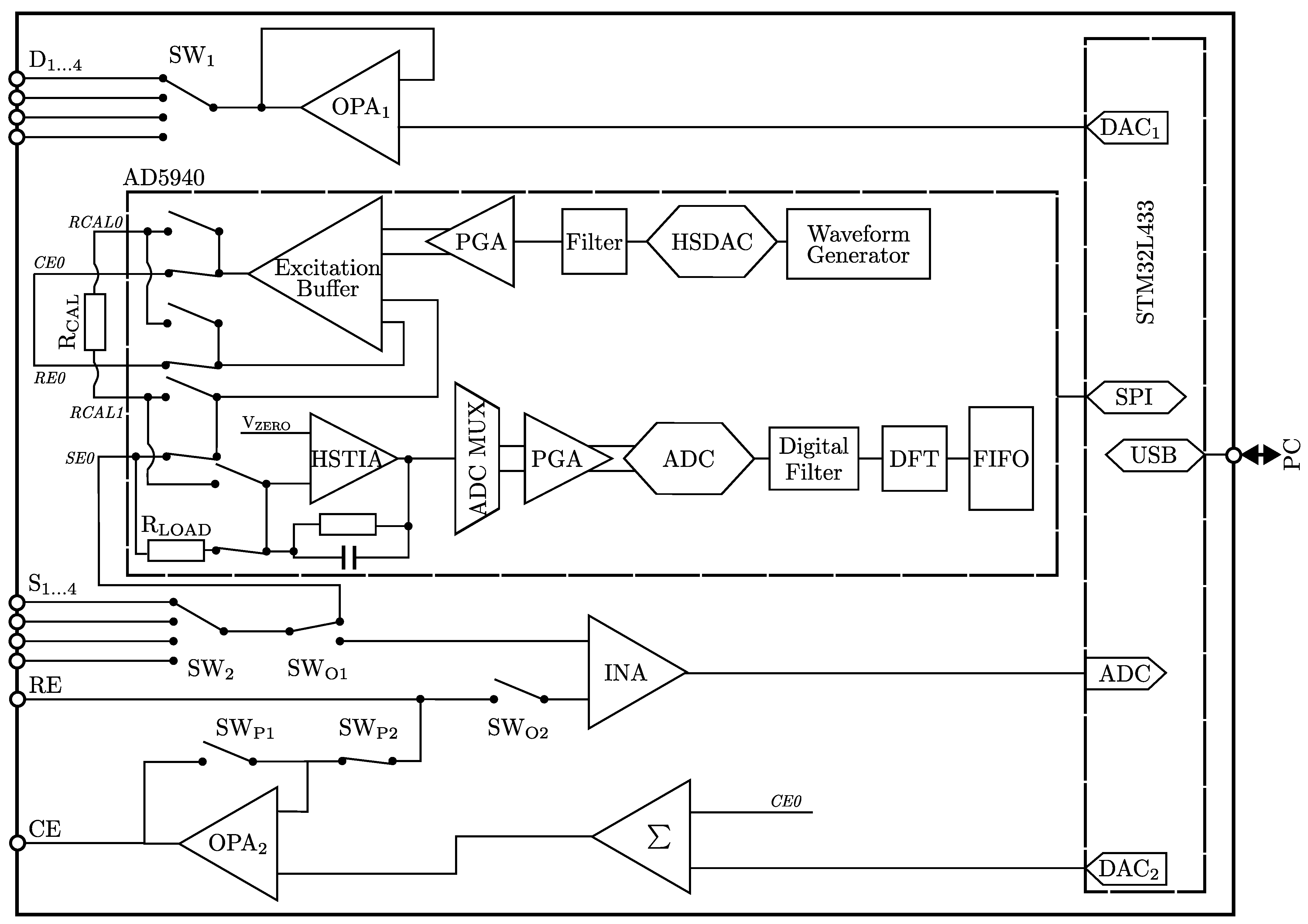
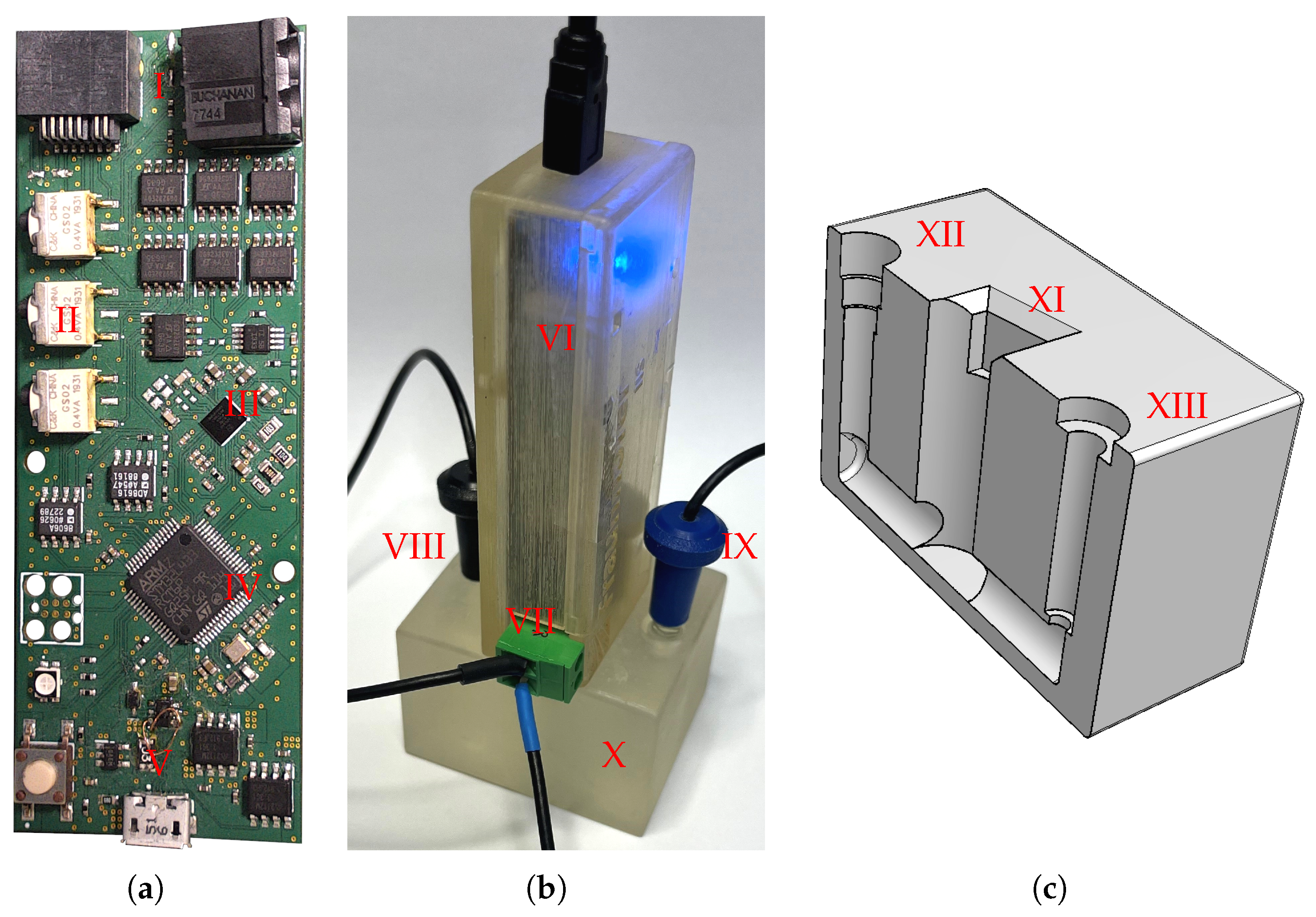
2.1. Portable Impedance Analyzer
2.2. Fitting Algorithm
2.3. Test Data Set
2.4. Randles Circruit Simulator
2.5. Real-World Tests with ISFETs
3. Results
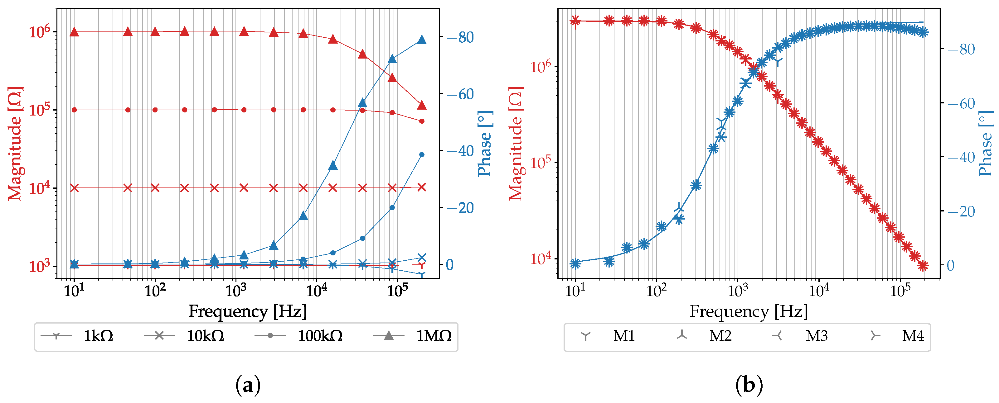
3.1. Evaluation of the PIA
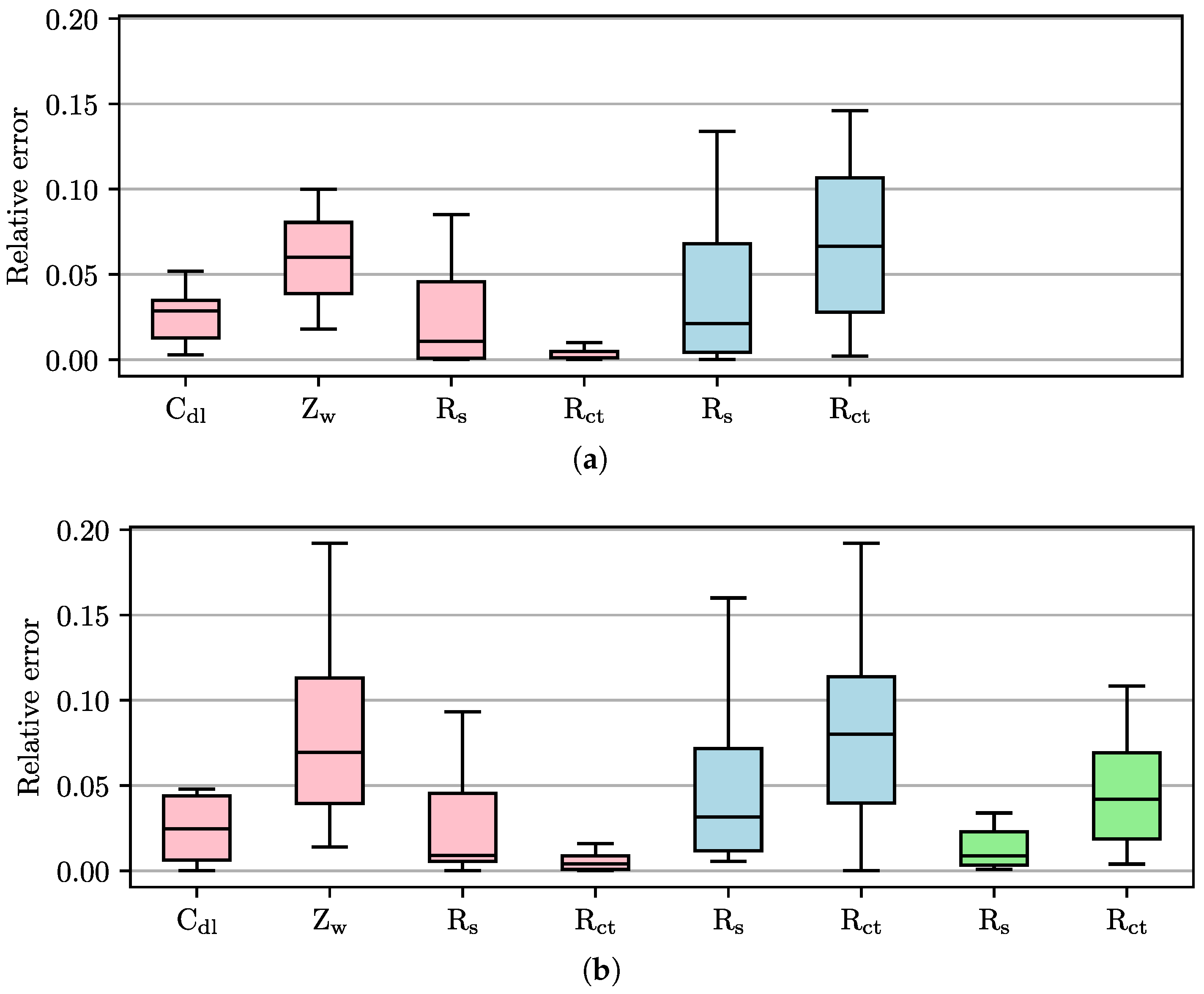
3.2. Accuracy and Robustness of Circular Fitting
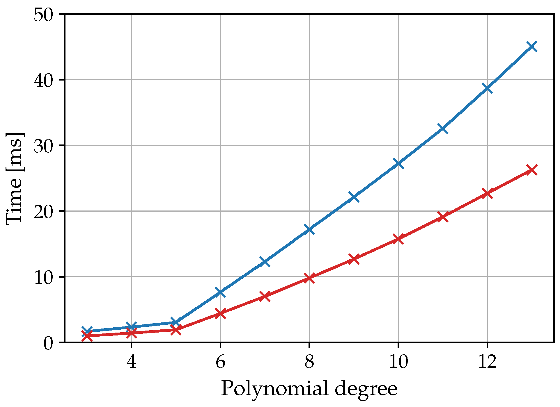
3.3. Computing Effort of the Circular Fitting on the Embedded System
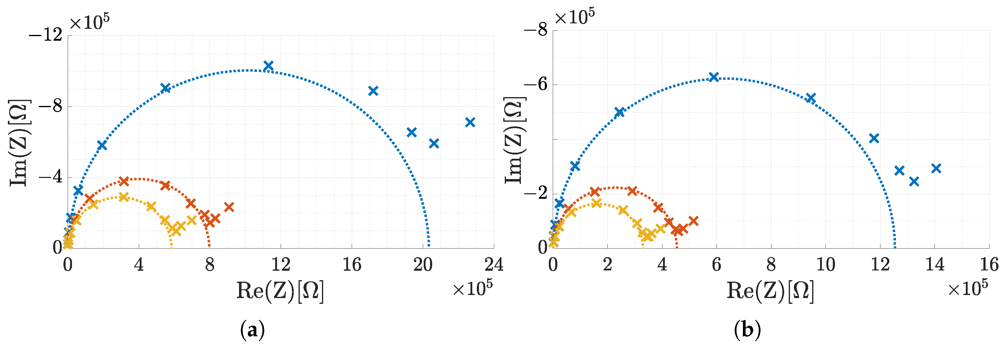
3.4. Real-World Tests with ISFETs
4. Discussion and Conclusions
Supplementary Materials
Author Contributions
Funding
Data Availability Statement
Conflicts of Interest
Abbreviations
| AC | Alternating current |
| ADC | Analog-to-digital converter |
| AFE | Analog front end |
| BioFET | Field-effect transistor-based biosensor |
| BLE | Bluetooth low energy |
| CE | Counter electrode |
| CNLS | Complex non-linear least squares |
| CPE | Constant phase element |
| DAC | Digital-to-analog converter |
| DC | Direct current |
| DFT | Discrete fourier transform |
| DMA | Direct memory access |
| DNA | Deoxyribonucleic acid |
| ECD | Equivalent circuit diagram |
| EIS | Electrochemical impedance spectroscopy |
| FET | Field effect transistor |
| FIFO | First-in-first-out |
| GUI | Graphical user interface |
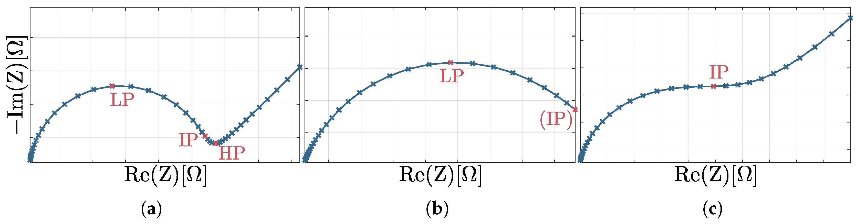
| HP | High point |
| HSDAC | High speed digital-to-analog converter |
| HSTIA | High speed transimpedance amplifier |
| INA | Instrumentation amplifier |
| IoT | Internet of things |
| IP | Inflection point |
| IQR | Interquartil range |
| ISFET | Ion-sensitive field-effect transistor |
| LP | Low point |
| OCV | Open-circuit voltage |
| OPA | Operational amplifier |
| PC | Personal computer |
| PCB | Printed circuit board |
| PGA | Programmable gain amplifier |
| PIA | Portable impedance analyzer |
| POC | Point of care |
| QINIPE | Quadratic interpolation non-iterative parameter estimation |
| RCS | Randles circuit simulator |
| RE | Reference electrode |
| RMSRE | Root mean squared relative error |
| SysTick | System tick time |
| TIA | Transimpedance amplifier |
| UART | Universal asynchronous receiver/transmitter |
| USB | Universal serial bus |
| WE | Working electrode |
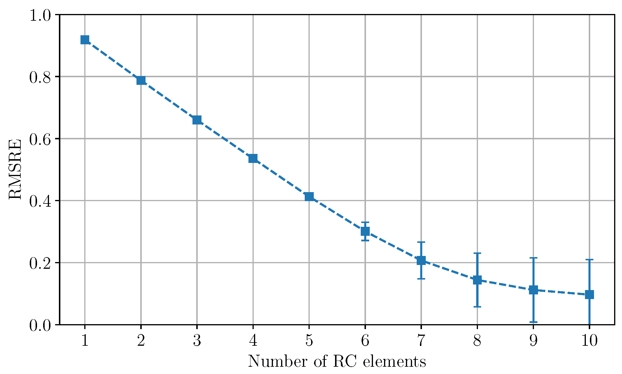
Appendix A. Number of RC Elements for the Simulation of ZW
References
- Tu, J.; Torrente-Rodríguez, R.M.; Wang, M.; Gao, W. The Era of Digital Health: A Review of Portable and Wearable Affinity Biosensors. Adv. Funct. Mater. 2020, 30, 1906713. [Google Scholar] [CrossRef]
- Gavrilas, S.; Ursachi, C.S.; Perța-Crisan, S.; Munteanu, F.D. Recent Trends in Biosensors for Environmental Quality Monitoring. Sensors 2022, 22, 1513. [Google Scholar] [CrossRef] [PubMed]
- Ferrari, A.G.M.; Crapnell, R.D.; Banks, C.E. Electroanalytical Overview: Electrochemical Sensing Platforms for Food and Drink Safety. Biosensors 2021, 11, 291. [Google Scholar] [CrossRef] [PubMed]
- Kundu, M.; Krishnan, P.; Kotnala, R.; Sumana, G. Recent developments in biosensors to combat agricultural challenges and their future prospects. Trends Food Sci. Technol. 2019, 88, 157–178. [Google Scholar] [CrossRef]
- Katz, E.; Willner, I. Probing Biomolecular Interactions at Conductive and Semiconductive Surfaces by Impedance Spectroscopy: Routes to Impedimetric Immunosensors, DNA-Sensors, and Enzyme Biosensors. Electroanalysis 2003, 15, 913–947. [Google Scholar] [CrossRef]
- Kharitonov, A.B.; Wasserman, J.; Katz, E.; Willner, I. The Use of Impedance Spectroscopy for the Characterization of Protein-Modified ISFET Devices: Application of the Method for the Analysis of Biorecognition Processes. J. Phys. Chem. B 2001, 105, 4205–4213. [Google Scholar] [CrossRef]
- Zayats, M.; Huang, Y.; Gill, R.; Ma, C.a.; Willner, I. Label-Free and Reagentless Aptamer-Based Sensors for Small Molecules. J. Am. Chem. Soc. 2006, 128, 13666–13667. [Google Scholar] [CrossRef]
- Ben Halima, H.; Bellagambi, F.G.; Hangouët, M.; Alcacer, A.; Pfeiffer, N.; Heuberger, A.; Zine, N.; Bausells, J.; Elaissari, A.; Errachid, A. A novel electrochemical strategy for NT-proBNP detection using IMFET for monitoring heart failure by saliva analysis. Talanta 2023, 251, 123759. [Google Scholar] [CrossRef]
- Bausells, J.; Ben Halima, H.; Bellagambi, F.G.; Alcacer, A.; Pfeiffer, N.; Hangouët, M.; Zine, N.; Errachid, A. On the impedance spectroscopy of field-effect biosensors. Electrochem. Sci. Adv. 2022, 2, e2100138. [Google Scholar] [CrossRef]
- Land, K.; Boeras, D.; Chen, X.S.; Ramsay, A.; Peeling, R. REASSURED diagnostics to inform disease control strategies, strengthen health systems and improve patient outcomes. Nat. Microbiol. 2018, 4, 46–54. [Google Scholar] [CrossRef]
- Hoja, J.; Lentka, G. Portable analyzer for impedance spectroscopy. In Proceedings of the XIX IMEKO World Congress Fundamental and Applied Metrology, Lisabon, Portugal, 6–11 September 2009; pp. 497–502. [Google Scholar]
- Breniuc, L.; David, V.; Haba, C.G. Wearable impedance analyzer based on AD5933. In Proceedings of the 2014 International Conference and Exposition on Electrical and Power Engineering (EPE), Iasi, Romania, 16–18 October 2014; pp. 585–590. [Google Scholar]
- Buscaglia, L.; Carmo, J.; Oliveira, O. Simple-Z: A low-cost portable impedance analyzer. IEEE Sens. J. 2023, 23, 26067–26074. [Google Scholar] [CrossRef]
- Ibba, P.; Crepaldi, M.; Cantarella, G.; Zini, G.; Barcellona, A.; Petrelli, M.; Abera, B.D.; Shkodra, B.; Petti, L.; Lugli, P. FruitMeter: An AD5933-Based Portable Impedance Analyzer for Fruit Quality Characterization. In Proceedings of the 2020 IEEE International Symposium on Circuits and Systems (ISCAS), Seville, Spain, 12–14 October 2020; pp. 1–5. [Google Scholar] [CrossRef]
- Jiang, Z.; Yao, J.; Wang, L.; Wu, H.; Huang, J.; Zhao, T.; Takei, M. Development of a Portable Electrochemical Impedance Spectroscopy System for Bio-Detection. IEEE Sens. J. 2019, 19, 5979–5987. [Google Scholar] [CrossRef]
- Ye, X.; Jiang, T.; Ma, Y.; To, D.; Wang, S.; Chen, J. A portable, low-cost and high-throughput electrochemical impedance spectroscopy device for point-of-care biomarker detection. Biosens. Bioelectron. X 2023, 13, 100301. [Google Scholar] [CrossRef]
- Al-Ali, A.; Elwakil, A.; Ahmad, A.; Maundy, B. Design of a portable low-cost impedance analyzer. In Proceedings of the International Conference on Biomedical Electronics and Devices, Porto, Portugal, 21–23 February 2017; Volume 2, pp. 104–109. [Google Scholar]
- Simic, M.; Babic, Z.; Risojević, V.; Stojanovic, G. Non-Iterative Parameter Estimation of the 2R-1C Model Suitable for Low-Cost Embedded Hardware. Front. Inf. Technol. Electron. Eng. 2020, 21, 476–490. [Google Scholar] [CrossRef]
- Sawhney, M.A.; Conlan, R. POISED-5, a portable on-board electrochemical impedance spectroscopy biomarker analysis device. Biomed. Microdevices 2019, 21, 70. [Google Scholar] [CrossRef] [PubMed]
- Perdomo, S.A.; Ortega, V.; Jaramillo-Botero, A.; Mancilla, N.; Mosquera-DeLaCruz, J.H.; Valencia, D.P.; Quimbaya, M.; Contreras, J.D.; Velez, G.E.; Loaiza, O.A.; et al. SenSARS: A Low-Cost Portable Electrochemical System for Ultra-Sensitive, Near Real-Time, Diagnostics of SARS-CoV-2 Infections. IEEE Trans. Instrum. Meas. 2021, 70, 1–10. [Google Scholar] [CrossRef]
- Ben Halima, H.; Bellagambi, F.G.; Brunon, F.; Alcacer, A.; Pfeiffer, N.; Heuberger, A.; Hangouët, M.; Zine, N.; Bausells, J.; Errachid, A. Immuno field-effect transistor (ImmunoFET) for detection of salivary cortisol using potentiometric and impedance spectroscopy for monitoring heart failure. Talanta 2023, 257, 123802. [Google Scholar] [CrossRef]
- Besançon, G.; Becq, G.; Voda, A. Fractional-Order Modeling and Identification for a Phantom EEG System. IEEE Trans. Control Syst. Technol. 2020, 28, 130–138. [Google Scholar] [CrossRef]
- Pfeiffer, N.; Jechow, M.; Wachter, T.; Hofmann, C.; Errachid, A.; Heuberger, A. Impact of normalization, standardization and pre-fit on the success rate of fitting in electrochemical impedance spectroscopy. Curr. Dir. Biomed. Eng. 2021, 7, 492–495. [Google Scholar] [CrossRef]
- Pfeiffer, N.; Wachter, T.; Frickel, J.; Hofmann, C.; Errachid, A.; Heuberger, A. Elliptical Fitting as an Alternative Approach to Complex Nonlinear Least Squares Regression for Modeling Electrochemical Impedance Spectroscopy. In Proceedings of the 14th International Joint Conference on Biomedical Engineering Systems and Technologies, Online, 11–13 February 2021; pp. 42–49. [Google Scholar] [CrossRef]
- Pfeiffer, N.; Wachter, T.; Frickel, J.; Halima, H.B.; Hofmann, C.; Errachid, A.; Heuberger, A. Determination of Charge Transfer Resistance from Randles Circuit Spectra Using Elliptical Fitting. In Proceedings of the Biomedical Engineering Systems and Technologies, Virtual Event, 9–11 February 2022; Gehin, C., Wacogne, B., Douplik, A., Lorenz, R., Bracken, B., Pesquita, C., Fred, A., Gamboa, H., Eds.; Communications in Computer and Information Science. Springer: Cham, Switzerland, 2021; Volume 1710, pp. 61–79. [Google Scholar] [CrossRef]
- Kemp, N.T. A Tutorial on Electrochemical Impedance Spectroscopy and Nanogap Electrodes for Biosensing Applications. IEEE Sens. J. 2021, 21, 22232–22245. [Google Scholar] [CrossRef]
- Taubin, G. Estimation of Planar Curves, Surfaces, and Nonplanar Space Curves Defined by Implicit Equations with Applications to Edge and Range Image Segmentation. Pattern Anal. Mach. Intell. IEEE Trans. 1991, 13, 1115–1138. [Google Scholar] [CrossRef]
- Chernov, N.I.; Lesort, C. Least Squares Fitting of Circles. J. Math. Imaging Vis. 2005, 23, 239–252. [Google Scholar] [CrossRef]
- Schönleber, M.; Ivers-Tiffée, E. Approximability of impedance spectra by RC elements and implications for impedance analysis. Electrochem. Commun. 2015, 58, 15–19. [Google Scholar] [CrossRef]
- Vozgirdaite, D.; Ben Halima, H.; Bellagambi, F.G.; Alcacer, A.; Palacio, F.; Jaffrezic-Renault, N.; Zine, N.; Bausells, J.; Elaissari, A.; Errachid, A. Development of an ImmunoFET for Analysis of Tumour Necrosis Factor-a in Artificial Saliva: Application for Heart Failure Monitoring. Chemosensors 2021, 9, 26. [Google Scholar] [CrossRef]
- Liu, Y.; Riba, J.R.; Moreno-Eguilaz, M. Energy Balance of Wireless Sensor Nodes Based on Bluetooth Low Energy and Thermoelectric Energy Harvesting. Sensors 2023, 23, 1480. [Google Scholar] [CrossRef]
- Grassini, S.; Corbellini, S.; Angelini, E.; Ferraris, F.; Parvis, M. Low-Cost Impedance Spectroscopy System Based on a Logarithmic Amplifier. IEEE Trans. Instrum. Meas. 2015, 64, 1110–1117. [Google Scholar] [CrossRef]
- Wang, X.; Zhao, H.; Wang, A.; Dong, Z.; Fan, Y.; Zhai, Z. A Portable Impedance Spectroscopy Measurement Method Through Adaptive Reference Resistance. IEEE Access 2021, 9, 88011–88018. [Google Scholar] [CrossRef]
- Sebar, L.E.; Iannucci, L.; Angelini, E.; Grassini, S.; Parvis, M. Electrochemical Impedance Spectroscopy System Based on a Teensy Board. IEEE Trans. Instrum. Meas. 2021, 70, 1–9. [Google Scholar] [CrossRef]
- Tabrizi, H.O.; Salahandish, R.; Jalali, P.; Khalghollah, M.; Haghayegh, F.; Sanati-Nezhad, A.; Ghafar-Zadeh, E. A Low-Cost Handheld Reconfigurable Impedimetric Readout System for Diagnostics of Viral Infections. IEEE Trans. Instrum. Meas. 2023, 72, 1–8. [Google Scholar] [CrossRef]
- Chabowski, K.; Piasecki, T.; Dzierka, A.; Nitsch, K. Simple Wide Frequency Range Impedance Meter Based on AD5933 Integrated Circuit. Metrol. Meas. Syst. 2015, 22, 13–24. [Google Scholar] [CrossRef]
- Grassini, S.; Corbellini, S.; Parvis, M.; Angelini, E.; Zucchi, F. A simple Arduino-based EIS system for in situ corrosion monitoring of metallic works of art. Measurement 2018, 114, 508–514. [Google Scholar] [CrossRef]
- Piasecki, T.; Chabowski, K.; Nitsch, K. Design, calibration and tests of versatile low frequency impedance analyser based on ARM microcontroller. Measurement 2016, 91, 155–161. [Google Scholar] [CrossRef]
- Valsa, J.; Vlach, J. RC models of a constant phase element. Int. J. Circuit Theory Appl. 2013, 41, 59–67. [Google Scholar] [CrossRef]
- Barbero, G.; Lelidis, I. Analysis of Warburg’s impedance and its equivalent electric circuits. Phys. Chem. Chem. Phys. 2017, 19, 24934–24944. [Google Scholar] [CrossRef]
- Ben Halima, H.; Bellagambi, F.G.; Alcacer, A.; Pfeiffer, N.; Heuberger, A.; Hangouët, M.; Zine, N.; Bausells, J.; Elaissari, A.; Errachid, A. A silicon nitride ISFET based immunosensor for tumor necrosis factor-alpha detection in saliva. A promising tool for heart failure monitoring. Anal. Chim. Acta 2021, 1161, 338468. [Google Scholar] [CrossRef]
- Ben Halima, H.; Zine, N.; Nemeir, I.A.; Pfeiffer, N.; Heuberger, A.; Bausells, J.; Elaissari, A.; Jaffrezic-Renault, N.; Errachid, A. An ImmunoFET Coupled with an Immunomagnetic Preconcentration Technique for the Sensitive EIS Detection of HF Biomarkers. Micromachines 2024, 15, 296. [Google Scholar] [CrossRef]
- Ohno, R.; Ohnuki, H.; Wang, H.; Yokoyama, T.; Endo, H.; Tsuya, D.; Izumi, M. Electrochemical impedance spectroscopy biosensor with interdigitated electrode for detection of human immunoglobulin A. Biosens. Bioelectron. 2013, 40, 422–426. [Google Scholar] [CrossRef]

| Source | f Range [Hz] | Z Range [Ω] | BioFET-Ready | Accuracy (mag., ph.) | Test Circuit | Parameter Determination | |
|---|---|---|---|---|---|---|---|
| [32] | 10 m–100 k | 100–10 G | 1 | no | 5%, 3° | no | |
| [33] | 10–100 k | n.i. | 1 | no | 1.9%, 2.4% | PC (ZView) | |
| [34] | 10 m–50 k | n.i. | 1 | no | 5%, 7° | no | |
| [35] | 2–1.4 k | 200–1 M | 1 | no | n.i. | no | |
| [20] | 0.5–10 k | n.i. | 1 | no | n.i. | Raspberry Pi, model fit | |
| [36] | 1–100 k | 20–1 M | 1 | no | 3.5%, 2.8° | PC (ZView) | |
| [37] | 10 m–100 k | 100–10 G | 1 | no | 5%, 3° | / | n.i. |
| [38] | 1 m–100 k | 1–1 G | 1 | no | 1%, 0.1° | no | |
| [13] | 1–100 k | 100–1 M | 1 | no | 1%, 1.5° | ; | no |
| [11] | 10 m–100 k | 10–10 G | 1 | no | 2%, 2.5° | no | |
| [12] | 1 k–100 k | 9–18 M | 1 | no | 2%, n.i. | ; | no |
| [14] | 10–100 k | n.i. | 1 | no | 1.1%, 1.3° | no | |
| [15] | 100–50 k | 10–100 k | 1 | no | 2.5%, 1° | ()) + | no |
| [16] | 10–2 M | 100–200 k | 8 | no | 1.2%, 1.8° | no | |
| [17] | 5–100 k | 10–100 k | 1 | no | n.i. | PC | |
| This work | 10–200 k | 1 k–1 M | 4 | yes | 2.6%, 1° | ; ; | STM32L4, circular fit |
Disclaimer/Publisher’s Note: The statements, opinions and data contained in all publications are solely those of the individual author(s) and contributor(s) and not of MDPI and/or the editor(s). MDPI and/or the editor(s) disclaim responsibility for any injury to people or property resulting from any ideas, methods, instructions or products referred to in the content. |
© 2025 by the authors. Licensee MDPI, Basel, Switzerland. This article is an open access article distributed under the terms and conditions of the Creative Commons Attribution (CC BY) license (https://creativecommons.org/licenses/by/4.0/).
Share and Cite
Pfeiffer, N.; Bach, M.; Steiner, A.; Gerhardt, A.-E.; Bausells, J.; Errachid, A.; Heuberger, A. Portable Impedance Analyzer for FET-Based Biosensors with Embedded Analysis of Randles Circuits’ Spectra. Sensors 2025, 25, 3497. https://doi.org/10.3390/s25113497
Pfeiffer N, Bach M, Steiner A, Gerhardt A-E, Bausells J, Errachid A, Heuberger A. Portable Impedance Analyzer for FET-Based Biosensors with Embedded Analysis of Randles Circuits’ Spectra. Sensors. 2025; 25(11):3497. https://doi.org/10.3390/s25113497
Chicago/Turabian StylePfeiffer, Norman, Martin Bach, Alice Steiner, Anna-Elisabeth Gerhardt, Joan Bausells, Abdelhamid Errachid, and Albert Heuberger. 2025. "Portable Impedance Analyzer for FET-Based Biosensors with Embedded Analysis of Randles Circuits’ Spectra" Sensors 25, no. 11: 3497. https://doi.org/10.3390/s25113497
APA StylePfeiffer, N., Bach, M., Steiner, A., Gerhardt, A.-E., Bausells, J., Errachid, A., & Heuberger, A. (2025). Portable Impedance Analyzer for FET-Based Biosensors with Embedded Analysis of Randles Circuits’ Spectra. Sensors, 25(11), 3497. https://doi.org/10.3390/s25113497