
An Approach to Modeling and Developing Virtual Sensors Used in the Simulation of Autonomous Vehicles

 ,
,  ,
,  , , and
Abstract

1. Introduction
- (a)
- Virtual sensors depend only on data from physical sensors. ESC (Electronic Stability Control) uses physical sensors like gyroscopes, accelerometers, wheel speed sensors, and virtual sensors to estimate the yaw/slip angle, allowing the vehicle to maintain control in low-grip conditions or dangerous turns.
- (b)
- Virtual sensors depend entirely on information from other virtual sensors. In the case of FCW (Forward Collision Warning) and AEB (Automatic Emergency Braking), a virtual sensor is used to predict the trajectory of the vehicle and evaluate the distance to other vehicles.
- (c)
- Virtual sensors depend on data from both physical and virtual sensors. This configuration can be found in the DMS (Driver Monitoring System), which uses physical sensors like a video camera and/or pressure sensors in the steering wheel and/or seat, and virtual sensors like those for estimating the driver’s level of attention and detecting the intention to leave the lane.
2. Classification of the Virtual Sensor
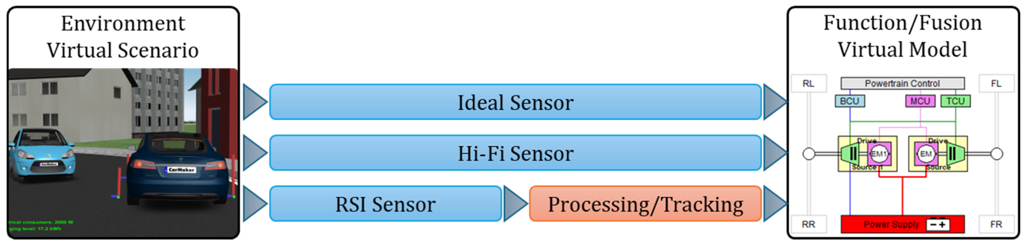
2.1. Virtual Sensor Model
- Camera sensors generate synthetic data on the recognition and classification of objects in the area [31,32,33], in addition to the vehicle’s positioning and orientation relative to close to objects and V2V (Vehicle-to-Vehicle) communication [34] based on the VLC (Visible Light Communication) principle [35]. The advantages of the camera sensor include the ability to provide data in real time, low latency in data acquisition and processing, adaptability to extreme lighting conditions (low lighting, bright lighting), accurate estimation of object position and orientation, and low production and implementation costs. The constraints of camera sensors include the need for a direct view of the surrounding objects, susceptibility to unexpected changes in lighting conditions, and the need for greater computer capacity due to the large quantities of data that are constantly generated.
- Radar sensor generates data based on the reflection duration of radio waves ToF (Time of Flight) when detecting nearby target vehicles [36,37] and uses ML methods to estimate the current and future positions of nearby vehicles [38], respectively, using DL (deep learning) methods to avoid collisions [39]. The benefits of radar sensors include the capacity to provide the location of target vehicles in real time, flexibility to severe weather conditions (rain, snow, fog), and low manufacturing and installation costs. The constraints of radar sensors include the requirement for increased computer capacity due to the massive volumes of data generated on a continuous basis, as well as a reliance on extra hardware systems and software.
- Lidar sensors provide a system based on generating a point cloud through 2D and 3D laser scanning for real-time localization of static and dynamic objects in proximity [40,41] and applies the YOLO (You Only Look Once) picture segmentation technique [42]. The advantages of lidar sensors include the ability to localize static and moving objects in proximity precisely. The disadvantages of lidar sensors include the need for greater computer power due to the large quantity of data generated continuously, sensitivity to bad weather conditions (rain, snow, fog), and high manufacturing and implementation costs.
- Sensor fidelity could be classified as high-, medium-, or low-income.
- Method for collecting information from the environment:
- (a)
- A deterministic strategy based on the simulation application’s mathematical apparatus and involving the usage of a vast volume of input parameters to represent the ideal behavior and response of the virtual sensor as accurately as possible;
- (b)
- A statistical technique based on statistical distribution functions, which include the normal, binomial, Poisson, or exponential distribution;
- (c)
- An electromagnetic field propagation approach to simulate electromagnetic wave propagation using Maxwell’s equations.
- The objective of using sensors is to develop a vehicle’s operating mode based on observed metrics and to perform diagnostics using AI-based maintenance techniques to define the smart maintenance regime.
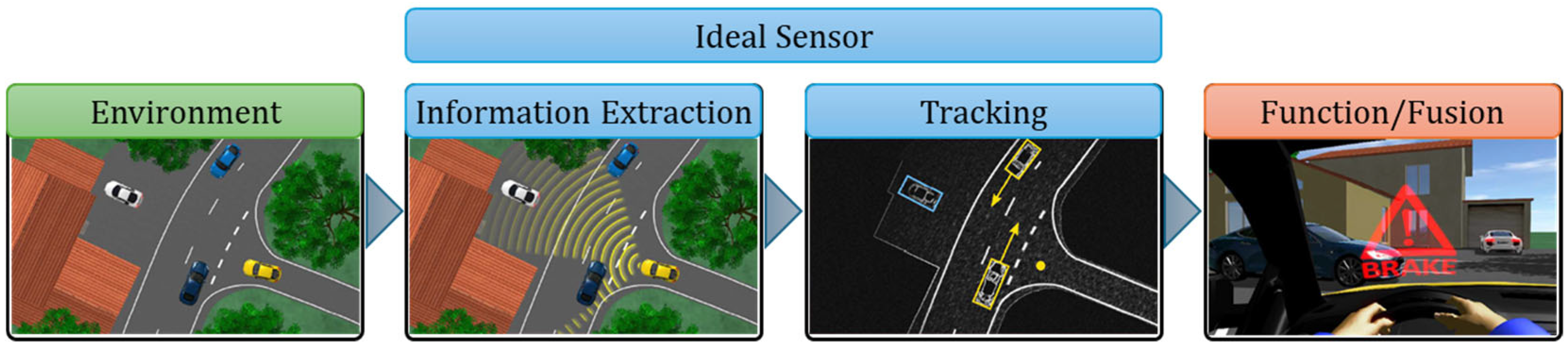
2.1.1. Ideal Sensors
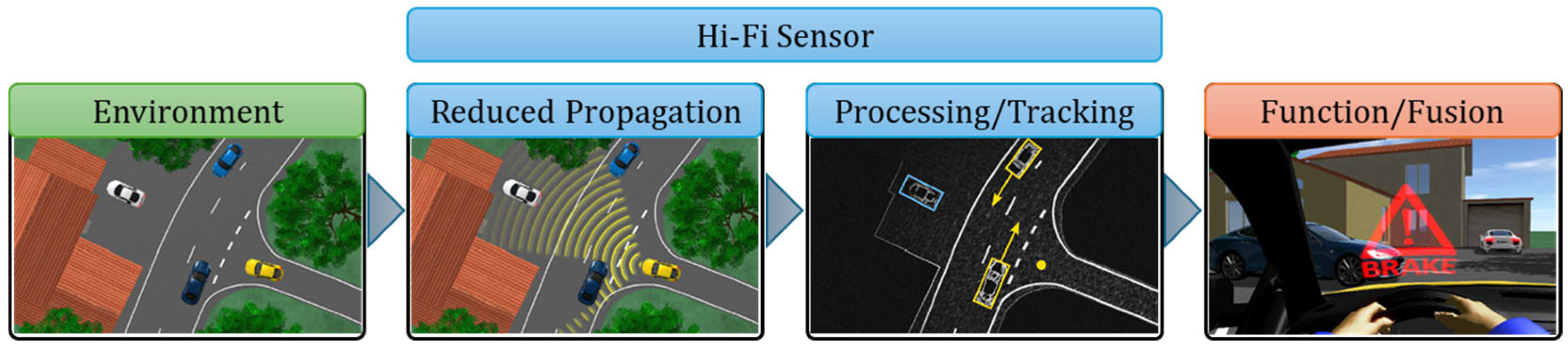
2.1.2. Hi-Fi Sensors
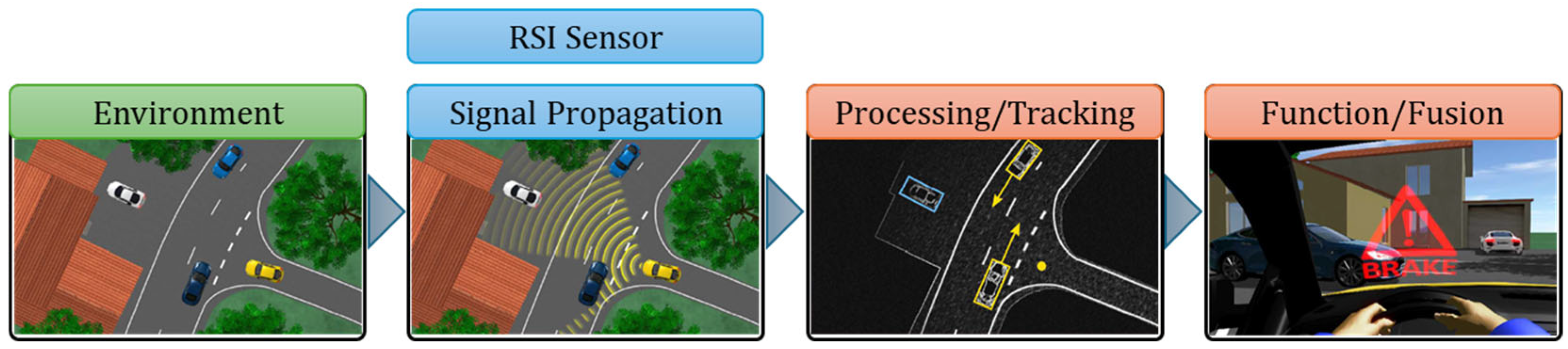
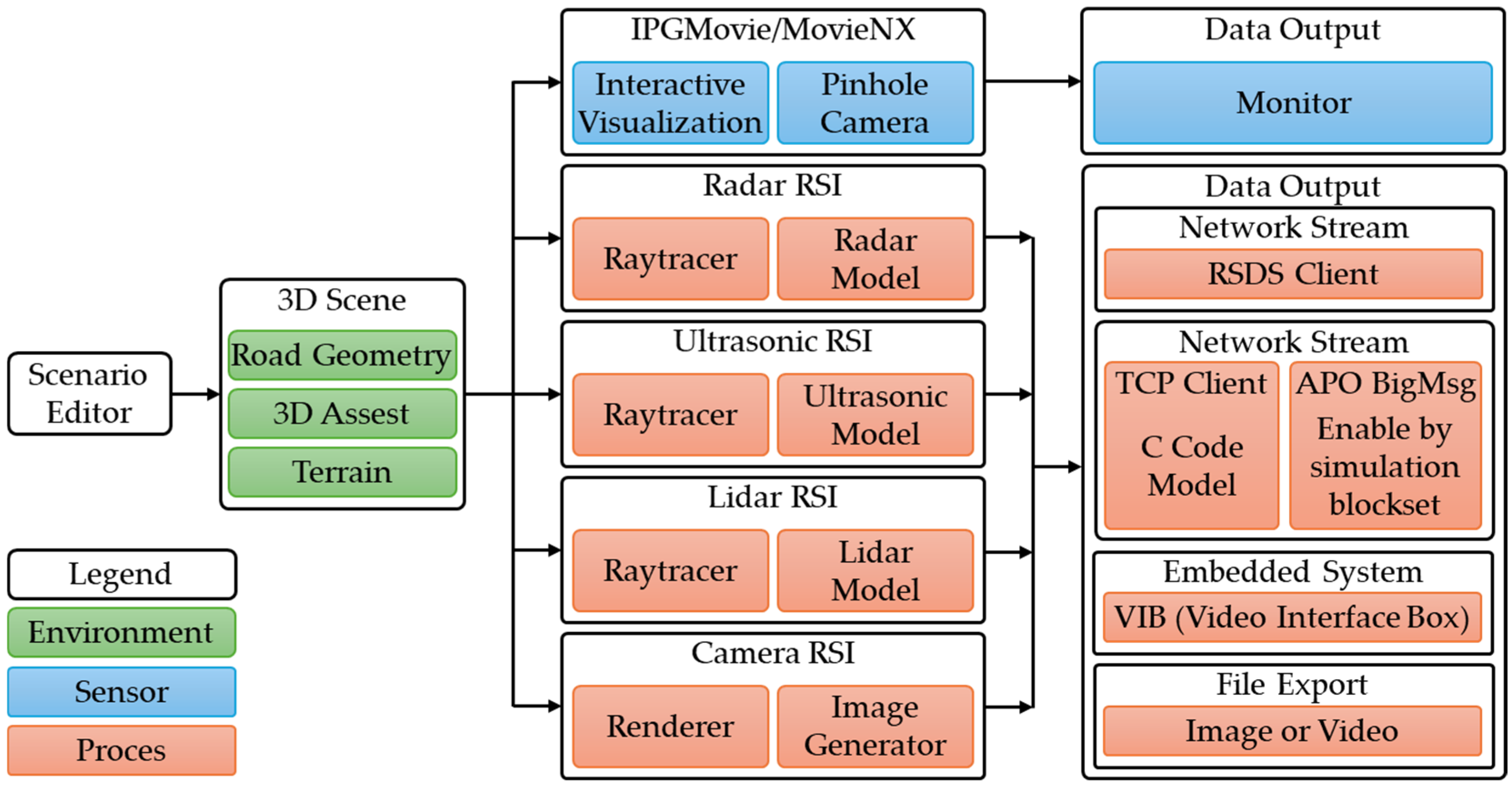
2.1.3. RSI Sensors
2.2. Virtual Vehicle and Environmental Model
3. Characteristics of the Virtual Sensor
3.1. Characteristics of Ideal Sensor
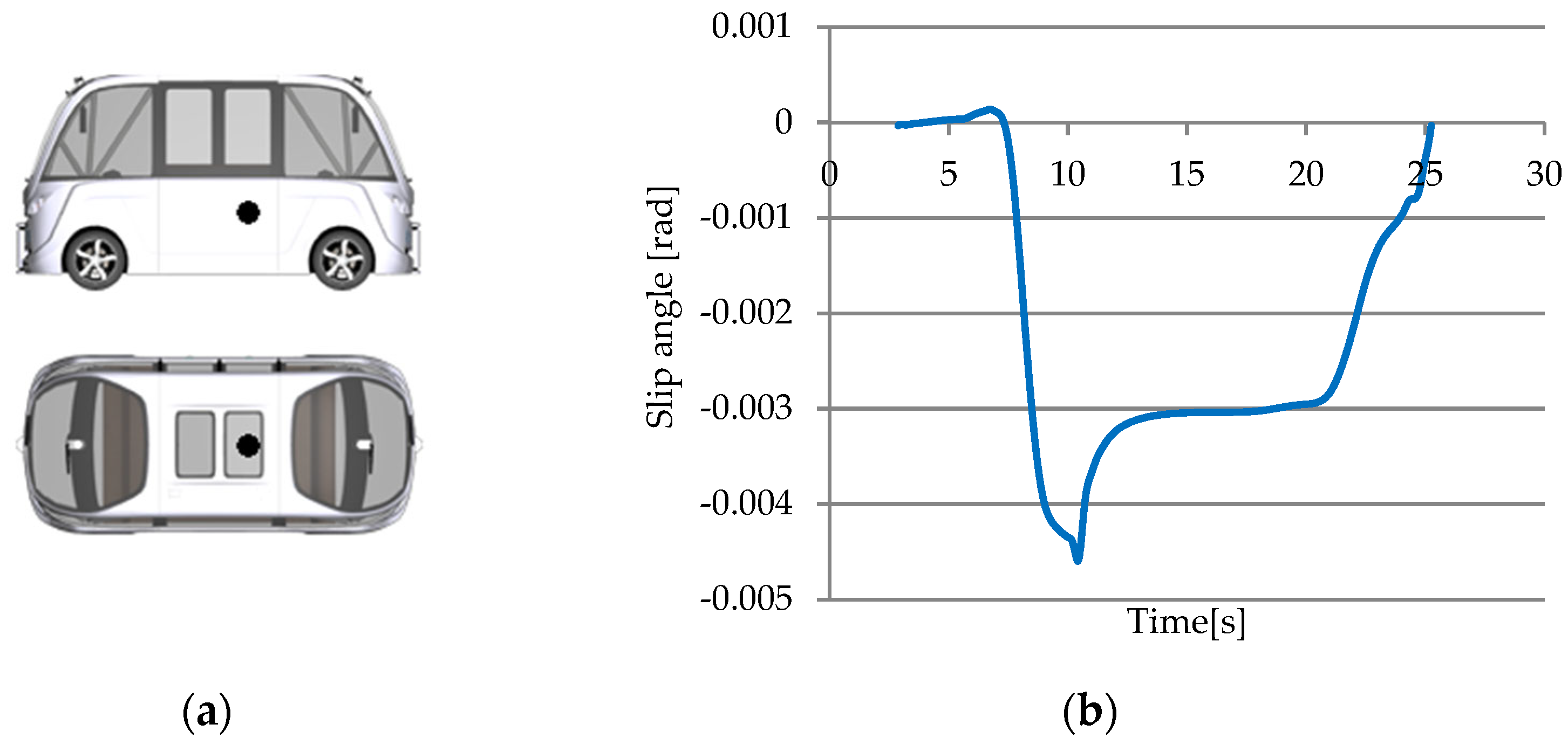
3.1.1. Slip Angle Sensor
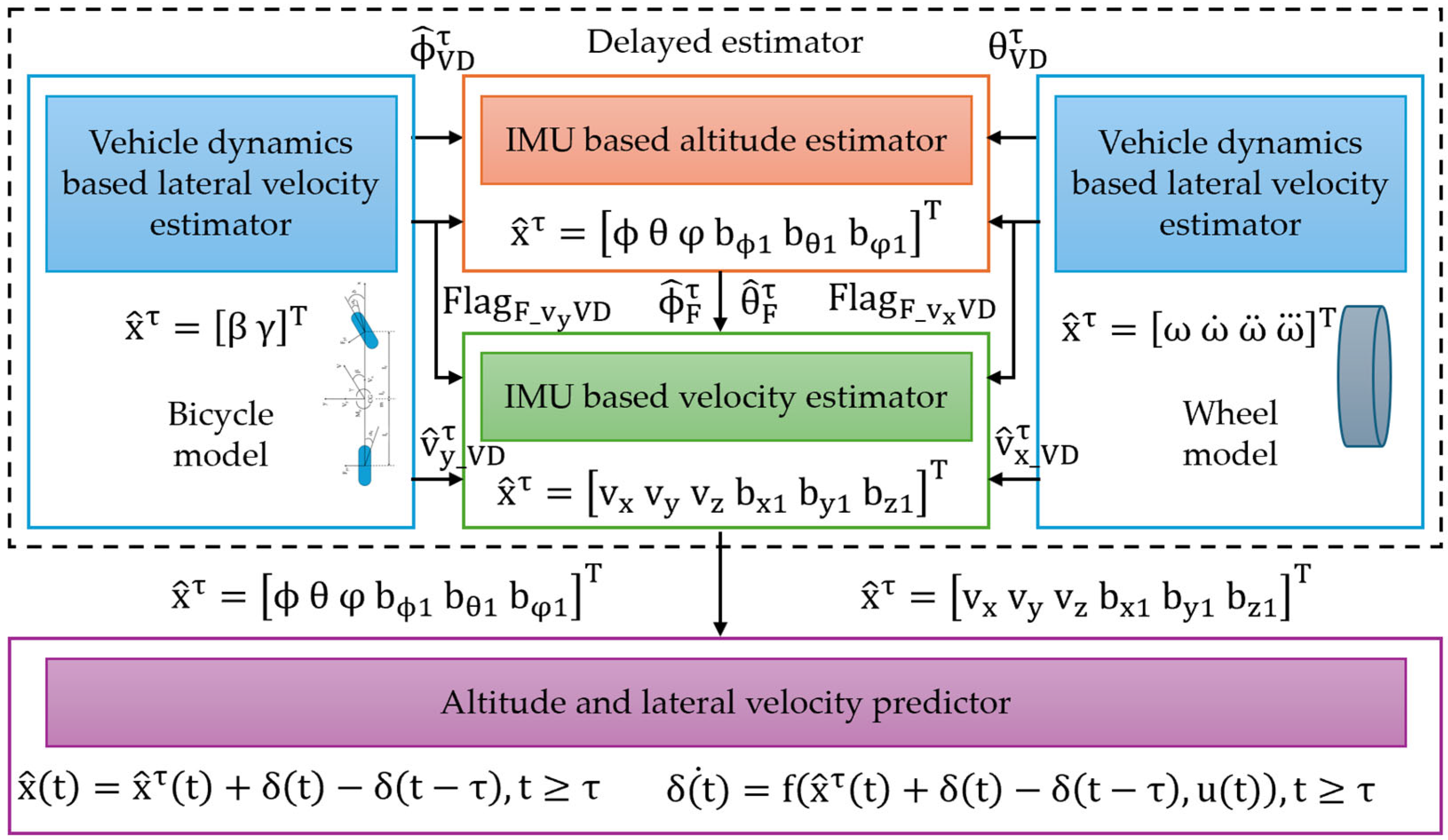
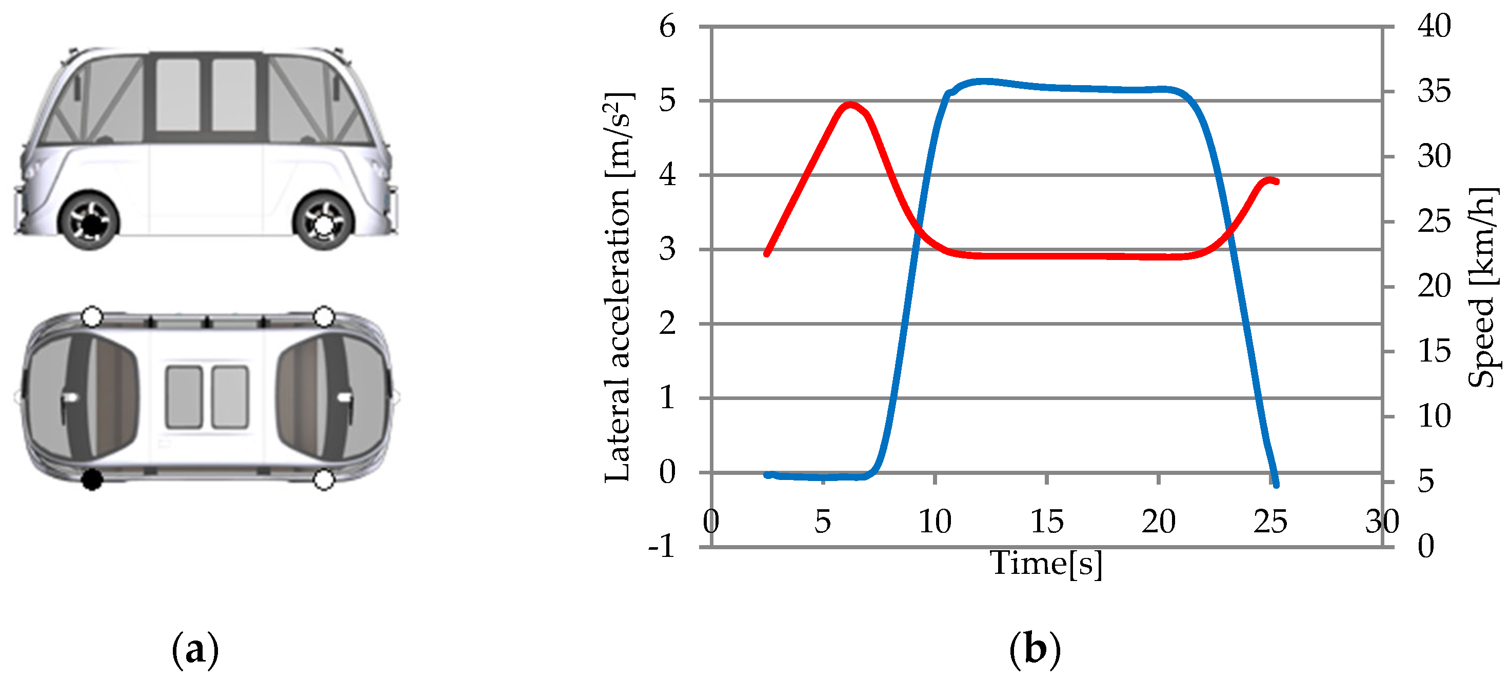
3.1.2. Inertial Sensor
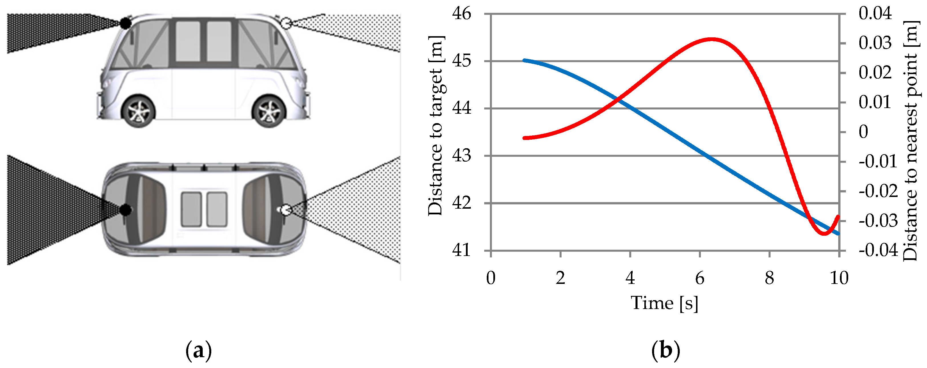
3.1.3. Object Sensor
- Nearest object—this is the closest visible object that is considered a relevant target;
- Nearest object in the path—this is the closest object within an interval of an estimated vehicle trajectory.
- Object ID, a name or a code used to identify an object;
- Path direction (reference and closest point);
- Relative distance and velocity (between the reference and the nearest positions);
- Relative orientation in the axle x-y-z (the reference point);
- Sensor frame’s x-y-z distances (between the reference and the nearest point);
- Sensor frame’s x-y-z velocity (between the reference and the nearest point);
- Flag object has been identified (in the sensor viewing area);
- Flag object has been identified (in the observation area);
- Incidence angles between the sensor beam and the object being detected from proximity;
- Width, height, length of the object, and height above the ground.
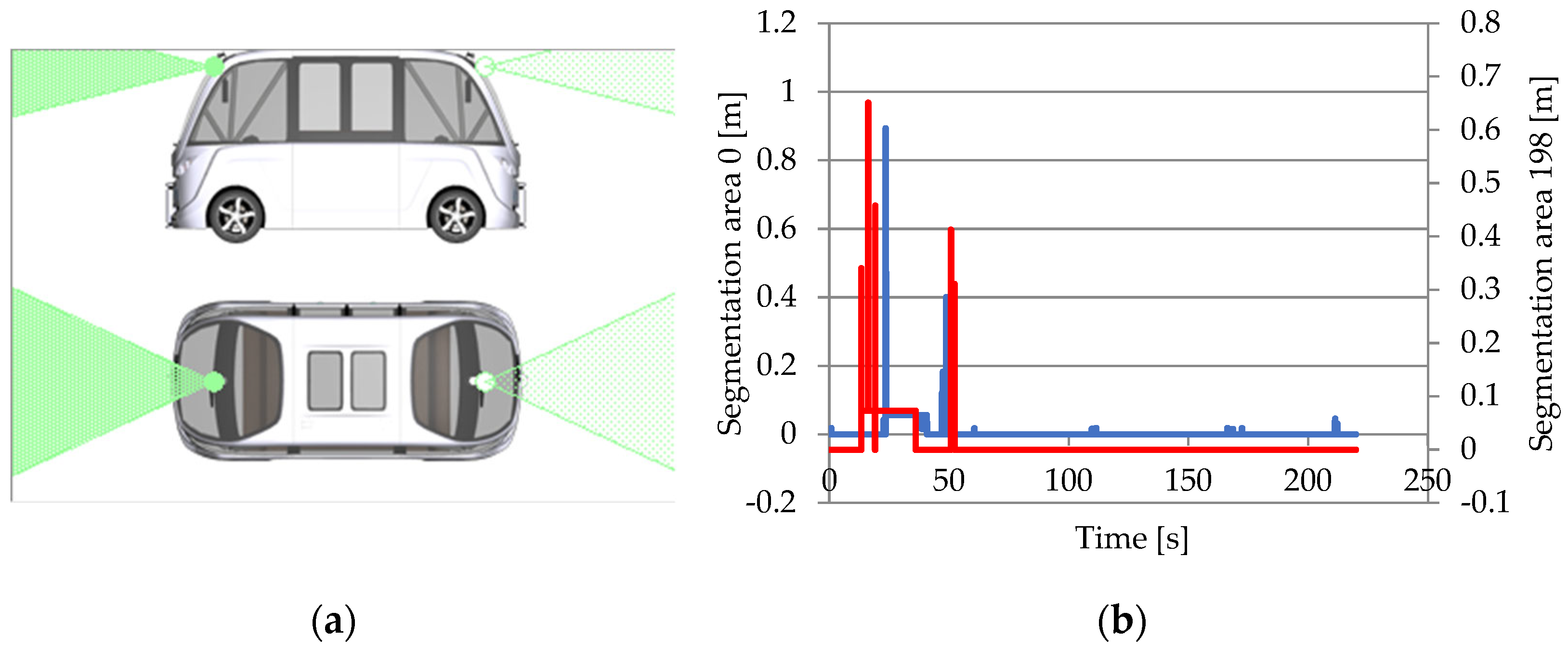
3.1.4. Free Space Sensor
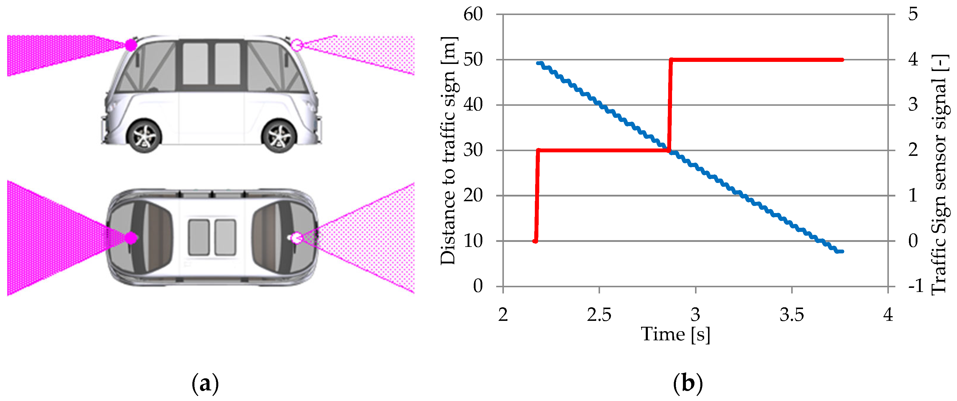
3.1.5. Traffic Sign Sensor
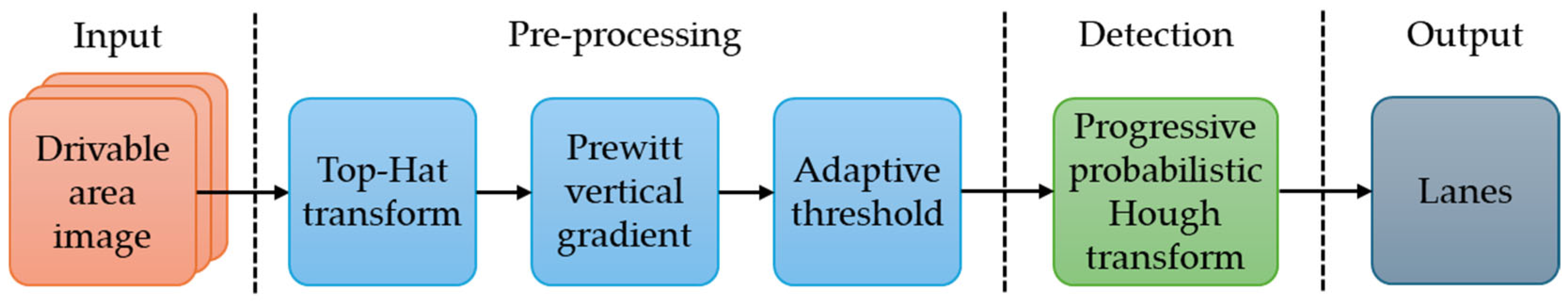
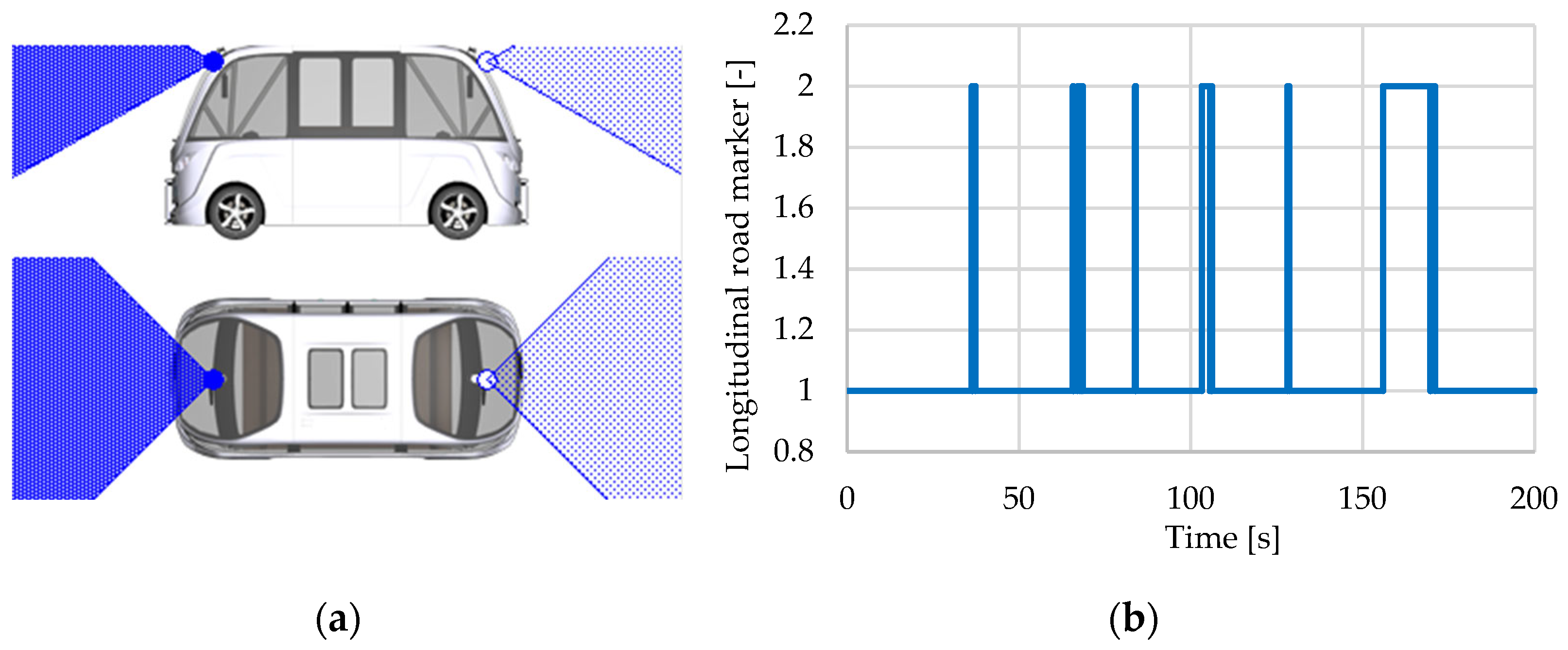
3.1.6. Line Sensor
3.1.7. Road Sensor
3.1.8. Object-by-Line Sensor
3.2. Characteristics of Hi-Fi Sensor
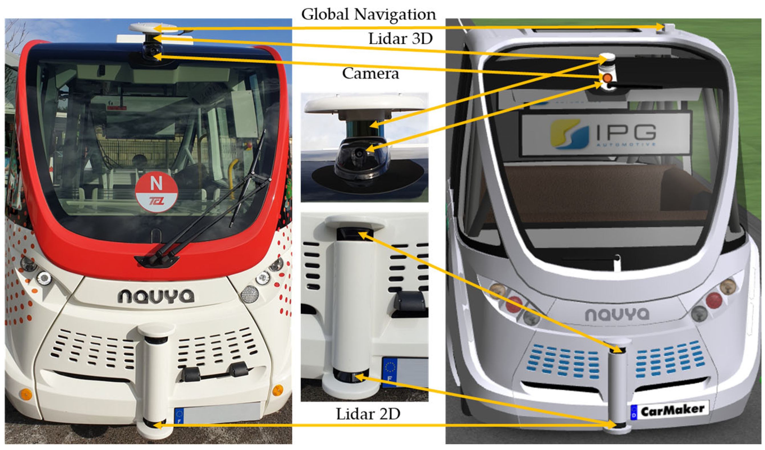
3.2.1. Camera Sensor
3.2.2. Global Navigation Sensor
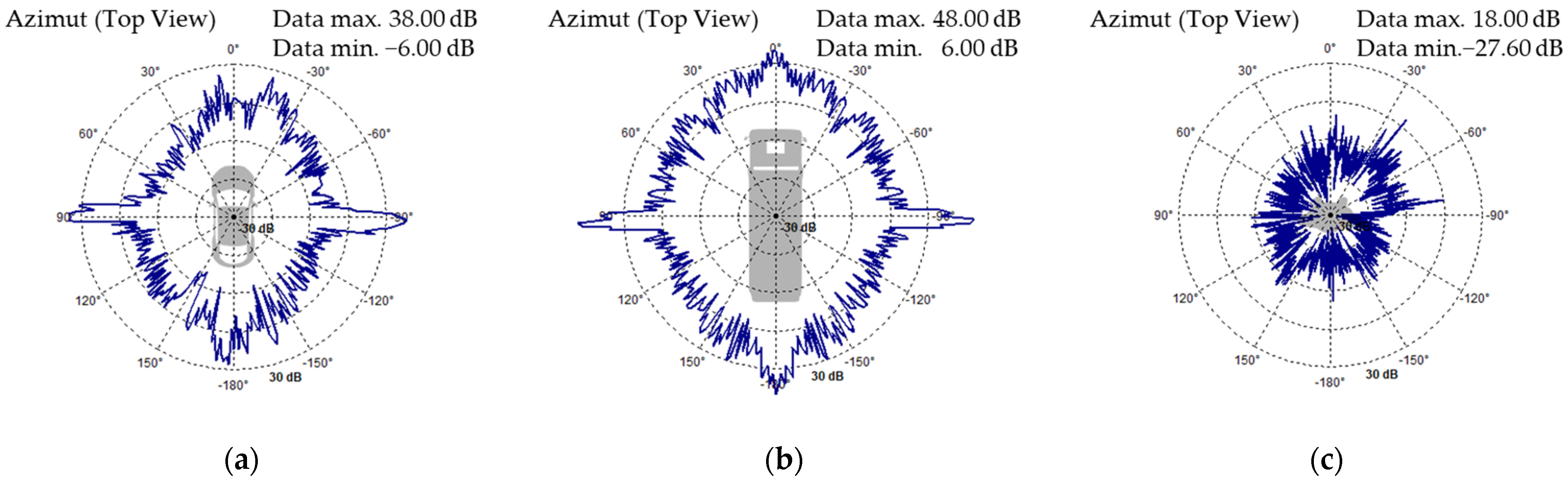
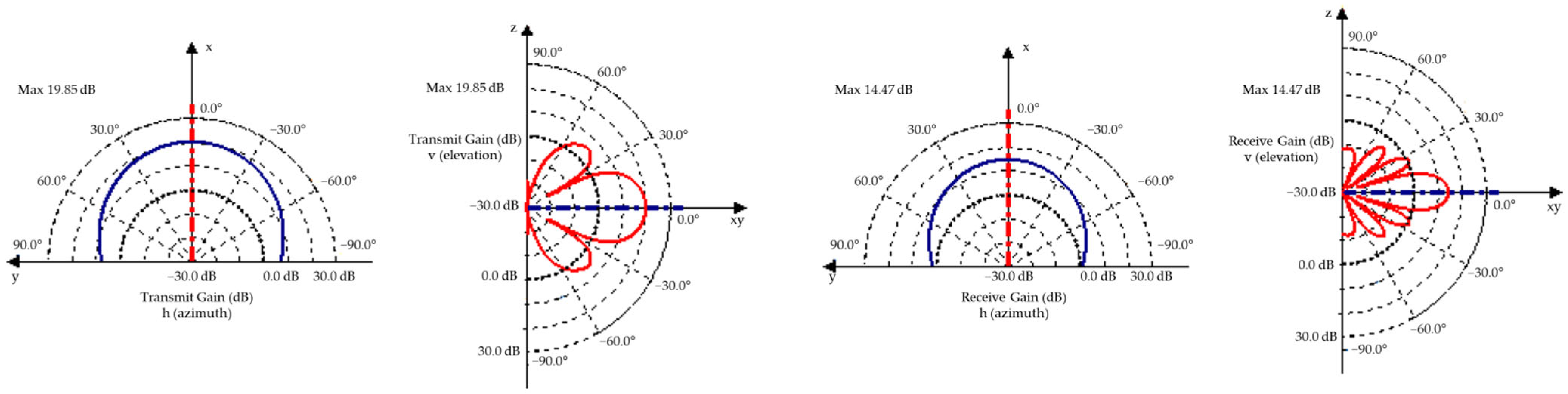
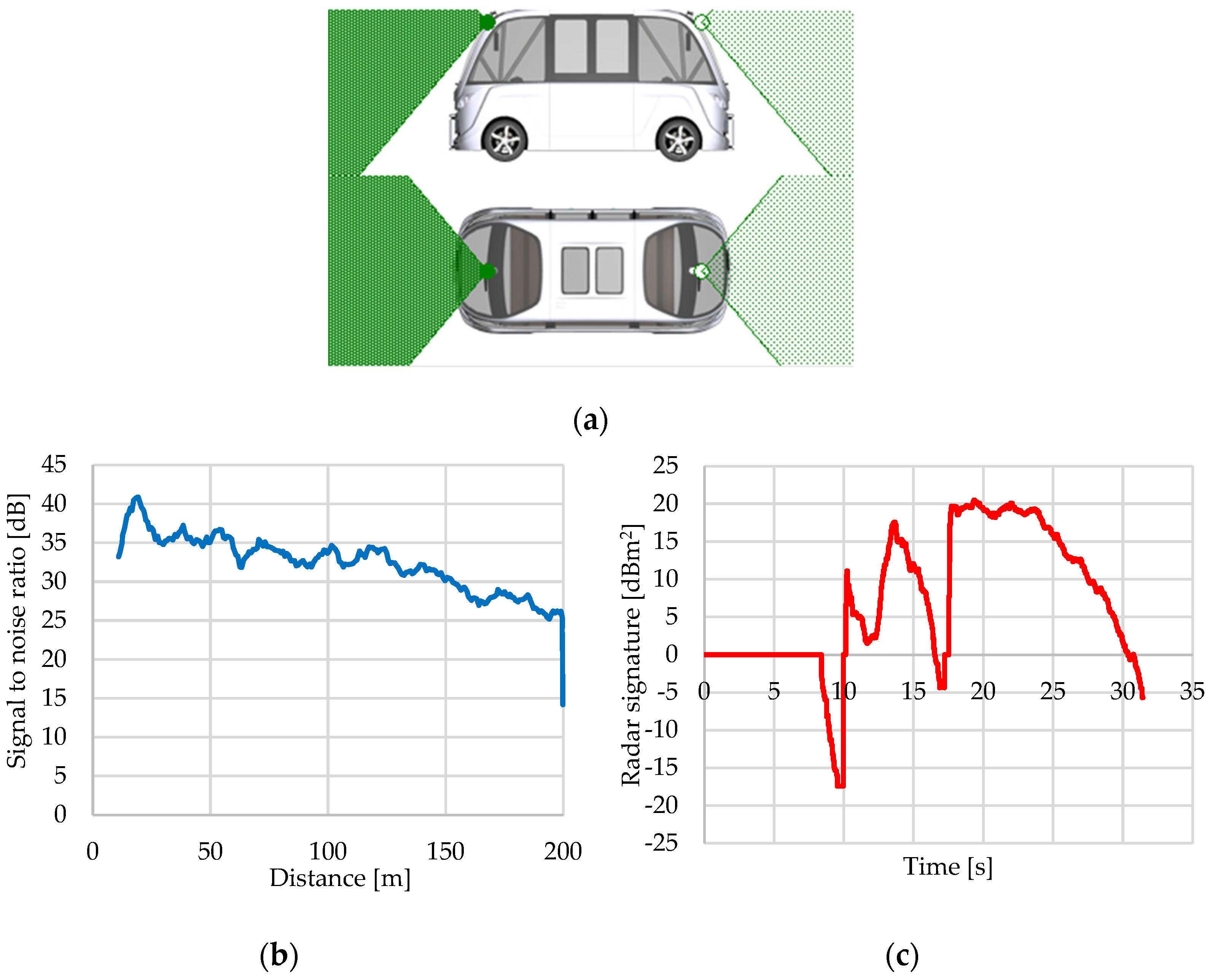
3.2.3. Radar Sensor
3.3. Characteristics of RSI Sensor
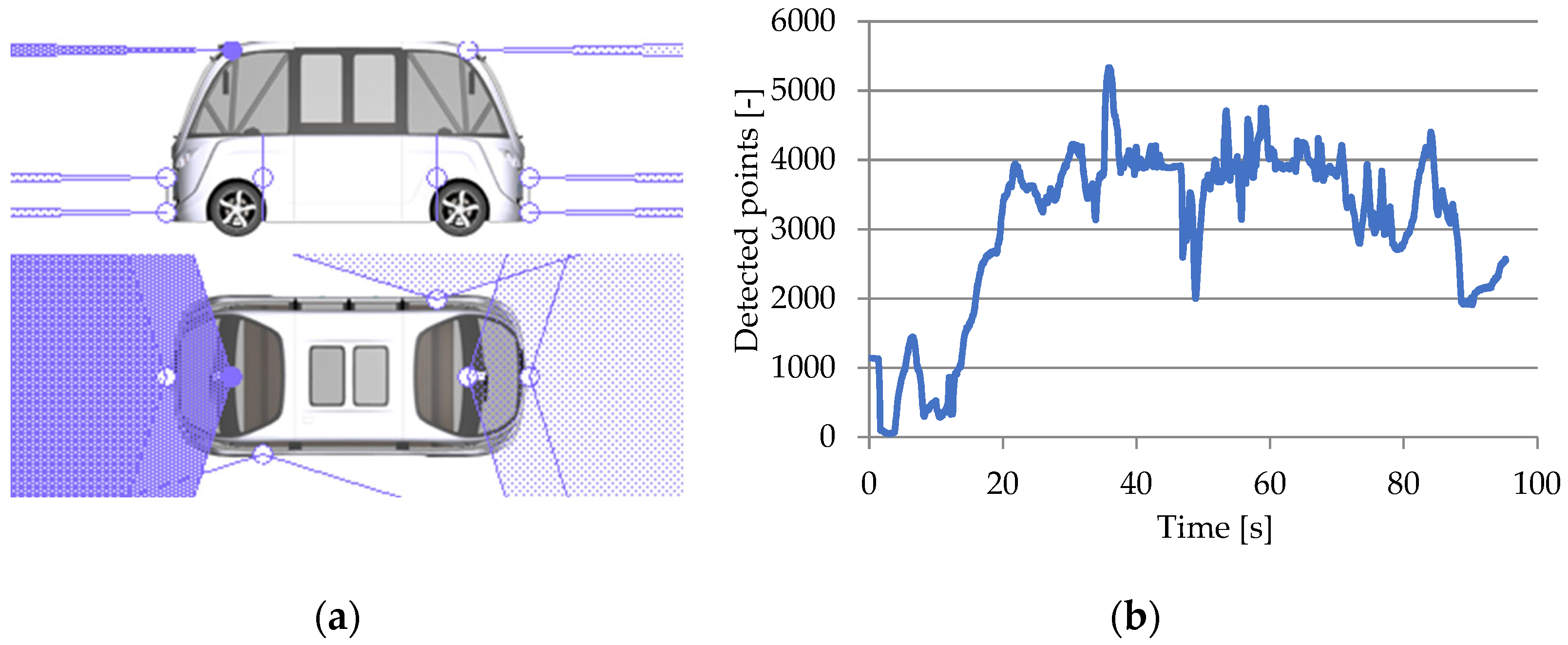
3.3.1. Lidar RSI Sensor
- Uniformly distributed diffuse reflected laser rays, regardless of the direction of the incident ray (Lambertian reflection), with the intensity of the reflected ray decreased by the inverse of the angle between the incident ray and the normal of the reflective surface;
- Retroreflective, meaning that incident laser rays are reflected back in the direction of the emitter, with the intensity of the reflected ray being reduced based on the reflectance parameters and incident angle;
- Specular, meaning that the incident and reflected laser rays form identical angles with the normal of the reflective surface, and the incident and reflected laser rays are in the identical plane;
- Transmissive, meaning that the incident laser photons keep their course but are attenuated by transmission.
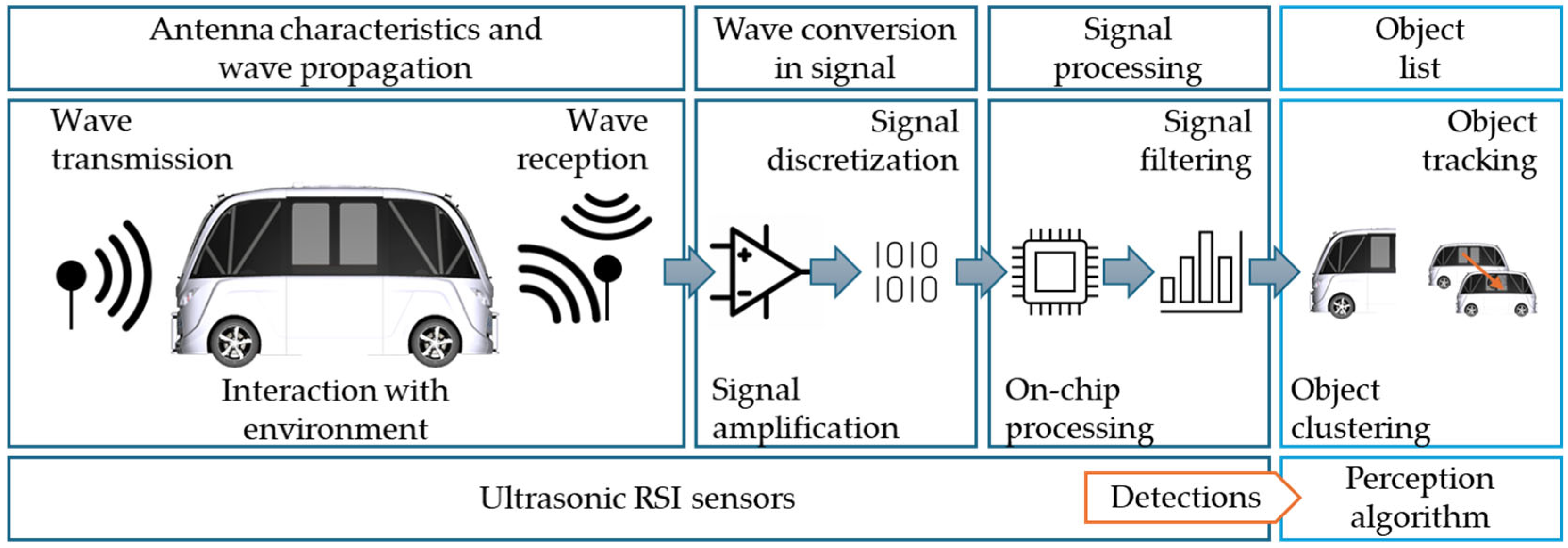
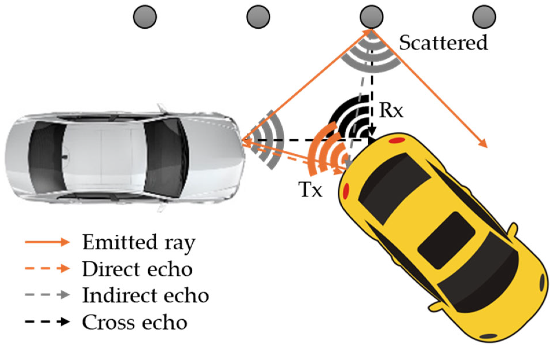
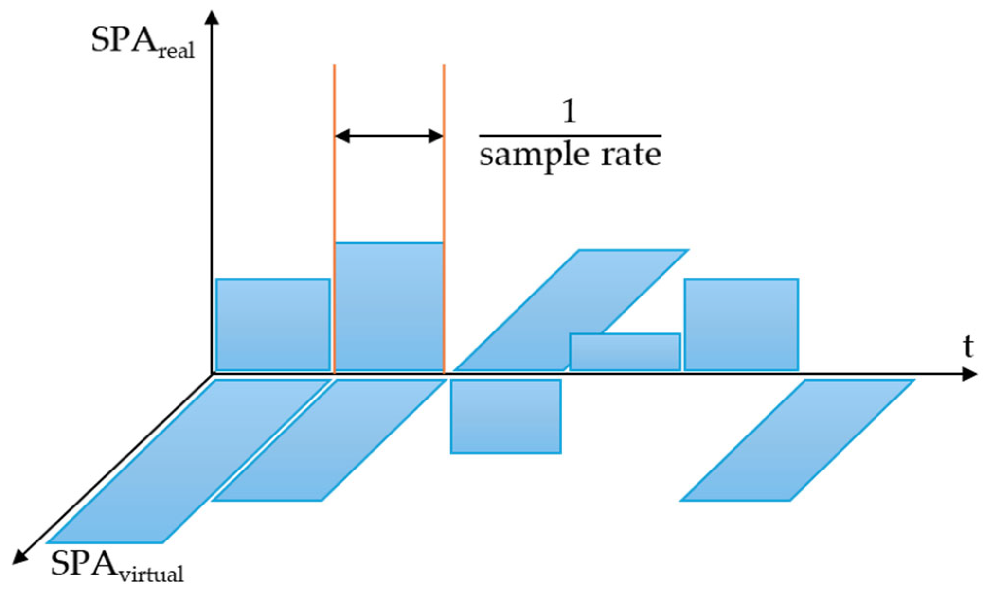
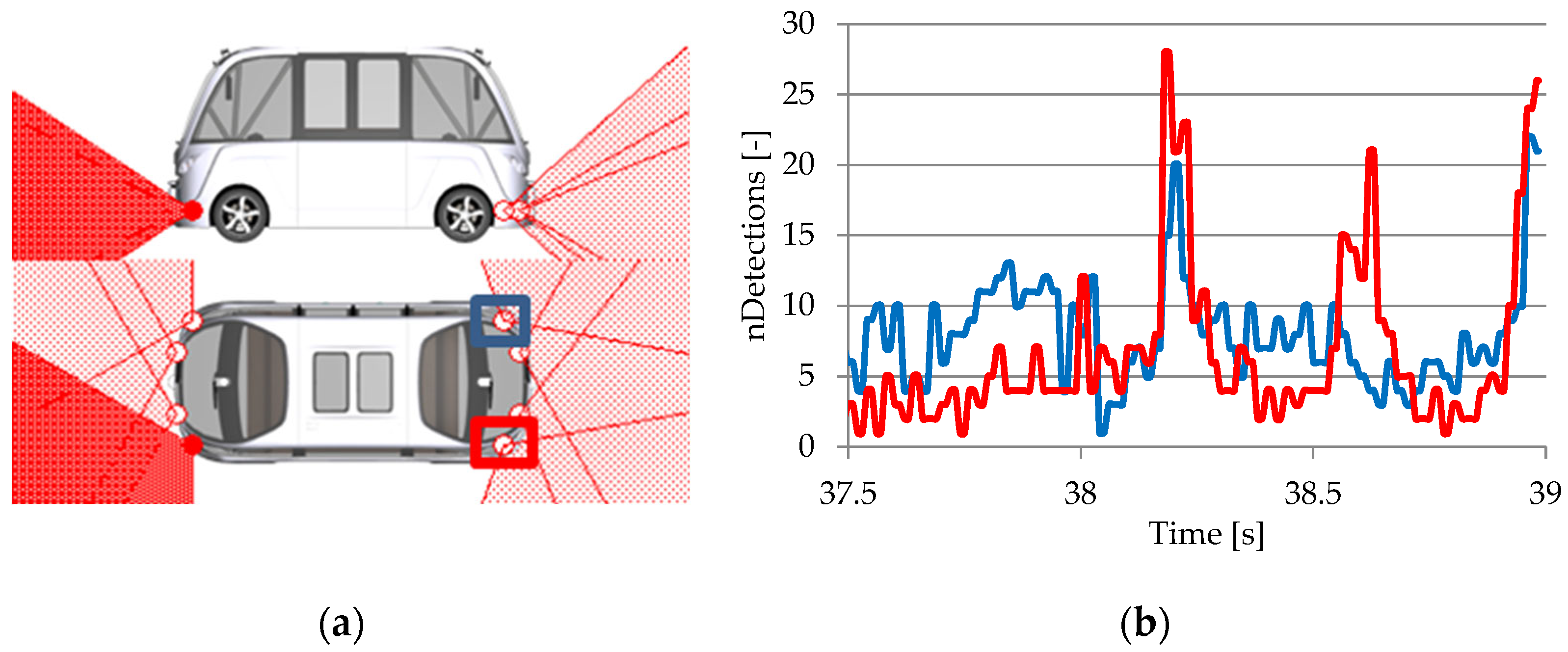
3.3.2. Ultrasonic RSI Sensor
- Direct Echo: The acoustic pressure wave is reflected once by an object in close proximity and received by the emitting sensor.
- Indirect Echo: The acoustic pressure wave is reflected at least twice by objects or surfaces in the vicinity and received by the emitting sensor.
- Repeated Echo: The emitting sensor receives the acoustic pressure wave after it has been reflected by nearby objects or surfaces.
- Cross Echo: The reflected acoustic pressure wave is received by a sensor other than the originating sensor, resulting in a propagation mode known as cross echo.
- Road Clutter: This occurs when the acoustic pressure wave is reflected by bumps or irregularities in the roadway.
4. Virtual Sensor Parametrization
4.1. Ideal Sensor Parametrization
4.2. Hi-Fi Sensor Parametrization
4.3. RSI Sensor Parametrization
5. Discussion
6. Conclusions
- Cost-effectiveness—virtual sensors are affordable alternatives to real sensors.
- Reduced vehicle mass—replacing physical sensors and associated wiring and connectors helps to reduce vehicle weight, leading to fuel and energy savings and lower emissions.
- Software-based—virtual sensors are developed using software applications and do not require additional hardware.
- Remote updates—firmware upgrades can be performed remotely via the Over-The-Air method, eliminating the need for physical interventions.
- Improved data accuracy and resolution—virtual sensors can improve data accuracy and resolution by merging information from multiple sources and by using data fusion algorithms.
- Expanded coverage—they can provide coverage to locations where physical sensors are unavailable.
- Preprocessing and optimization—when integrated into an embedded system, they can preprocess data, and perform error correction, merging, and optimization of input data.
- Flexibility—they can be simple or sophisticated, depending on the simulated activities and their consequences.
- Data accessibility—they can increase data accessibility from physical sensors, facilitating collaboration and efficient use of resources in interconnected systems like IoT.
- Reduced testing costs and time—using virtual sensors, developers can significantly reduce the cost and time associated with physical testing.
- Exploration of a wider range of scenarios—virtual sensors allow for exploring a wider range of scenarios and edge cases.
Author Contributions
Funding
Institutional Review Board Statement
Informed Consent Statement
Data Availability Statement
Acknowledgments
Conflicts of Interest
Abbreviations
| ABS | Antilock Braking System |
| ADAS | Advanced Driver Assistance System |
| ACC | Adaptive Cruise Control |
| AD | Autonomous driving |
| AEB | Automatic Emergency Braking |
| AI | Artificial Intelligence |
| AWD | All-Wheel Drive |
| BiSeNet | Bilateral Segmentation Network |
| CNN | Convolutional neural network |
| D-GNSS | Differential-Global Navigation Satellite System |
| CPU | Central Processing Unit |
| DL | Deep Learning |
| DMS | Driver Monitoring System |
| DPM | Deformable Part Model |
| DTw | Digital Twin |
| DVM | Double Validation Metric |
| EBA | Emergency Brake Assist |
| ECEF | Earth-Centered, Earth-Fixed |
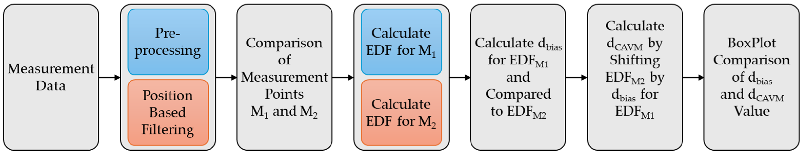
| EDF | Empirical Cumulative Distribution Function |
| EM | Energy Management |
| ESC | Electronic Stability Control |
| FC | Fuel Consumption |
| FCW | Forward Collision Warning |
| FET | Field-Effect Transistor |
| FoV | Field-Of-View |
| GCS | Geographic Coordinate System |
| GDOP | Geometric Dilution of Precision |
| GNN | Global Nearest Neighbor |
| GNSS | Global Navigation Satellite System |
| GPS | Global Positioning System |
| GPU | Graphics Processing Unit |
| HD | High-Definition |
| Hi-Fi | High fidelity |
| HiL | Hardware-in-the-Loop |
| HV | High voltage |
| ID | Identifier |
| ILA | Intelligent Light Assist |
| IMU | Inertial Measurement Unit |
| IoT | Internet of Things |
| LDW | Lane Departure Warning |
| Lidar | Light detection and ranging |
| LK | Lane Keeping |
| LKA | Lane Keeping Assist |
| LV | Low voltage |
| MEMS | Micro-Electro-Mechanical Systems |
| ML | Machine Learning |
| MMS | Mobile Mapping System |
| OTA | Over-The-Air |
| PA | Park Assist |
| PPHT | Progressive Probabilistic Hough Transform |
| POI | Point Of Interest |
| PS | Physical sensors |
| PT | Powertrain |
| QTC | Quantum Tunneling Composite |
| RCS | Radar Cross-Section |
| RSI | Raw Signal Interface |
| RTK | Real-Time Kinematic |
| SAS | Smart Airbag System |
| SD | Sign Detection |
| SiL | Software-in-the-Loop |
| SLAM | Simultaneous localization And mapping |
| SNR | Signal-to-noise ratio |
| SPA | Sound Pressure Amplitude |
| SRTM | Shuttle Radar Topography Mission |
| ToF | Time of Flight |
| TSA | Traffic Sign Assist |
| V2I | Vehicle-to-Infrastructure |
| V2V | Vehicle-to-Vehicle |
| VDM | Vehicle dynamics model |
| VLC | Visible Light Communication |
| VS | Virtual sensors |
| WLD | Wheel Lifting Detection |
| YOLO | You Only Look Once |
References
- Martin, D.; Kühl, N.; Satzger, G. Virtual Sensors. Bus. Inf. Syst. Eng. 2021, 63, 315–323. [Google Scholar] [CrossRef]
- Dahiya, R.; Ozioko, O.; Cheng, G. Sensory Systems for Robotic Applications; MIT Press: Cambridge, MA, USA, 2022. [Google Scholar] [CrossRef]
- Šabanovič, E.; Kojis, P.; Šukevičius, Š.; Shyrokau, B.; Ivanov, V.; Dhaens, M.; Skrickij, V. Feasibility of a Neural Network-Based Virtual Sensor for Vehicle Unsprung Mass Relative Velocity Estimation. Sensors 2021, 21, 7139. [Google Scholar] [CrossRef] [PubMed]
- Persson, J.A.; Bugeja, J.; Davidsson, P.; Holmberg, J.; Kebande, V.R.; Mihailescu, R.-C.; Sarkheyli-Hägele, A.; Tegen, A. The Concept of Interactive Dynamic Intelligent Virtual Sensors (IDIVS): Bridging the Gap between Sensors, Services, and Users through Machine Learning. Appl. Sci. 2023, 13, 6516. [Google Scholar] [CrossRef]
- Ambarish, P.; Mitradip, B.; Ravinder, D. Solid-State Sensors; IEEE Press Series on Sensors; Wiley-IEEE Press: Hoboken, NJ, USA, 2023. [Google Scholar] [CrossRef]
- Shin, H.; Kwak, Y. Enhancing digital twin efficiency in indoor environments: Virtual sensor-driven optimization of physical sensor combinations. Automat. Constr. 2024, 161, 105326. [Google Scholar] [CrossRef]
- Stanley, M.; Lee, J. Sensor Analysis for the Internet of Things; Morgan & Claypool Publishers: San Rafael, CA, USA; Arizona State University: Tempe, AZ, USA, 2018. [Google Scholar]
- Stetter, R. A Fuzzy Virtual Actuator for Automated Guided Vehicles. Sensors 2020, 20, 4154. [Google Scholar] [CrossRef]
- Xie, J.; Yang, R.; Gooi, H.B.; Nguyen, H. PID-based CNN-LSTM for accuracy-boosted virtual sensor in battery thermal management system. Appl. Energ. 2023, 331, 120424. [Google Scholar] [CrossRef]
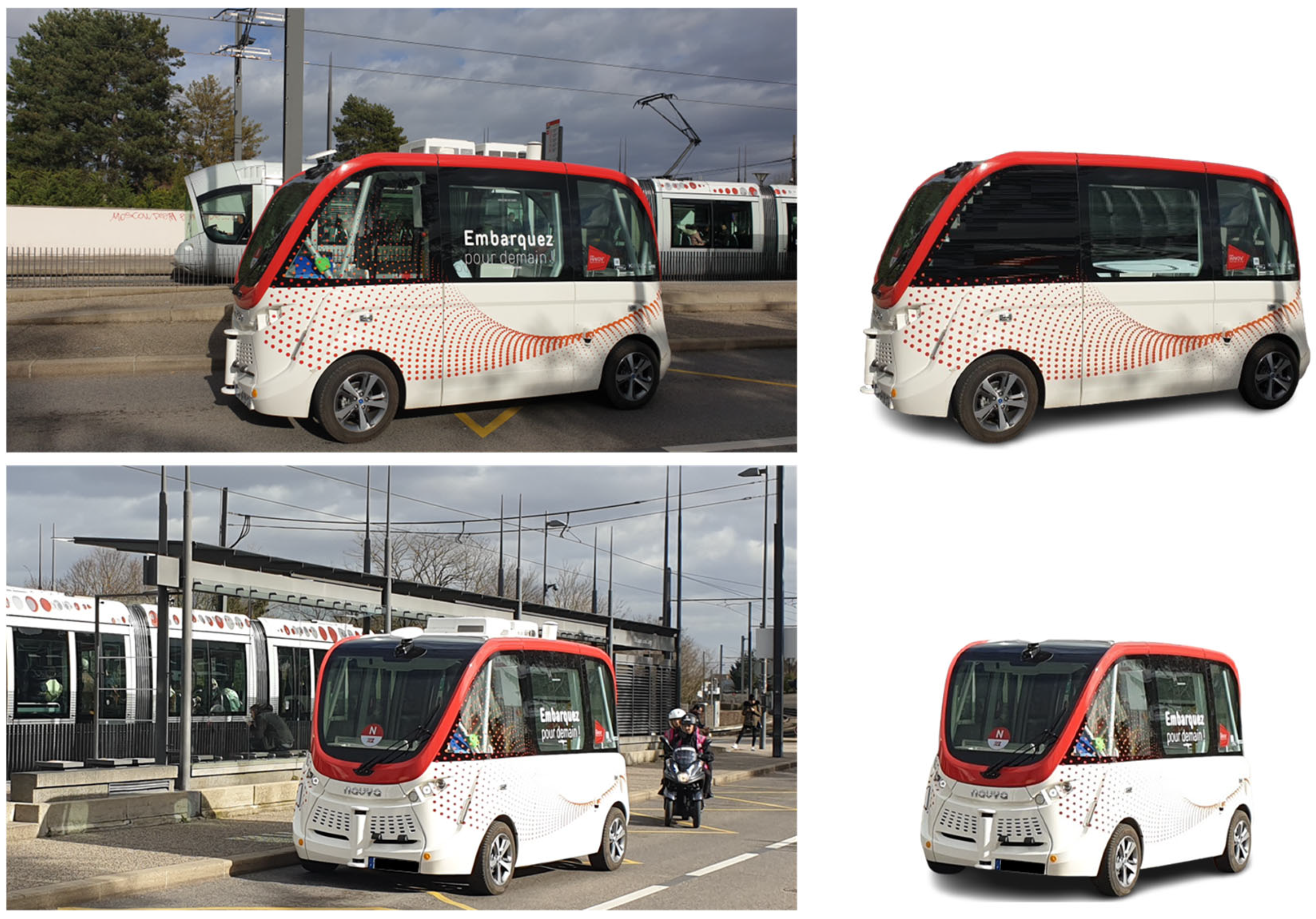
- Iclodean, C.; Cordos, N.; Varga, B.O. Autonomous Shuttle Bus for Public Transportation: A Review. Energies 2020, 13, 2917. [Google Scholar] [CrossRef]
- Fabiocchi, D.; Giulietti, N.; Carnevale, M.; Giberti, H. AI-Driven Virtual Sensors for Real-Time Dynamic Analysis of Me-chanisms: A Feasibility Study. Machines 2024, 12, 257. [Google Scholar] [CrossRef]
- Kabadayi, S.; Pridgen, A.; Julien, C. Virtual sensors: Abstracting data from physical sensors. In Proceedings of the IEEE International Symposium on a World of Wireless, Mobile and Multimedia Networks, Buffalo-Niagara Falls, NY, USA, 26–29 June 2006. [Google Scholar] [CrossRef]
- Compredict. Available online: https://compredict.ai/virtual-sensors-replacing-vehicle-hardware-sensors/ (accessed on 6 February 2025).
- Prokhorov, D. Virtual Sensors and Their Automotive Applications. In Proceedings of the 2005 International Conference on Intelligent Sensors, Sensor Networks and Information Processing, Melbourne, VIC, Australia, 5–8 December 2005. [Google Scholar] [CrossRef]
- Forssell, U.; Ahlqvist, S.; Persson, N.; Gustafsson, F. Virtual Sensors for Vehicle Dynamics Applications. In Advanced Microsystems for Automotive Applications 2001; VDI-Buch; Krueger, S., Gessner, W., Eds.; Springer: Berlin/Heidelberg, Germany, 2012. [Google Scholar] [CrossRef]
- Hu, X.H.; Cao, L.; Luo, Y.; Chen, A.; Zhang, E.; Zhang, W. A Novel Methodology for Comprehensive Modeling of the Kinetic Behavior of Steerable Catheters. IEEE/ASME Trans. Mechatron. 2019, 24, 1785–1797. [Google Scholar] [CrossRef]
- Cummins. Available online: https://www.cummins.com/news/2024/03/18/virtual-sensors-and-their-role-energy-future (accessed on 6 February 2025).
- Bucaioni, A.; Pelliccione, P.; Mubeen, S. Modelling centralised automotive E/E software architectures. Adv. Eng. Inform. 2024, 59, 102289. [Google Scholar] [CrossRef]
- Zhang, Q.; Shen, S.; Li, H.; Cao, W.; Tang, W.; Jiang, J.; Deng, M.; Zhang, Y.; Gu, B.; Wu, K.; et al. Digital twin-driven intelligent production line for automotive MEMS pressure sensors. Adv. Eng. Inform. 2022, 54, 101779. [Google Scholar] [CrossRef]
- Ida, N. Sensors, Actuators, and Their Interfaces: A multidisciplinary Introduction, 2nd ed.; The Institution of Engineering and Technology: London, UK, 2020. [Google Scholar] [CrossRef]
- Masti, D.; Bernardini, D.; Bemporad, A. A machine-learning approach to synthesize virtual sensors for parameter-varying systems. Eur. J. Control. 2021, 61, 40–49. [Google Scholar] [CrossRef]
- Paepae, T.; Bokoro, P.N.; Kyamakya, K. From fully physical to virtual sensing for water quality assessment: A comprehensive review of the relevant state-of-the-art. Sensors 2021, 21, 6971. [Google Scholar] [CrossRef] [PubMed]
- Tihanyi, V.; Tettamanti, T.; Csonthó, M.; Eichberger, A.; Ficzere, D.; Gangel, K.; Hörmann, L.B.; Klaffenböck, M.A.; Knauder, C.; Luley, P.; et al. Motorway Measurement Campaign to Support R&D Activities in the Field of Automated Driving Technologies. Sensors 2021, 21, 2169. [Google Scholar] [CrossRef]
- Tactile Mobility. Available online: https://tactilemobility.com/ (accessed on 6 February 2025).
- Compredict-Virtual Sensor Platform. Available online: https://compredict.ai/virtual-sensor-platform/ (accessed on 6 February 2025).
- Mordor Intellingence. Available online: https://www.mordorintelligence.com/industry-reports/virtual-sensors-market (accessed on 6 February 2025).
- Iclodean, C.; Varga, B.O.; Cordoș, N. Autonomous Driving Technical Characteristics. In Autonomous Vehicles for Public Transportation, Green Energy and Technology; Springer: Berlin/Heidelberg, Germany, 2022; pp. 15–68. [Google Scholar] [CrossRef]
- SAE. Available online: https://www.sae.org/standards/content/j3016_202104/ (accessed on 6 February 2025).
- Muhovič, J.; Perš, J. Correcting Decalibration of Stereo Cameras in Self-Driving Vehicles. Sensors 2020, 20, 3241. [Google Scholar] [CrossRef] [PubMed]
- Hamidaoui, M.; Talhaoui, M.Z.; Li, M.; Midoun, M.A.; Haouassi, S.; Mekkaoui, D.E.; Smaili, A.; Cherraf, A.; Benyoub, F.Z. Survey of Autonomous Vehicles’ Collision Avoidance Algorithms. Sensors 2025, 25, 395. [Google Scholar] [CrossRef]
- Cabon, Y.; Murray, N.; Humenberger, M. Virtual KITTI 2. arXiv 2020, arXiv:2001.10773. [Google Scholar] [CrossRef]
- Mallik, A.; Gaopande, M.L.; Singh, G.; Ravindran, A.; Iqbal, Z.; Chao, S.; Revalla, H.; Nagasamy, V. Real-time Detection and Avoidance of Obstacles in the Path of Autonomous Vehicles Using Monocular RGB Camera. SAE Int. J. Adv. Curr. Pract. Mobil. 2022, 5, 622–632. [Google Scholar] [CrossRef]
- Zhe, T.; Huang, L.; Wu, Q.; Zhang, J.; Pei, C.; Li, L. Inter-Vehicle Distance Estimation Method Based on Monocular Vision Using 3D Detection. IEEE Trans. Veh. Technol. 2020, 69, 4907–4919. [Google Scholar] [CrossRef]
- Rill, R.A.; Faragó, K.B. Collision avoidance using deep learning-based monocular vision. SN Comput. Sci. 2021, 2, 375. [Google Scholar] [CrossRef]
- He, J.; Tang, K.; He, J.; Shi, J. Effective vehicle-to-vehicle positioning method using monocular camera based on VLC. Opt. Express 2020, 28, 4433–4443. [Google Scholar] [CrossRef] [PubMed]
- Choi, W.Y.; Yang, J.H.; Chung, C.C. Data-Driven Object Vehicle Estimation by Radar Accuracy Modeling with Weighted Interpolation. Sensors 2021, 21, 2317. [Google Scholar] [CrossRef] [PubMed]
- Muckenhuber, S.; Museljic, E.; Stettinger, G. Performance evaluation of a state-of-the-art automotive radar and corres-ponding modeling approaches based on a large labeled dataset. J. Intell. Transport. Syst. 2022, 26, 655–674. [Google Scholar] [CrossRef]
- Sohail, M.; Khan, A.U.; Sandhu, M.; Shoukat, I.A.; Jafri, M.; Shin, H. Radar sensor based Machine Learning approach for precise vehicle position estimation. Sci. Rep. 2023, 13, 13837. [Google Scholar] [CrossRef]
- Srivastav, A.; Mandal, S. Radars for autonomous driving: A review of deep learning methods and challenges. IEEE Access 2023, 11, 97147–97168. [Google Scholar] [CrossRef]
- Poulose, A.; Baek, M.; Han, D.S. Point cloud map generation and localization for autonomous vehicles using 3D lidar scans. In Proceedings of the 2022 27th Asia Pacific Conference on Communications (APCC), Jeju, Republic of Korea, 19–21 October 2022; pp. 336–341. [Google Scholar] [CrossRef]
- Saha, A.; Dhara, B.C. 3D LiDAR-based obstacle detection and tracking for autonomous navigation in dynamic environments. Int. J. Intell. Robot. Appl. 2024, 8, 39–60. [Google Scholar] [CrossRef]
- Dazlee, N.M.A.A.; Khalil, S.A.; Rahman, S.A.; Mutalib, S. Object detection for autonomous vehicles with sensor-based technology using YOLO. Int. J. Intell. Syst. Appl. Eng. 2022, 10, 129–134. [Google Scholar] [CrossRef]
- Guan, L.; Chen, Y.; Wang, G.; Lei, X. Real-time vehicle detection framework based on the fusion of LiDAR and camera. Electronics 2020, 9, 451. [Google Scholar] [CrossRef]
- Kotur, M.; Lukić, N.; Krunić, M.; Lukač, Ž. Camera and LiDAR sensor fusion for 3d object tracking in a collision avoidance system. In Proceedings of the 2021 Zooming Innovation in Consumer Technologies Conference (ZINC), Novi Sad, Serbia, 26–27 May 2021; pp. 198–202. [Google Scholar] [CrossRef]
- Choi, W.Y.; Kang, C.M.; Lee, S.H.; Chung, C.C. Radar accuracy modeling and its application to object vehicle tracking. Int. J. Control. Autom. Syst. 2020, 18, 3146–3158. [Google Scholar] [CrossRef]
- Simcenter. Available online: https://blogs.sw.siemens.com/simcenter/the-sense-of-virtual-sensors/ (accessed on 6 February 2025).
- Kim, J.; Kim, Y.; Kum, D. Low-level sensor fusion network for 3D vehicle detection using radar range-azimuth heatmap and monocular image. In Proceedings of the Asian Conference on Computer Vision, Kyoto, Japan, 30 November–4 December 2020. [Google Scholar] [CrossRef]
- Lim, S.; Jung, J.; Lee, B.H.; Choi, J.; Kim, S.C. Radar sensor-based estimation of vehicle orientation for autonomous driving. IEEE Sensors J. 2022, 22, 21924–21932. [Google Scholar] [CrossRef]
- Caesar, H.; Bankiti, V.; Lang, A.H.; Vora, S.; Liong, V.E.; Xu, Q.; Krishnan, A.; Pan, Y.; Baldan, G.; Beijbom, O. nuScenes: A multimodal dataset for autonomous driving. In Proceedings of the IEEE/CVF Conference on Computer Vision and Pattern Recognition, Seattle, WA, USA, 13–19 June 2020; pp. 11621–11631. [Google Scholar] [CrossRef]
- Robsrud, D.N.; Øvsthus, Ø.; Muggerud, L.; Amendola, J.; Cenkeramaddi, L.R.; Tyapin, I.; Jha, A. Lidar-mmW Radar Fusion for Safer UGV Autonomous Navigation with Collision Avoidance. In Proceedings of the 2023 11th International Conference on Control, Mechatronics and Automation (ICCMA), Grimstad, Norway, 1–3 November 2023; pp. 189–194. [Google Scholar] [CrossRef]
- Wang, Y.; Jiang, Z.; Gao, X.; Hwang, J.N.; Xing, G.; Liu, H. RODnet: Radar object detection using cross-modal supervision. In Proceedings of the IEEE/CVF Winter Conference on Applications of Computer Vision, Virtual, 5–9 January 2021; pp. 504–513. [Google Scholar] [CrossRef]
- Rövid, A.; Remeli, V.; Paufler, N.; Lengyel, H.; Zöldy, M.; Szalay, Z. Towards Reliable Multisensory Perception and Its Automotive Applications. Period. Polytech. Transp. Eng. 2020, 48, 334–340. [Google Scholar] [CrossRef]
- IPG, CarMaker. Available online: https://www.ipg-automotive.com/en/products-solutions/software/carmaker/ (accessed on 6 February 2025).
- Yeong, D.J.; Velasco-Hernandez, G.; Barry, J.; Walsh, J. Sensor and Sensor Fusion Technology in Autonomous Vehicles: A Review. Sensors 2021, 21, 2140. [Google Scholar] [CrossRef] [PubMed]
- Liu, X.; Baiocchi, O. A comparison of the definitions for smart sensors, smart objects and Things in IoT. In Proceedings of the 2016 IEEE 7th Annual Information Technology, Electronics and Mobile Communication Conference (IEMCON), Vancouver, BC, Canada, 13–15 October 2016; pp. 1–4. [Google Scholar] [CrossRef]
- Peinado-Asensi, I.; Montés, N.; García, E. Virtual Sensor of Gravity Centres for Real-Time Condition Monitoring of an Industrial Stamping Press in the Automotive Industry. Sensors 2023, 23, 6569. [Google Scholar] [CrossRef] [PubMed]
- Stetter, R.; Witczak, M.; Pazera, M. Virtual Diagnostic Sensors Design for an Automated Guided Vehicle. Appl. Sci. 2018, 8, 702. [Google Scholar] [CrossRef]
- Lengyel, H.; Maral, S.; Kerebekov, S.; Szalay, Z.; Török, Á. Modelling and simulating automated vehicular functions in critical situations—Application of a novel accident reconstruction concept. Vehicles 2023, 5, 266–285. [Google Scholar] [CrossRef]
- Dörr, D. Using Virtualization to Accelerate the Development of ADAS & Automated Driving Functions; IPG Automotive, GTC Europe München: München, Germany, 28 September 2017. [Google Scholar]
- Kim, J.; Park, S.; Kim, J.; Yoo, J. A Deep Reinforcement Learning Strategy for Surrounding Vehicles-Based Lane-Keeping Control. Sensors 2023, 23, 9843. [Google Scholar] [CrossRef]
- Pannagger, P.; Nilac, D.; Orucevic, F.; Eichberger, A.; Rogic, B. Advanced Lane Detection Model for the Virtual Development of Highly Automated Functions. arXiv 2021, arXiv:2104.07481. [Google Scholar] [CrossRef]
- IPG Automotive. IPG Guide-User’s Guide Version 12.0.1 CarMaker; IPG Automotive: München, Germany, 2023. [Google Scholar]
- Iclodean, C.; Varga, B.O.; Cordoș, N. Virtual Model. In Autonomous Vehicles for Public Transportation, Green Energy and Technology; Springer: Berlin/Heidelberg, Germany, 2022; pp. 195–335. [Google Scholar] [CrossRef]
- Schäferle, S. Choosing the Correct Sensor Model for Your Application. IPG Automotive. 2019. Available online: https://www.ipg-automotive.com/uploads/tx_pbfaqtickets/files/98/SensorModelLevels.pdf (accessed on 6 February 2025).
- Magosi, Z.F.; Wellershaus, C.; Tihanyi, V.R.; Luley, P.; Eichberger, A. Evaluation Methodology for Physical Radar Perception Sensor Models Based on On-Road Measurements for the Testing and Validation of Automated Driving. Energies 2022, 15, 2545. [Google Scholar] [CrossRef]
- IPG Automotive. Reference Manual Version 12.0.1 CarMaker; IPG Automotive: München, Germany, 2023. [Google Scholar]
- Iclodean, C. Introducere în Sistemele Autovehiculelor; Risoprint: Cluj-Napoca, Romania, 2023. [Google Scholar]
- Renard, D.; Saddem, R.; Annebicque, D.; Riera, B. From Sensors to Digital Twins toward an Iterative Approach for Existing Manufacturing Systems. Sensors 2024, 24, 1434. [Google Scholar] [CrossRef]
- Brucherseifer, E.; Winter, H.; Mentges, A.; Mühlhäuser, M.; Hellmann, M. Digital Twin conceptual framework for improving critical infrastructure resilience. at-Automatisierungstechnik 2021, 69, 1062–1080. [Google Scholar] [CrossRef]
- Grieves, M.; Vickers, J. Digital twin: Mitigating unpredictable, undesirable emergent behavior in complex systems. In Transdisciplinary Perspectives on Complex Systems: New Findings and Approaches; Springer: Berlin/Heidelberg, Germany, 2016; pp. 85–113. [Google Scholar] [CrossRef]
- Kritzinger, W.; Karner, M.; Traar, G.; Henjes, J.; Sihn, W. Digital Twin in manufacturing: A categorical literature review and classification. Ifac-PapersOnline 2018, 51, 1016–1022. [Google Scholar] [CrossRef]
- Shoukat, M.U.; Yan, L.; Yan, Y.; Zhang, F.; Zhai, Y.; Han, P.; Nawaz, S.A.; Raza, M.A.; Akbar, M.W.; Hussain, A. Autonomous driving test system under hybrid reality: The role of digital twin technology. Internet Things 2024, 27, 101301. [Google Scholar] [CrossRef]
- Tu, L.; Xu, M. An Analysis of the Use of Autonomous Vehicles in the Shared Mobility Market: Opportunities and Challenges. Sustainability 2024, 16, 6795. [Google Scholar] [CrossRef]
- Navya. Brochure-Autonom-Shuttle-Evo. Available online: https://navya.tech/wp-content/uploads/documents/Brochure-Autonom-Shuttle-Evo-EN.pdf (accessed on 6 February 2025).
- Navya. Self-Driving Shuttle for Passenger Transportation. Available online: https://www.navya.tech/en/solutions/moving-people/self-driving-shuttle-for-passenger-transportation/ (accessed on 6 February 2025).
- Patentimage. Available online: https://patentimages.storage.googleapis.com/12/0f/d1/33f8d2096f49f6/US20180095473A1.pdf (accessed on 6 February 2025).
- AVENUE Autonomous Vehicles to Evolve to a New Urban Experience Report. Available online: https://h2020-avenue.eu/wp-content/uploads/2023/03/Keolis-LyonH2020-AVENUE_Deliverable_7.6_V2-not-approved.pdf (accessed on 6 February 2025).
- EarthData Search. Available online: https://search.earthdata.nasa.gov/search?q=SRTM (accessed on 6 February 2025).
- GpsPrune. Available online: https://activityworkshop.net/software/gpsprune/download.html (accessed on 6 February 2025).
- IPG Automotive. InfoFile Description Version 12.0.1 IPGRoad; IPG Automotive: München, Germany, 2023. [Google Scholar]
- IPG Automotive. User Manual Version 12.0.1 IPGDriver; IPG Automotive: München, Germany, 2023. [Google Scholar]
- Piyabongkarn, D.N.; Rajamani, R.; Grogg, J.A.; Lew, J.Y. Development and Experimental Evaluation of a Slip Angle Estimator for Vehicle Stability Control. IEEE Trans. Control. Syst. Technol. 2009, 17, 78–88. [Google Scholar] [CrossRef]
- IPG Automotive. CarMaker Reference Manual 12.0.2 CarMaker; IPG Automotive: München, Germany, 2023. [Google Scholar]
- Pacejka, H.B. Tyre and Vehicle Dynamics, 2nd ed.; Elsevier’s Science and Technology: Oxford, UK, 2006. [Google Scholar]
- Salminen, H. Parametrizing Tyre Wear Using a Brush Tyre Model. Master’s Thesis, Royal Institute of Technology, Stockholm, Sweden, 15 December 2014. Available online: https://kth.diva-portal.org/smash/get/diva2:802101/FULLTEXT01.pdf (accessed on 12 February 2025).
- Pacjka, H.B.; Besselink, I.J.M. Magic Formula Tyre Model with Transient Properties. Veh. Syst. Dyn. 1997, 27, 234–249. [Google Scholar] [CrossRef]
- Pacejka, H.B. Chapter 4—Semi-Empirical Tire Models. In Tire and Vehicle Dynamics, 3rd ed.; Pacejka, H.B., Ed.; Butterworth-Heinemann: Oxford, UK, 2012; pp. 149–209. [Google Scholar] [CrossRef]
- Guo, Q.; Xu, Z.; Wu, Q.; Duan, J. The Application of in-the-Loop Design Method for Controller. In Proceedings of the 2nd IEEE Conference on Industrial Electronics and Applications, Harbin, China, 23–25 May 2007; pp. 78–81. [Google Scholar] [CrossRef]
- Chen, T.; Chen, L.; Xu, X.; Cai, Y.; Jiang, H.; Sun, X. Sideslip Angle Fusion Estimation Method of an Autonomous Electric Vehicle Based on Robust Cubature Kalman Filter with Redundant Measurement Information. World Electr. Veh. J. 2019, 10, 34. [Google Scholar] [CrossRef]
- Jin, L.; Xie, X.; Shen, C.; Wang, F.; Wang, F.; Ji, S.; Guan, X.; Xu, J. Study on electronic stability program control strategy based on the fuzzy logical and genetic optimization method. Adv. Mech. Eng. 2017, 9, 168781401769935. [Google Scholar] [CrossRef]
- Zhao, Z.; Chen, H.; Yang, J.; Wu, X.; Yu, Z. Estimation of the vehicle speed in the driving mode for a hybrid electric car based on an unscented Kalman filter. Proc. Inst. Mech. Eng. Part D J. Automob. Eng. 2014, 229, 437–456. [Google Scholar] [CrossRef]
- Li, Q.; Chen, L.; Li, M.; Shaw, S.-L.; Nuchter, A. A Sensor-Fusion Drivable-Region and Lane-Detection System for Auto-nomous Vehicle Navigation in Challenging Road Scenarios. IEEE Trans. Veh. Technol. 2013, 63, 540–555. [Google Scholar] [CrossRef]
- Rana, M.M. Attack Resilient Wireless Sensor Networks for Smart Electric Vehicles. IEEE Sens. Lett. 2017, 1, 5500204. [Google Scholar] [CrossRef]
- Xia, X.; Xiong, L.; Huang, Y.; Lu, Y.; Gao, L.; Xu, N.; Yu, Z. Estimation on IMU yaw misalignment by fusing information of automotive onboard sensors. Mech. Syst. Signal Process. 2022, 162, 107993. [Google Scholar] [CrossRef]
- Sieberg, P.M.; Schramm, D. Ensuring the Reliability of Virtual Sensors Based on Artificial Intelligence within Vehicle Dynamics Control Systems. Sensors 2022, 22, 3513. [Google Scholar] [CrossRef] [PubMed]
- Xiong, L.; Xia, X.; Lu, Y.; Liu, W.; Gao, L.; Song, S.; Han, Y.; Yu, Z. IMU-Based Automated Vehicle Slip Angle and Attitude Estimation Aided by Vehicle Dynamics. Sensors 2019, 19, 1930. [Google Scholar] [CrossRef] [PubMed]
- Ess, A.; Schindler, K.; Leibe, B.; Van Gool, L. Object detection and tracking for autonomous navigation in dynamic environments. Int. J. Robot. Res. 2010, 29, 1707–1725. [Google Scholar] [CrossRef]
- Bewley, A.; Ge, Z.; Ott, L.; Ramos, F.; Upcroft, B. Simple online and realtime tracking. In Proceedings of the 2016 IEEE International Conference on Image Processing (ICIP), Phoenix, AZ, USA, 25–28 September 2016. [Google Scholar] [CrossRef]
- Banerjee, S.; Serra, J.G.; Chopp, H.H.; Cossairt, O.; Katsaggelos, A.K. An Adaptive Video Acquisition Scheme for Object Tracking. In Proceedings of the 27th European Signal Processing Conference (EUSIPCO), A Coruna, Spain, 2–6 September 2019. [Google Scholar] [CrossRef]
- Chen, N.; Li, M.; Yuan, H.; Su, X.; Li, Y. Survey of pedestrian detection with occlusion. Complex Intell. Syst. 2021, 7, 577–587. [Google Scholar] [CrossRef]
- Liu, Z.; Chen, W.; Wu, X. Salient region detection using high level feature. In Proceedings of the 13th International Conference on Control Automation Robotics & Vision (ICARCV), Singapore, 10–12 December 2014. [Google Scholar] [CrossRef]
- Felzenszwalb, P.; Girshick, R.; McAllester, D.; Ramanan, D. Visual object detection with deformable part models. Commun. ACM 2013, 56, 97–105. [Google Scholar] [CrossRef]
- Kato, S.; Takeuchi, E.; Ishiguro, Y.; Ninomiya, Y.; Takeda, K.; Hamada, T. An Open Approach to Autonomous Vehicles. IEEE Micro 2015, 35, 60–68. [Google Scholar] [CrossRef]
- Broggi, A.; Cattani, S.; Patander, M.; Sabbatelli, M.; Zani, P. A full-3D voxel-based dynamic obstacle detection for urban scenario using stereo vision. In Proceedings of the 16th International IEEE Conference on Intelligent Transportation Systems (ITSC 2013), The Hague, The Netherlands, 6–9 October 2013; pp. 71–76. [Google Scholar] [CrossRef]
- Patra, S.; Maheshwari, P.; Yadav, S.; Arora, C.; Banerjee, S. A Joint 3D-2D based Method for Free Space Detection on Roads. arXiv 2018, arXiv:1711.02144. [Google Scholar] [CrossRef]
- Vitor, G.B.; Lima, D.A.; Victorino, A.C.; Ferreira, J.V. A 2D/3D vision based approach applied to road detection in urban environments. In Proceedings of the IEEE Intelligent Vehicles Symposium (IV 2013), Gold Coast, QLD, Australia, 23–26 June 2013; pp. 952–957. [Google Scholar]
- Heinz, L. CarMaker Tips & Tricks No. 3-011 Detect Traffic Lights; IPG Automotive: München, Germany, 2019; Available online: https://www.ipg-automotive.com/uploads/tx_pbfaqtickets/files/100/DetectTrafficLights.pdf (accessed on 6 February 2025).
- Zhang, P.; Zhang, M.; Liu, J. Real-time HD map change detection for crowdsourcing update based on mid-to-high-end sensors. Sensors 2021, 21, 2477. [Google Scholar] [CrossRef]
- Bahlmann, C.; Zhu, Y.; Ramesh, V.; Pellkofer, M.; Koehler, T. A System for Traffic Sign Detection, Tracking, and Recognition Using Color, Shape, and Motion Information. In Proceedings of the IEEE Proceedings of Intelligent Vehicles Symposium, Las Vegas, NV, USA, 6–8 June 2005; pp. 255–260. [Google Scholar] [CrossRef]
- Fazekas, Z.; Gerencsér, L.; Gáspár, P. Detecting Change between Urban Road Environments along a Route Based on Static Road Object Occurrences. Appl. Sci. 2021, 11, 3666. [Google Scholar] [CrossRef]
- Liu, C.; Tao, Y.; Liang, J.; Li, K.; Chen, Y. Object detection based on YOLO network. In Proceedings of the 2018 IEEE 4th In-formation Technology and Mechatronics Engineering Conference (ITOEC), Chongqing, China, 14–16 December 2018; pp. 799–803. [Google Scholar] [CrossRef]
- Nuthong, C.; Charoenpong, T. Lane Detection using Smoothing Spline. In Proceedings of the 3rd International Congress on Image and Signal Processing, Yantai, China, 16–18 October 2010; pp. 989–993. [Google Scholar] [CrossRef]
- Dou, J.; Li, J. Robust object detection based on deformable part model and improved scale invariant feature transform. Optik 2013, 124, 6485–6492. [Google Scholar] [CrossRef]
- Lindenmaier, L.; Aradi, S.; Bécsi, T.; Törő, O.; Gáspár, P. Object-Level Data-Driven Sensor Simulation for Automotive Environment Perception. IEEE Trans. Intell. Veh. 2023, 8, 4341–4356. [Google Scholar] [CrossRef]
- Bird, J.; Bird, J. Higher Engineering Mathematics, 5th ed.; Routledge: London, UK, 2006. [Google Scholar] [CrossRef]
- Ainsalu, J.; Arffman, V.; Bellone, M.; Ellner, M.; Haapamäki, T.; Haavisto, N.; Josefson, E.; Ismailogullari, A.; Lee, B.; Ma-dland, O.; et al. State of the Art of Automated Buses. Sustainability 2018, 10, 3118. [Google Scholar] [CrossRef]
- Lian, H.; Li, M.; Li, T.; Zhang, Y.; Shi, Y.; Fan, Y.; Yang, W.; Jiang, H.; Zhou, P.; Wu, H. Vehicle speed measurement method using monocular cameras. Sci. Rep. 2025, 15, 2755. [Google Scholar] [CrossRef]
- Vivacqua, R.; Vassallo, R.; Martins, F. A Low Cost Sensors Approach for Accurate Vehicle Localization and Autonomous Driving Application. Sensors 2017, 17, 2359. [Google Scholar] [CrossRef] [PubMed]
- Xue, L.; Li, M.; Fan, L.; Sun, A.; Gao, T. Monocular Vision Ranging and Camera Focal Length Calibration. Sci. Program. 2021, 2021, 979111. [Google Scholar] [CrossRef]
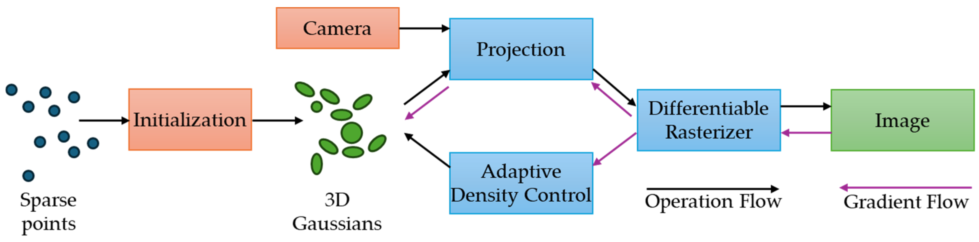
- Kerbl, B.; Kopanas, G.; Leimkuhler, T.; Drettakis, G. 3D Gaussian Splatting for Real-Time Radiance Field Rendering. ACM Trans. Graph. 2023, 42, 139. [Google Scholar] [CrossRef]
- Santosh Reddy, P.; Abhiram, H.; Archish, K.S. A Survey of 3D Gaussian Splatting: Optimization Techniques, Applications, and AI-Driven Advancements. In Proceedings of the 2025 International Conference on Intelligent and Innovative Technologies in Computing, Electrical and Electronics (IITCEE), Bangalore, India, 16–17 January 2025. [Google Scholar] [CrossRef]
- Qiu, S.; Xie, B.; Liu, Q.; Heng, P.-A. Creating Virtual Environments with 3D Gaussian Splatting: A Comparative Study. In Proceedings of the 2025 IEEE Conference on Virtual Reality and 3D User Interfaces Abstracts and Workshops (VRW), Saint Malo, France, 8–12 March 2025. [Google Scholar] [CrossRef]
- Hornáček, M.; Rozinaj, G. Exploring 3D Gaussian Splatting: An Algorithmic Perspective. In Proceedings of the 2024 International Symposium ELMAR, Zadar, Croatia, 16–18 September 2024. [Google Scholar] [CrossRef]
- Rosique, F.; Navarro, P.J.; Fernández, C.; Padilla, A. A Systematic Review of Perception System and Si-mulators for Autonomous Vehicles Research. Sensors 2019, 19, 648. [Google Scholar] [CrossRef]
- Elster, L.; Staab, J.P.; Peters, S. Making Automotive Radar Sensor Validation Measurements Comparable. Appl. Sci. 2023, 13, 11405. [Google Scholar] [CrossRef]
- Roy, C.J.; Balch, M.S. A Holistic Approach to Uncertainty Quantification with Application to Supersonic Nozzle Thrust. Int. J. Uncertain. Quantif. 2021, 2, 363–381. [Google Scholar] [CrossRef]
- Magosi, Z.F.; Eichberger, A. A Novel Approach for Simulation of Automotive Radar Sensors Designed for Systematic Support of Vehicle Development. Sensors 2023, 23, 3227. [Google Scholar] [CrossRef] [PubMed]
- Maier, M.; Makkapati, V.P.; Horn, M. Adapting Phong into a Simulation for Stimulation of Automotive Radar Sensors. In Proceedings of the 2018 IEEE MTT-S International Conference on Microwaves for Intelligent Mobility (ICMIM), Munich, Germany, 15–17 April 2018; pp. 1–4. [Google Scholar] [CrossRef]
- Minin, I.V.; Minin, O.V. Lens Candidates to Antenna Array. In Basic Principles of Fresnel Antenna Arrays; Lecture Notes Electrical Engineering; Springer: Berlin/Heidelberg, Germany, 2008; Volume 19, pp. 71–127. [Google Scholar] [CrossRef]
- Sensors Partners. LiDAR Laser: What Is LiDAR and How Does It Work?|Sensor Partners. Available online: https://sensorpartners.com/en/knowledge-base/how-a-lidar-laser-works/ (accessed on 6 March 2025).
- García-Gómez, P.; Royo, S.; Rodrigo, N.; Casas, J.R. Geometric Model and Calibration Method for a Solid-State LiDAR. Sensors 2020, 20, 2898. [Google Scholar] [CrossRef] [PubMed]
- Kim, G. Performance Index for Extrinsic Calibration of LiDAR and Motion Sensor for Mapping and Localization. Sensors 2022, 22, 106. [Google Scholar] [CrossRef] [PubMed]
- Schmoll, L.; Kemper, H.; Hagenmüller, S.; Brown, C.L. Validation of an Ultrasonic Sensor Model for Application in a Simulation Platform. ATZelectronics Worldw. 2024, 19, 8–13. [Google Scholar] [CrossRef]
- Stevens Institude of Thechnology 1870. Available online: https://www.stevens.edu/news/autonomous-vehicles-will-add-us81-billion-new-premiums-auto-insurers-2025-according-accenture-report (accessed on 18 May 2025).
- Sen, S.; Husom, E.J.; Goknil, A.; Tverdal, S.; Nguyen, P. Uncertainty-Aware Virtual Sensors for Cyber-Physical Systems. IEEE Softw. 2024, 41, 77–87. [Google Scholar] [CrossRef]
- Ying, Z.; Wang, Y.; He, Y.; Wang, J. Virtual Sensing Techniques for Nonlinear Dynamic Processes Using Weighted Proba-bility Dynamic Dual-Latent Variable Model and Its Industrial Applications. Knowl.-Based Syst. 2022, 235, 107642. [Google Scholar] [CrossRef]
- Yuan, X.; Rao, J.; Wang, Y.; Ye, L.; Wang, K. Virtual Sensor Modeling for Nonlinear Dynamic Processes Based on Local Weighted PSFA. IEEE Sens. J. 2022, 22, 20655–20664. [Google Scholar] [CrossRef]
- Zheng, T. Algorithmic Sensing: A Joint Sensing and Learning Perspective. In Proceedings of the 21st Annual International Conference on Mobile Systems, Applications and Services, Helsinki, Finland, 18–22 June 2023; Association for Computing Machinery: New York, NY, USA, 2023; pp. 624–626. [Google Scholar] [CrossRef]
- Es-haghi, M.S.; Anitescu, C.; Rabczuk, T. Methods for Enabling Real-Time Analysis in Digital Twins: A Literature Review. Comput. Struct. 2024, 297, 107342. [Google Scholar] [CrossRef]
- EUR-Lex, UN Regulation No 157—Uniform Provisions Concerning the Approval of Vehicles with Regards to Automated Lane Keeping Systems [2021/389]. Available online: https://eur-lex.europa.eu/eli/reg/2021/389/oj/eng (accessed on 18 May 2025).
- EUR-Lex, Regulation No 140 of the Economic Commission for Europe of the United Nations (UN/ECE)—Uniform Provisions Concerning the Approval of Passenger Cars with Regard to Electronic Stability Control (ESC) Systems [2018/1592]. Available online: https://eur-lex.europa.eu/eli/reg/2018/1592/oj/eng (accessed on 18 May 2025).
- International Organization for Standardization. ISO 26262-1:2018(en) Road Vehicles—Functional Safety—Part 1: Vocabulary. Available online: https://www.iso.org/obp/ui/en/#iso:std:iso:26262:-1:ed-2:v1:en (accessed on 19 May 2025).
- International Organization for Standardization. ISO 34502:2022 Road Vehicles—Test Scenarios for Automated Driving Systems—Scenario Based Safety Evaluation Framework. Available online: https://www.iso.org/standard/78951.html (accessed on 19 May 2025).
- International Organization for Standardization. ISO 21448:2022(en); Road Vehicles—Safety of the Intended Functionality. Available online: https://www.iso.org/obp/ui/en/#iso:std:iso:21448:ed-1:v1:en (accessed on 19 May 2025).


| Level 1 | Level 2 | Level 3 | Level 4 | Level 5 (Estimate) | |||||
|---|---|---|---|---|---|---|---|---|---|
| Model | Units | Model | Units | Model | Units | Model | Units | Model | Units |
| Ultrasonic | 4 | Ultrasonic | 8 | Ultrasonic | 8 | Ultrasonic | 8 | Ultrasonic | 10 |
| Radar long range | 1 | Radar long range | 1 | Radar long range | 2 | Radar long range | 2 | Radar long range | 2 |
| Radar short range | 2 | Radar short range | 4 | Radar short range | 4 | Radar short range | 4 | Radar short range | 4 |
| Camera mono | 1 | Camera mono | 4 | Camera mono | 2 | Camera mono | 3 | Camera mono | 3 |
| - | - | - | - | Camera stereo | 1 | Camera stereo | 1 | Camera stereo | 2 |
| - | - | - | - | Infra-red | 1 | Infra-red | 1 | Infra-red | 2 |
| - | - | - | - | Lidar 2D/3D | 1 | Lidar 2D/3D | 4 | Lidar 2D/3D | 4 |
| - | - | - | - | Global navigation | 1 | Global navigation | 1 | Global navigation | 1 |
| Total | 8 | Total | 17 | Total | 20 | Total | 24 | Total | 28 |
| 2012 | 2016 | 2018 | 2020 | Estimated by 2030 | |||||
| Function | LK | LDW | AD | SD | EM | FC | WLD | PT |
|---|---|---|---|---|---|---|---|---|
| Road curvature | ||||||||
| Longitudinal/lateral slope | ||||||||
| Deviation angle/distance | ||||||||
| Lane information | ||||||||
| Road point position | ||||||||
| Road marker attributes |
Disclaimer/Publisher’s Note: The statements, opinions and data contained in all publications are solely those of the individual author(s) and contributor(s) and not of MDPI and/or the editor(s). MDPI and/or the editor(s) disclaim responsibility for any injury to people or property resulting from any ideas, methods, instructions or products referred to in the content. |
© 2025 by the authors. Licensee MDPI, Basel, Switzerland. This article is an open access article distributed under the terms and conditions of the Creative Commons Attribution (CC BY) license (https://creativecommons.org/licenses/by/4.0/).
Share and Cite
Barabás, I.; Iclodean, C.; Beles, H.; Antonya, C.; Molea, A.; Scurt, F.B. An Approach to Modeling and Developing Virtual Sensors Used in the Simulation of Autonomous Vehicles. Sensors 2025, 25, 3338. https://doi.org/10.3390/s25113338
Barabás I, Iclodean C, Beles H, Antonya C, Molea A, Scurt FB. An Approach to Modeling and Developing Virtual Sensors Used in the Simulation of Autonomous Vehicles. Sensors. 2025; 25(11):3338. https://doi.org/10.3390/s25113338
Chicago/Turabian StyleBarabás, István, Calin Iclodean, Horia Beles, Csaba Antonya, Andreia Molea, and Florin Bogdan Scurt. 2025. "An Approach to Modeling and Developing Virtual Sensors Used in the Simulation of Autonomous Vehicles" Sensors 25, no. 11: 3338. https://doi.org/10.3390/s25113338
APA StyleBarabás, I., Iclodean, C., Beles, H., Antonya, C., Molea, A., & Scurt, F. B. (2025). An Approach to Modeling and Developing Virtual Sensors Used in the Simulation of Autonomous Vehicles. Sensors, 25(11), 3338. https://doi.org/10.3390/s25113338