1. Introduction
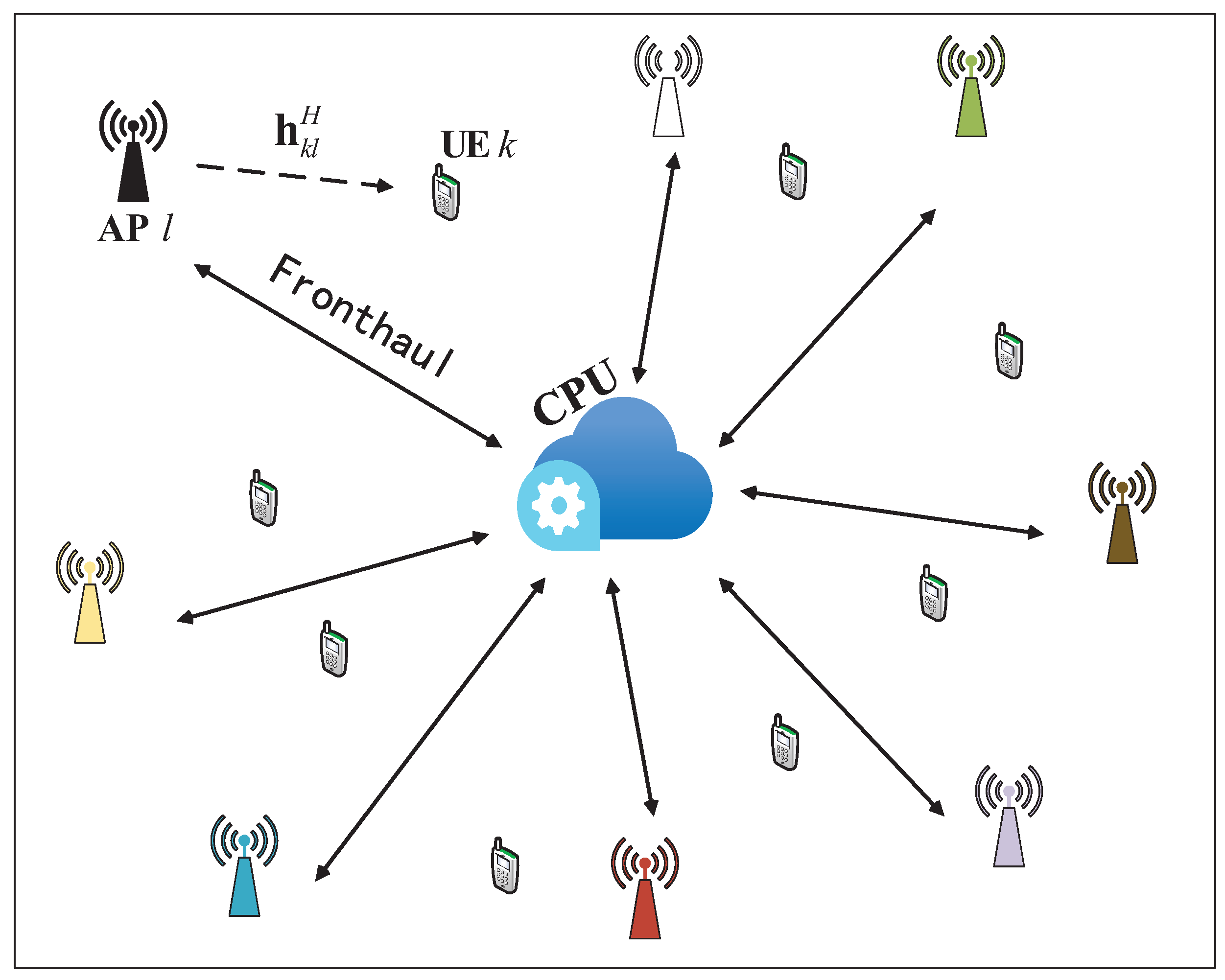
Cell-free mMIMO has gained significant attention due to its ability to provide universally good service to UEs, and it is regarded as a key technology for driving the development of 6G in the future. Traditional cellular mMIMO, which relies on cell division, often results in poor signal quality for edge UEs, while spectral efficiency progressively declines as the cell coverage area expands. In contrast, in a cell-free mMIMO system, numerous distributed APs are deployed near the UEs, with each AP equipped with a small number of antennas. All APs are connected to a central processing unit (CPU) responsible for handling all signals via wired or wireless fronthaul links. The APs collaborate to coherently transmit/receive signals for the UE, thereby reducing the interference issues faced by users at the cell edge. Since each UE is mainly influenced by the signals from nearby APs, this cell-free mMIMO system composed of numerous APs is also referred to as a user-centric network. This system architecture fully leverages the advantages of macro diversity, enhancing the overall system SE and ensuring a uniform quality of service for UEs [
1,
2].
As research deepens, the acquisition and optimization of CSI have become increasingly critical in cell-free mMIMO systems. The performance of such systems heavily depends on accurate CSI estimation. However, existing CSI estimation methods often suffer from high computational complexity and poor scalability in large-scale networks. In large systems, traditional CSI acquisition techniques typically involve extensive data exchange and complex computations, which consume substantial computational resources and degrade real-time processing capabilities, thereby limiting system performance. Particularly in uncertain channel environments, the robustness and efficiency of beamforming algorithms face significant challenges [
3,
4]. Therefore, there is an urgent need for new methods to address the complexity and scalability issues in CSI acquisition, thereby enhancing the adaptability and intelligence of the overall system [
5].
1.1. Related Work
In cell-free mMIMO systems, CSI is crucial for optimizing system performance. The system can generally be categorized into three types based on the level of collaboration between APs as folllows: distributed [
6,
7], centralized [
8,
9,
10], and semi-distributed large-scale fading (LSF) processing [
11]. In a centralized system, the instantaneous CSI of the whole network is collected at the CPU, which is used to suppress interference among the UEs. In [
9], the authors designed a near-optimal max–min fairness (MMF) power allocation method for centralized zero-forcing (ZF) precoding by iteratively maximizing the minimum SE of all UEs, and they combined this with a low complexity heuristic scheme. In [
12], the author proposed a centralized minimum mean square error (MMSE) precoding scheme and its joint power optimization strategy. The author proved that the centralized MMSE precoding can provide higher SE than centralized ZF precoding. Although the centralized scheme can effectively suppress inter-user interference and improve spectral efficiency, it relies on the CPU to conduct the signal processing and channel estimation of the entire network. In contrast, distributed techniques offload the signal processing task to distributed APs by using local CSI. In [
13], full-pilot ZF (FZF) precoding was proposed to eliminate the interference between UEs using local CSI at the APs, but the actual performance of the system is determined by the quantity of antenna arrays at each AP. To alleviate this constraint, local partial ZF (LP-ZF) precoding was proposed in [
14] by allowing each AP to reduce its interference to the strongest UEs. In [
10], the authors proposed a local partial MMSE (LP-MMSE) precoding to suppress inter-UE interference using UL-DL duality at the APs, which greatly improves the system performance, and this scheme had no requirement on the number of antennas at the APs. Compared to FZF and LP-ZF, LP-MMSE offers greater flexibility. Although computing local CSI distributively at each AP can avoid the fronthaul consumption of sending local CSI to the CPU, the performance of the distributed approaches is far inferior to the centralized methods.
To reduce the performance gap between distributed and centralized schemes, researchers have proposed utilizing LSF processing techniques to enhance the performance of distributed solutions [
15,
16]. During LSF processing, the LSF weight calculations require network-wide statistical CSI at the CPU. Previous studies on LSF generally assumed perfect instantaneous CSI to obtain the required statistical CSI for LSF weights’ calculation [
11], but this is only an ideal state and is not feasible in practical applications. In [
17], the authors proposed computing statistical CSI by performing a weighted average of local channel estimates from each AP, which requires statistical CSI exchange between APs and CPU via fronthaul links. In [
18], a new method was proposed for estimating CSI at the CPU using uplink data information. Although this method can reduce the fronthaul CSI overhead introduced during the LSF processing, it was derived under the condition that all APs provide services to all UEs. The complexity of statistical CSI estimation for each UE gradually increases as the number of UEs keeps increasing. Thus, this method is not scalable to large-scale networks with numerous UEs. In addition, the authors in [
19] designed a distributed fractional power allocation (FPA-dis) strategy that relies on large-scale fading factors for maximum ratio (MR) precoding, and in the literature [
20], a generalized fractional power control (GFPA) algorithm was further proposed to extend it to other precoding schemes. However, the GFPA algorithm requires local CSI to be sent to the CPU for power control, which leads to significant statistical CSI overhead on the fronthaul links.
1.2. Contributions
In this research, we propose a scalable method to estimate the statistical CSI in a user-centric cell-free mMIMO system, where each AP only serves a subset of UEs within the system. The proposed method uses uplink data to blindly estimate the partial statistical CSI required for LSF processing or power control in fully distributed DL beamforming. It avoids the statistical CSI exchange between APs and CPU for LSF processing and distributed power control, thus significantly reducing the statistical CSI overhead on the fronthaul link while ensuring system scalability. The key contributions can be summarized as follows:
Under the user-centric model, we propose a method that utilizes UL data signals to blindly estimate the partial statistical CSI necessary for LSF schemes. This method can achieve spectral efficiency comparable to, or even better than, that of conventional schemes while being scalable to large-scale networks with numerous UEs.
We show that the scalable CSI estimation method proposed in this paper can also be used for distributed power control methods such as GFPA [
20]. By blindly estimating the required CSI using UL data, this approach attains approximately the same SE as the traditional full statistical CSI feedback, which significantly reduces the fronthaul overhead for CSI transmission.
The proposed power control and statistical channel estimation methods are scalable to large-scale networks with numerous UEs, as each AP only provides services for a subset of UEs, with limited computational complexity in a user-centric framework.
Notation: denotes conjugate; denotes transpose; denotes conjugate transpose; denotes Euclidean norm; the expectation operator is indicated by ; denotes the diagonal matrix; denotes an m-row n-column zero matrix; and is a identity matrix with N rows and N columns. denotes Complex Gaussian Distribution.
2. System Model
We consider a cell-free mMIMO system, as illustrated in
Figure 1, consisting of
K single-antenna UEs and
L APs that are randomly deployed across a specific area. Each AP is equipped with
N antennas, where
and
. Each AP connects to the CPU via a fronthaul link, allowing them to share CSI and data between them via the CPU. We choose the conventional time division duplex (TDD) operating mode [
10,
21]. Each channel coherence block is segmented into channel uses allocated for UL and DL communications. Specifically,
channel uses are assigned for channel estimation,
channel uses for UL data transmission, and
channel uses will be used for DL data transmission. The channel between AP
l and UE
k is represented by
, and satisfies the following:
where
is a matrix describing the correlation of channels between AP
l and UE
k at different spatial locations.
denotes the MMSE estimation of the channel
, and
is the error generated during the estimation process and satisfies the following:
where
is a matrix describing the covariance relationship between the channel estimation errors
.
To enable system scalability, we use the user-centric dynamic cooperative clustering (DCC) framework from [
10]. In this framework, each UE is served by a subset of APs that are chosen according to the best channel conditions. The set of APs serving UE
k is denoted by
, which is a subset of all
L APs. Conversely, each AP
l serves a set of UEs
. We establish the service relationship between UE
i and AP
l through the diagonal service association matrix
. We assume that if an AP is determined to serve a particular UE, it will utilize all of its available antennas for that UE. The value of the diagonal matrix
is determined as follows: If
, then
; otherwise,
. Let diagonal matrix
represent the service relationships between all APs and UE
k.
3. Uplink Data Transmission and Scalable Statistical CSI Estimation
In this section, we first introduce the LSF detection (LSFD) scheme for UL transmission and then propose a scalable approach for the blind estimation of the partial statistical CSI required for LSF schemes based on UL data signals. LSFD consists of two layers of data decoding processes, where local channel information at each AP is utilized for the first layer of local decoding. The signal received at AP
l can be formulated as follows:
where
represents the signal transmitted by UE
k, with signals from different UEs being mutually independent, and
is the additive noise at AP
l.
After AP
l integrates the data signals from all serving UEs, it processes these signals according to the local combining vectors
to generate a preliminary estimate of the uplink signal. The local signal for UE
k is estimated as follows:
Following the local combination process, each AP
l sends the estimated local signal values
to the CPU.
Upon obtaining the transmitted signal from each AP, the CPU will use the network-wide statistical CSI to generate the LSFD vector for the second layer decoding of each UE. The LSFD vector that CPU selected for UE
k is denoted by
. The CPU’s final estimation of the uplink data for UE
k is as follows:
The LSFD vector’s basic criteria are defined in [
11] as follows:
where
is the power of UE
i during UL data transmission. However, Equation (
6) is derived under the assumption that every AP serves all UEs. As the quantity of UEs increases, the computational complexity of this method tends to approach infinity. In reference [
18], a CSI estimation (CSIE) method is proposed based on Equation (
6). However, this method also apparently fails to meet the requirements of scalability.
Under the user-centric DCC framework, the scalable LSFD vector of UE
k can be obtained by the following equation:
where
is defined as the cluster of UEs that share the same APs with UE
k.
. In particular, note that
represents the combination of the combining vectors of UE
k with the channel vectors of UE
i.
is an
L-dimensional sparse vector, with an effective dimension of
(
denotes the cardinality of the set
);
is a sparse diagonal matrix, since when
, the matrix
; and the corresponding entries in
and
are zero. The all-zero columns/rows in
and
will be removed before the matrix inversion is taken. So Equation (
9) only needs to compute the inverse of a
matrix, while Equation (
6) needs to compute the inverse of a
matrix. Therefore, the computational complexity of Equation (
9) is much lower compared to Equation (
6).
Scalable Statistical CSI Estimation
From Equation (
9), it can be seen that when using the traditional method to compute
, the CPU needs to compute the complex matrix
and the complex vector
, and this requires each AP to send its locally estimated statistical CSI to the CPU via fronthaul links, which lead to CSI overhead in fronthaul. However, we can utilize the estimated UL signals from all APs, which are sent to the CPU, as shown in Equation (
4), as training data to blindly estimate
at the CPU. Let
,
represent the partial statistical CSI needed to compute the LSFD vector in Equation (
9).
Let
be the collective data signal from all UEs and
represent the estimated signal for UE
k. While all UEs transmit their signals, only the APs corresponding to
will actually estimate them. Thus, we have the following:
where
represents the equivalent channel matrix of UE
k, which is a
sparse matrix, with corresponding element
, when
.
is a sparse noise vector. Considering that the transmission signals of different UEs are independent, we have the following:
The correlation between the original transmission signal
from UE
k and its local estimate
, as illustrated in Equation (
4), can be written as follows:
Thus, we have:
During the
cth coherent block, when utilizing channel
t, we define
as the local estimation of the uplink data signal for UE
k. Throughout the entire coherent block,
is defined as the overall estimation of the uplink data signal for UE
k. Then,
can be estimated as follows:
where
C denotes the total number of coherent blocks.
We found that to calculate
, we need the actual UL data signal
sent by UE
k, which is unavailable to the CPU. However, the CPU can integrate the local estimation of UE
k’s transmitted signal at each AP in Equation (
4) to estimate
, which is given as follows:
Then, the CPU makes a decision on
to obtain the preliminary detection result
of the uplink data signal for UE
k. If the estimation error of UE
k at each AP is small, we can perfectly replace
with
, and we have the following:
Let
be the overall estimation of the UL data signal for UE
k at the
tth channel use during the
cth coherent block. In addition, let
represent the local estimation of the uplink signal from UE
k at AP
l during the
tth channel use of the
cth coherent block. Across all channel uses in the cth coherence block, we have
and
. Then,
can be expressed as follows:
From Equation (
17) and Equation (
20), we can directly estimate the LSFD vector
for UE
k as follows:
5. Performance Analysis
We use MATLAB-R2021b simulations to evaluate the effectiveness of the scheme presented in this work. We configured
APs and
UEs uniformly distributed over an area. Each AP boasts
antennas, while each UE relies on just one antenna. The maximum DL transmission power is
, and the channel bandwidth is 20 MHz. We consider two different scenarios as shown in
Table 2.
Figure 2 compares the cumulative distribution function (CDF) curves of the DL SE per UE corresponding to different power control algorithms under LSFP for CSIE-S, CSIE, and PCSIF in scenario 1. We consider the LP-MMSE precoding and three different power control strategies as listed in scenario 1 of
Table 2. it is evident that compared to the traditional non-scalable CSIE, the proposed CSIE-S method can achieve nearly the same SE performance under various power allocation algorithms while ensuring system scalability. Compared to PCSIF, CSIE-S avoids fronthaul overhead and achieves nearly the same SE performance, even attaining higher SE gains; for example, under the SPC power control scheme, CSIE-S significantly outperforms PCSIF. These results demonstrate the effectiveness and practicality of the CSIE-S method for DL LSFP.
Figure 3 compares the CDF curves corresponding to the downlink SE per UE in CSIE-S, CSIE, and PCSIF under the MFPA algorithm in scenario 1. We set up the following three different AP antenna configuration schemes in the simulation:
and 8, respectively. The simulation results show that, with the continuous increase of antenna deployment
N, the system’s spectral efficiency progressively improves. This improvement is attributed to the spatial diversity and multiplexing gain provided by numerous antennas. Multiple antenna arrays can transmit directionally to each UE and receive directionally from them. The multiplexing gain permits the system to send multiple data streams via different antennas simultaneously within the same frequency band, dramatically increasing the system’s capacity and SE. This improves the accuracy of signal detection to a certain extent, and it effectively reduces the interference between UEs. It is essential to emphasize that, regardless of the increase or decrease in the number of antennas, the scalable CSIE-S scheme has always maintained nearly similar performance to CSIE and PCSIF.
In the process of calculating statistical CSI, the complexity of the algorithm mainly arises from matrix inversion and the number of UEs involved. The complexity of CSIE and CSIE-S is summarized in
Table 3, using the number of complex multiplications. Here,
and
represent the cardinality of the sets
and
, respectively. Since the number of antennas
N equipped at each AP is limited, the complexity of CSIE gradually becomes unmanageable as the number of UEs and APs in the area increases. However, the complexity of CSIE-S only depends on the sets
and
. When
and
are constants, regardless of how the number of UEs and APs increases, CSIE-S maintains a finite complexity. Therefore, CSIE-S is more adaptable to large networks with a significant number of UEs and APs.
Figure 4,
Figure 5 and
Figure 6 compare the CDF curves corresponding to the downlink SE per UE under different distributed precoding schemes in scenario 2. We compared the performance of the GFPA-E algorithm proposed in this paper with the existing FPA-dis algorithm and the GFPA algorithm, where the parameters are all set to
and
. In addition, the MR [
10] scheme with the FPA-dis algorithm provides the lower performance limit, while the partial MMSE (P-MMSE) [
10] scheme with centralized equal power allocation (P-MMSE-EPA) provides the upper performance limit for the system. The results show that FPA-dis performs poorly. Among the three different precoding schemes, the proposed GFPA-E scheme achieves performance almost comparable to GFPA, and it even achieves higher SE gains at certain points (for example, in the lower tail portions of the CDF curves in
Figure 5 and
Figure 6). It is important to emphasize that GFPA-E avoids the additional fronthaul CSI overhead, as we derived, since GFPA-E relies on UL data to compute the equivalent large-scale fading channel factor involved in GFPA.
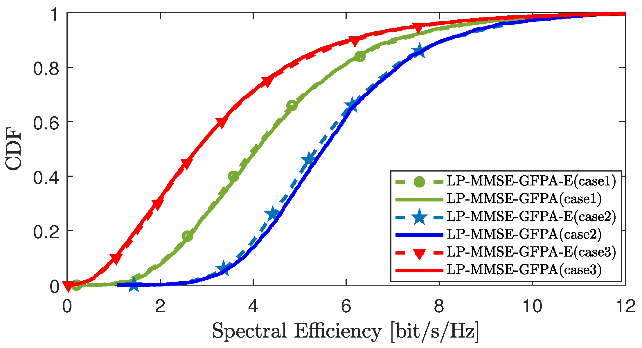
Figure 7 compares the CDF curves corresponding to the downlink SE per UE under the GFPA algorithm and the GFPA-E algorithm in scenario 2, where the parameters are set to
and
. We compared the following three different cases: Case 1,
; Case 2,
; and Case 3,
. The simulation results show that, with the continuous expansion of mobile UEs’ scale in the region, the SE performance of the GFPA and GFPA-E algorithms exhibits the typical multiuser degradation characteristics. This is mainly due to the fact that having more UEs sharing pilot resources exacerbates pilot contamination, thereby reducing channel estimation accuracy. On the contrary, the rise in the quantity of APs notably enhances the system’s performance, as more APs provide greater spatial diversity gain, which effectively suppresses inter-user interference. In addition, regardless of how the scale of UEs and APs changes, the GFPA-E solution achieves nearly similar performance to the GFPA.
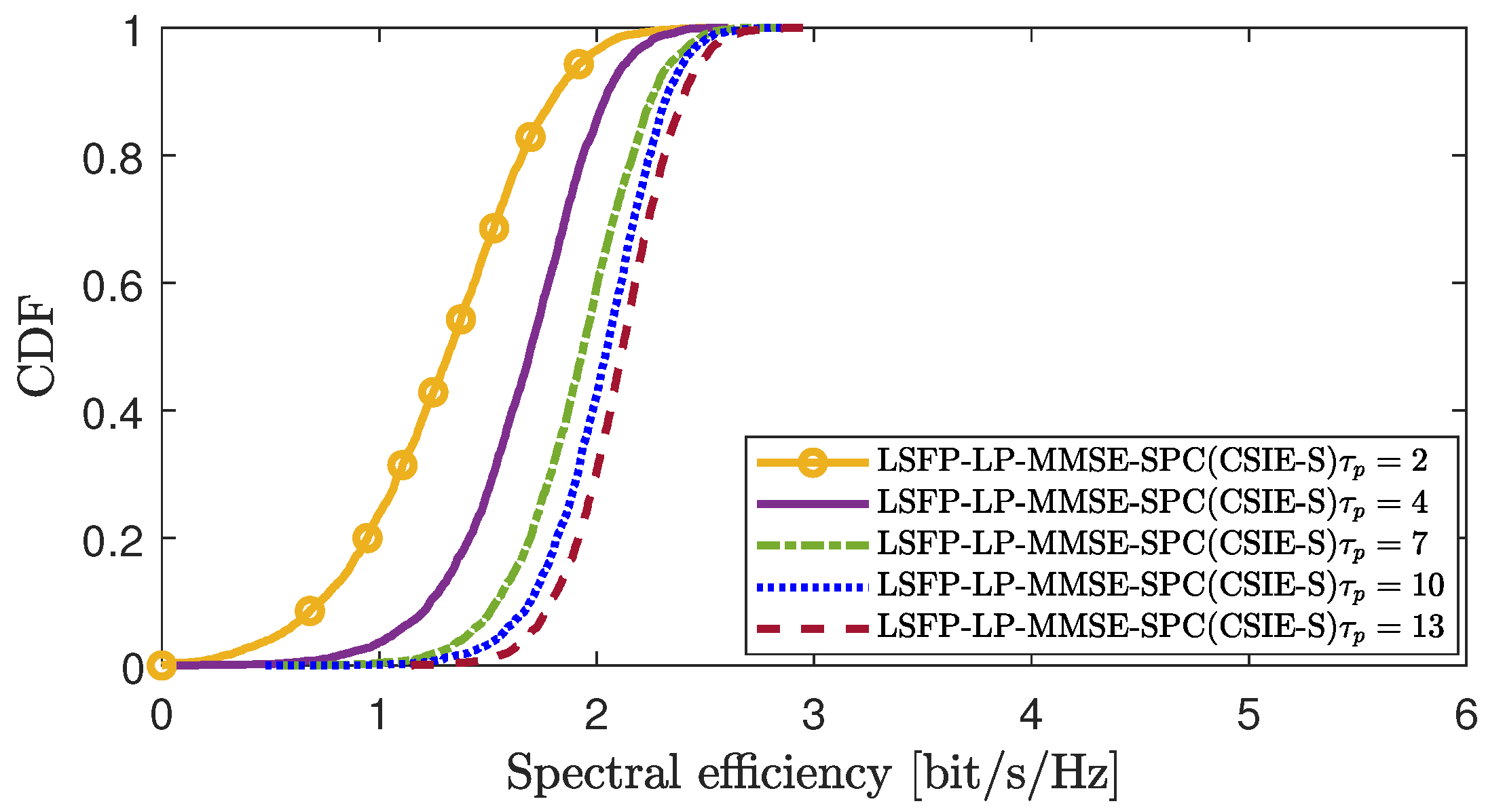
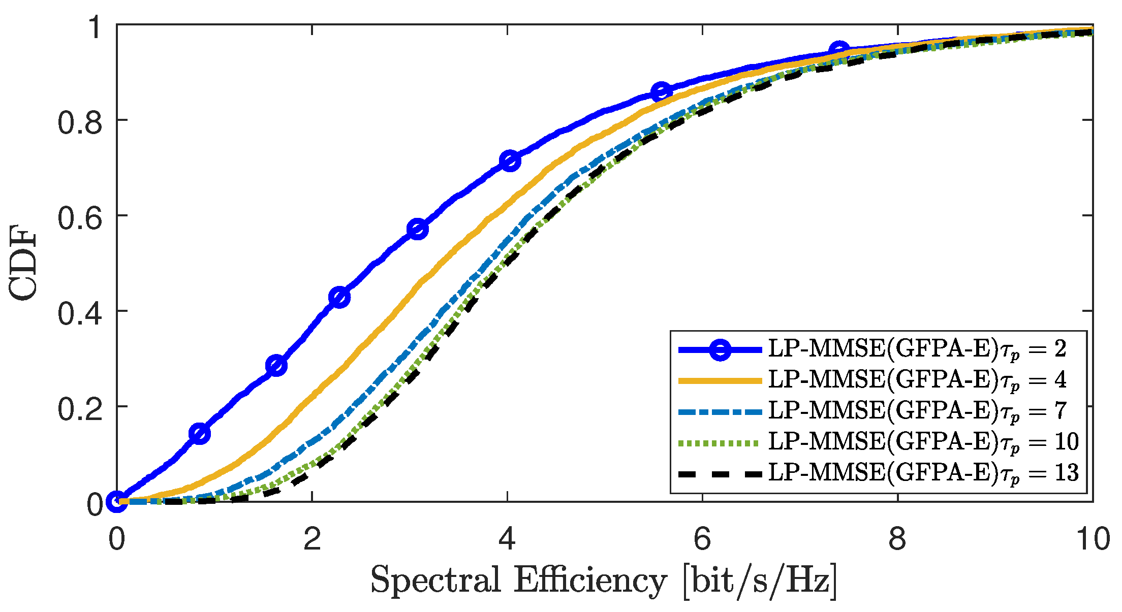
Figure 8 and
Figure 9 analyze the impact of pilot contamination or imperfect channel estimation on the performance of the proposed scheme in scenario 1 and scenario 2, respectively. A larger value of
indicates more abundant pilot resources, resulting in reduced pilot contamination and smaller channel estimation errors. From the figures, we can see that when the pilot resource
is very small, different UEs share the same pilot, leading to pilot contamination and inaccurate channel estimation, which degrades the overall performance of the system. As the pilot resource
gradually increases, the pilot contamination situation improves, enhancing the accuracy of channel estimation and thereby improving the system’s performance.
Figure 10 compares the impact on the DL SE per UE when different parameters are selected for GFPA-E in scenario 2. Parameters
and
are introduced to provide flexibility, allowing the system to balance between performance maximization and fairness. As shown in the figure, when
, UEs with poor channel conditions (i.e., the lower tail of the CDF curve) fail to receive effective power allocation, resulting in degraded performance for weak UEs. As
gradually increases, the performance of weak UEs gradually improves; and when
, the rise of the CDF curve is significantly faster, indicating improved fairness across the system. Under the same conditions, a larger
value is more favorable to system fairness, while a smaller
tends to allocate more power to UEs with better channel conditions. However, the overall system performance seems to be insensitive to the choice of parameters
and
. As long as the values are taken within a reasonable interval, the performance of GFPA-E is stable in different scenarios. This indicates that the method is robust and easy to use in terms of practical parameter settings.
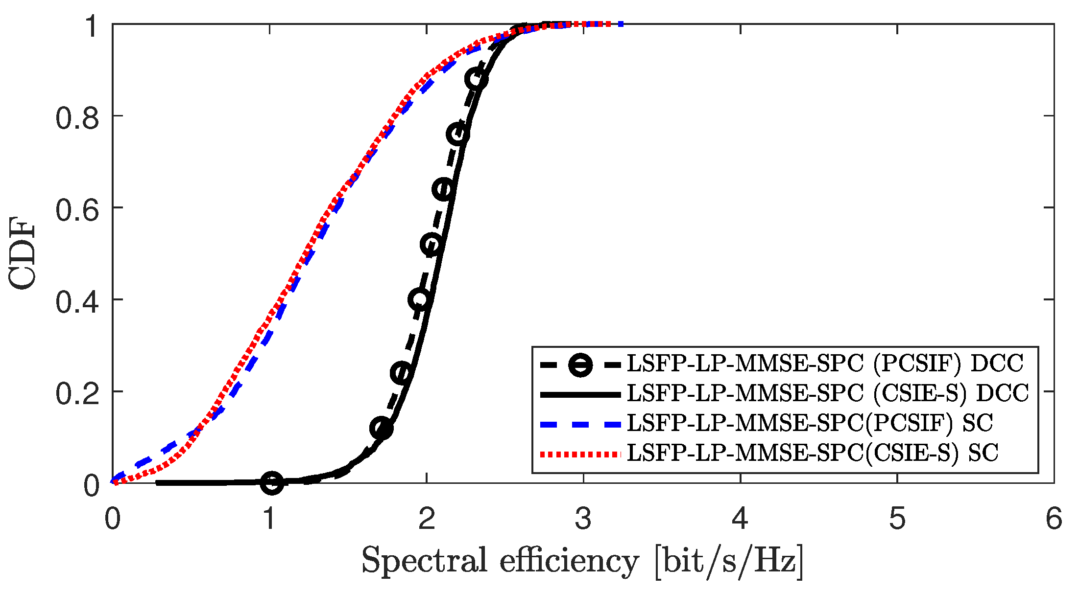
Figure 11 compares the performance of the proposed CSIE-S method with the conventional PCSIF method under different clustering strategies in scenario 1. To comprehensively evaluate the adaptability and robustness of the proposed algorithm across various clustering approaches, we consider not only the user-centric dynamic cooperative clustering (DCC) strategy proposed in [
10] but also introduce another suboptimal clustering (SC) method, as proposed in [
24]. In this method, each UE selects a fixed number of APs with the strongest channel conditions as its serving APs, without considering the effects of pilot contamination. Simulation results show that under both DCC and SC strategies, the CSIE-S method achieves comparable SE performance to the PCSIF scheme. However, the performance of the algorithm under the DCC strategy is significantly better than that under SC. This demonstrates that the CSIE-S method is not only applicable to DCC but also compatible with other clustering strategies, but its performance may vary slightly depending on the specific clustering method employed.


