
3D Micro-Expression Recognition Based on Adaptive Dynamic Vision

Abstract
1. Introduction
- (1)
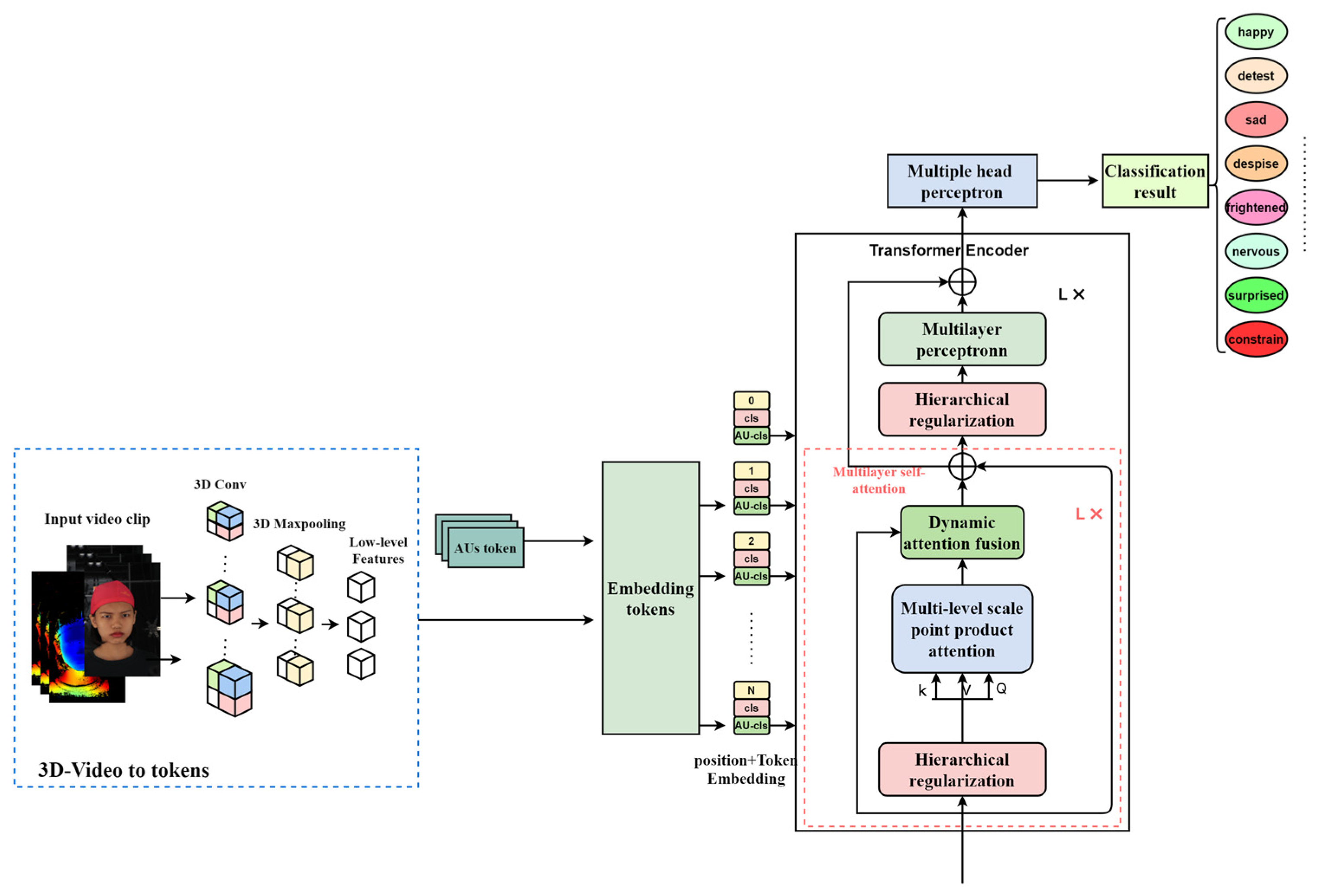
- We propose a novel deep learning DFER research paradigm, MADV-Net, for macro–micro-expression mixed data. By leveraging self-supervised fine-tuning models to learn sufficient global features, combined with fine-grained local feature learning strategies, we design a DFER paradigm model with high reliability and generalization capabilities.
- (2)
- The video stream data are divided into low-dimensional, middle-dimensional, and high-dimensional feature streams through the design of adaptive and dynamic partition feature extraction models, and the information on inter-frame differences is learned through dynamic adaptive factors. Finally, the pyramid structure fuses feature information streams for subsequent fine-grained recognition and classification.
- (3)
- The dual-channel attention model of AU coding and the image and video encoder are innovatively designed, and adaptive dynamic adjustment of feature information is skillfully used. The multi-level features are dynamically fused and output to the multi-level head perceptron. Then, a fine-grained classification function is used to accurately identify the emotions in the video stream in real time.
2. Related Work
2.1. Expression Recognition Algorithm Based on Visual Encoder
2.2. Micro-Expression Recognition Method Based on AU Coding
3. Proposed Method
3.1. Multi-Level Adaptive Dynamic Visual Attention Network Model Design
3.2. Video Feature Encoding Based on Adaptive Dynamic Regulation
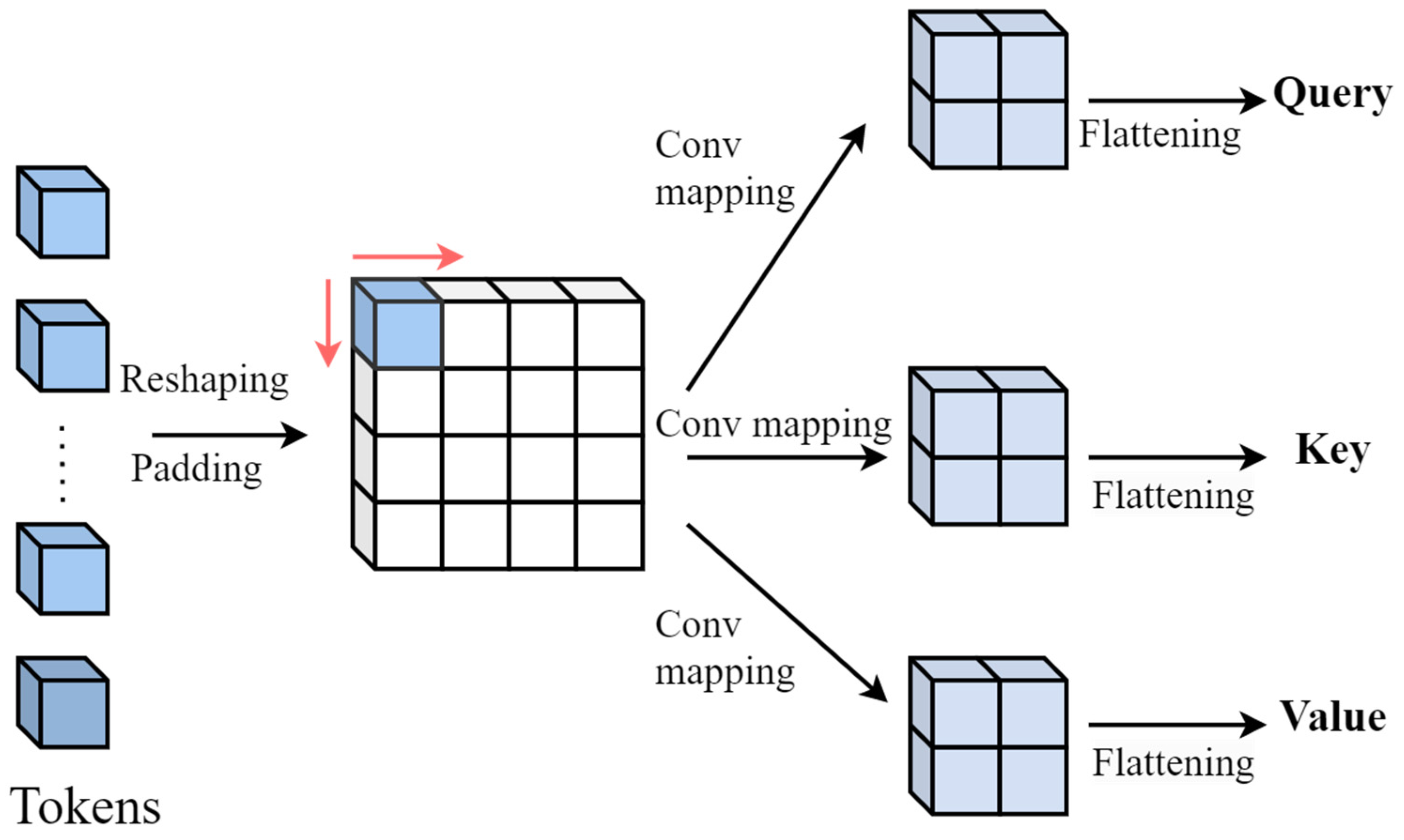
3.2.1. Deep Convolution Mapping
- 3D-video-to-tokens module
3.2.2. AU-Based Feature Coding Submodule
3.2.3. Adaptive Attention Adjustment
3.2.4. Loss Function
3.2.5. Algorithm Complexity
4. Experimental Setup and Experimental Results
4.1. Introduction of Dataset
4.2. Evaluation Index
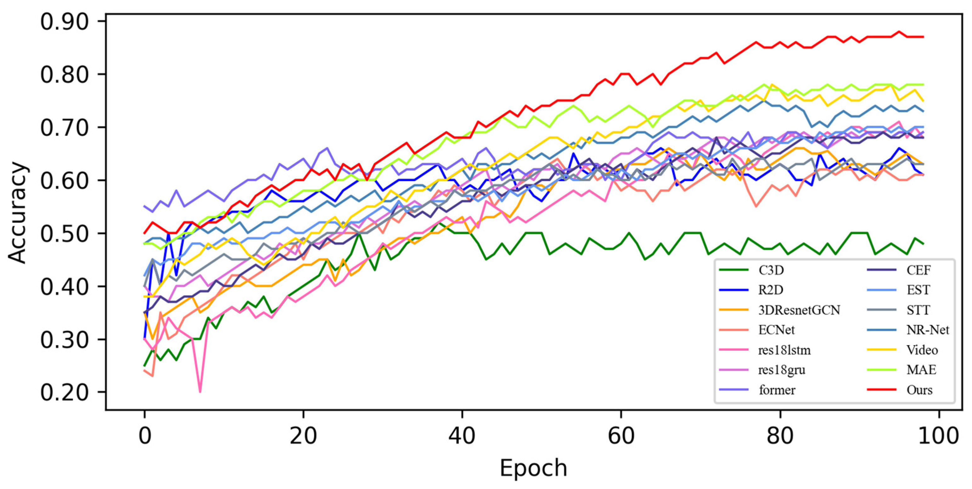
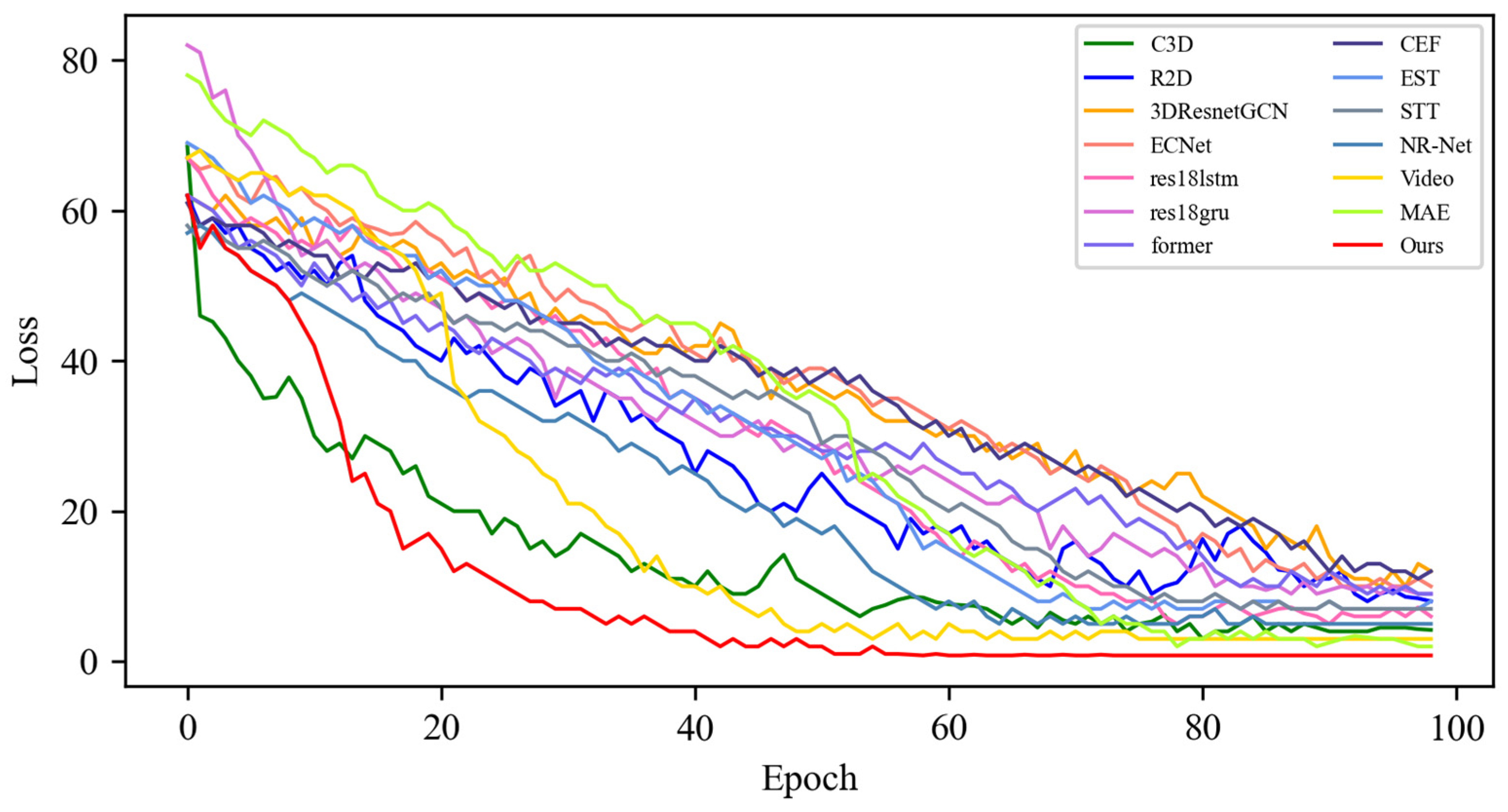
4.3. Contrast Experiment
4.3.1. Experimental Results on SMIC Dataset
4.3.2. Experimental Results on CASME-II Dataset
4.3.3. Experimental Results on CAS(ME)2 Dataset
4.3.4. Experimental Results on the SAMM Dataset
4.4. Quantitative Result Analysis
4.4.1. Experimental Results on SMIC Dataset
4.4.2. Experimental Results on CASME-II Dataset
4.4.3. Experimental Results on CAS(ME)2 Dataset
4.4.4. Experimental Results on SAMM Dataset
4.5. Visualization Experiment
5. Conclusions
Author Contributions
Funding
Institutional Review Board Statement
Informed Consent Statement
Data Availability Statement
Conflicts of Interest
Abbreviations
| MaE | Macro expression |
| ME | Micro expression |
| FER | Facial expression recognition |
| SFER | Static facial expression recognition |
| DFER | Dynamic facial expression recognition |
| AU | Action unit |
| MADV-Net | Multi-level adaptive dynamic visual attention network model |
| FACS | Facial Motion Coding System |
References
- Ge, H.; Zhu, Z.; Dai, Y.; Wang, B.; Wu, X. Facial Expression Recognition Based on Deep Learning. Comput. Methods Programs Biomed. 2022, 215, 106621. [Google Scholar] [CrossRef]
- Liong, G.B.; Liong, S.T.; See, J.; Chan, C.S. MTSN: A Multi-Temporal Stream Network for Spotting Facial Macro- and Micro-Expression with Hard and Soft Pseudo-Labels. In Proceedings of the 2nd Workshop on Facial Micro-Expression: Advanced Techniques for Multi-Modal Facial Expression Analysis, Lisbon, Portugal, 14 October 2022. [Google Scholar]
- Li, J.; Yap, M.H.; Cheng, W.H.; See, J.; Hong, X.; Li, X.; Wang, S.J.; Davison, A.K.; Li, Y.; Dong, Z. MEGC2022: ACM Multimedia 2022 Micro-Expression Grand Challenge. In Proceedings of the 30th ACM International Conference on Multimedia, Lisbon, Portugal, 10 October 2022. [Google Scholar]
- Canal, F.Z.; Müller, T.R.; Matias, J.C.; Scotton, G.G.; de Sa Junior, A.R.; Pozzebon, E.; Sobieranski, A.C. A Survey on Facial Emotion Recognition Techniques: A State-of-the-Art Literature Review. Inf. Sci. 2022, 582, 593–617. [Google Scholar] [CrossRef]
- Wang, H.; Li, B.; Wu, S.; Shen, S.; Liu, F.; Ding, S.; Zhou, A. Rethinking the Learning Paradigm for Dynamic Facial Expression Recognition. In Proceedings of the IEEE/CVF Conference on Computer Vision and Pattern Recognition, Vancouver, BC, Canada, 27–30 June 2023. [Google Scholar]
- Chumachenko, K.; Iosifidis, A.; Gabbouj, M. MMA-DFER: MultiModal Adaptation of Unimodal Models for Dynamic Facial Expression Recognition in-the-Wild. In Proceedings of the IEEE/CVF Conference on Computer Vision and Pattern Recognition, Seattle, WA, USA, 17–22 June 2024. [Google Scholar]
- Han, Z.; Meichen, X.; Hong, P.; Zhicai, L.; Jun, G. NSNP-DFER: A Nonlinear Spiking Neural P Network for Dynamic Facial Expression Recognition. Comput. Electr. Eng. 2024, 115, 109125. [Google Scholar] [CrossRef]
- Liu, F.; Wang, H.; Shen, S. Robust Dynamic Facial Expression Recognition. IEEE Trans. Biometr. Behav. Ident. Sci. 2025, 7, 1–12. [Google Scholar] [CrossRef]
- Zhang, Y.; Zhang, J.; Shen, L.; Yu, Z.; Gao, Z. Fine-Grained Temporal-Enhanced Transformer for Dynamic Facial Expression Recognition. IEEE Signal Process. Lett. 2024, 31, 1–5. [Google Scholar] [CrossRef]
- Varanka, T.; Peng, W.; Zhao, G. Learnable Eulerian Dynamics for Micro-Expression Action Unit Detection. In Proceedings of the Scandinavian Conference on Image Analysis, Trondheim, Norway, 18–20 April 2023. [Google Scholar]
- Zhu, L.; He, Y.; Yang, X.; Li, H.; Long, X. Micro-Expression Recognition Based on Euler Video Magnification and 3D Residual Network under Imbalanced Sample. Eng. Res. Express 2024, 6, 035208. [Google Scholar] [CrossRef]
- Li, X.; Pfister, T.; Huang, X.; Zhao, G.; Pietikäinen, M. A Spontaneous Micro-Expression Database: Inducement, Collection and Baseline. In Proceedings of the 10th IEEE International Conference and Workshops on Automatic Face and Gesture Recognition (FG), Shanghai, China, 22–26 April 2013. [Google Scholar]
- Yan, W.J.; Li, X.; Wang, S.J.; Zhao, G.; Liu, Y.J.; Chen, Y.H.; Fu, X. CASME II: An Improved Spontaneous Micro-Expression Database and the Baseline Evaluation. PLoS ONE 2014, 9, e86041. [Google Scholar] [CrossRef]
- Qu, F.; Wang, S.J.; Yan, W.J.; Li, H.; Wu, S.; Fu, X. CAS (ME)2: A Database for Spontaneous Macro-Expression and Micro-Expression Spotting and Recognition. IEEE Trans. Affect. Comput. 2017, 9, 424–436. [Google Scholar] [CrossRef]
- Davison, A.K.; Lansley, C.; Costen, N.; Tan, K.; Yap, M.H. SAMM: A Spontaneous Micro-Facial Movement Dataset. IEEE Trans. Affect. Comput. 2016, 9, 116–129. [Google Scholar] [CrossRef]
- Yuan, L.; Chen, Y.; Wang, T.; Yu, W.; Shi, Y.; Jiang, Z.H.; Tay, F.E.; Feng, J.; Yan, S. Tokens-to-Token ViT: Training Vision Transformers From Scratch on ImageNet. In Proceedings of the IEEE/CVF International Conference on Computer Vision, Montreal, QC, Canada, 11–17 October 2021; pp. 558–567. [Google Scholar]
- Yin, H.; Vahdat, A.; Alvarez, J.M.; Mallya, A.; Kautz, J.; Molchanov, P. A-ViT: Adaptive Tokens for Efficient Vision Transformer. In Proceedings of the IEEE/CVF Conference on Computer Vision and Pattern Recognition, New Orleans, LA, USA, 18–24 June 2022; pp. 10809–10818. [Google Scholar]
- Yang, Y.; Hu, L.; Zu, C.; Zhang, J.; Hou, Y.; Chen, Y.; Zhou, J.; Zhou, L.; Wang, Y. CL-TransFER: Collaborative Learning Based Transformer for Facial Expression Recognition with Masked Reconstruction. Pattern Recognit. 2024, 156, 110741. [Google Scholar] [CrossRef]
- Nagarajan, P.; Kuriakose, G.R.; Mahajan, A.D.; Karuppasamy, S.; Lakshminarayanan, S. Emotion Recognition from Videos Using Transformer Models. In Computational Vision and Bio-Inspired Computing: Proceedings of ICCVBIC 2022; Springer Nature: Singapore, 2023; pp. 45–56. [Google Scholar]
- Arnab, A.; Dehghani, M.; Heigold, G.; Sun, C.; Lučić, M.; Schmid, C. ViViT: A Video Vision Transformer. In Proceedings of the IEEE/CVF International Conference on Computer Vision, Montreal, QC, Canada, 11–17 October 2021; pp. 6836–6846. [Google Scholar]
- Higashi, T.; Ishibashi, R.; Meng, L. ViViT Fall Detection and Action Recognition. In Proceedings of the 2024 International Conference on Advanced Mechatronic Systems (ICAMechS), Dalian, China, 26–28 November 2024; IEEE: Piscataway, NJ, USA, 2024; pp. 291–296. [Google Scholar]
- Kobayashi, T.; Seo, M. Efficient Compression Method in Video Reconstruction Using Video Vision Transformer. In Proceedings of the 2024 IEEE 13th Global Conference on Consumer Electronics (GCCE), Shenzhen, China, 29–31 October 2024; IEEE: Piscataway, NJ, USA, 2024; pp. 724–725. [Google Scholar]
- Deng, F.; Yang, C.; Guo, H.; Wang, Y.; Xu, L. DA-ViViT: Fatigue Detection Framework Using Joint and Facial Keypoint Features with Dynamic Distributed Attention Video Vision Transformer. Unpublished Work. 2024. [Google Scholar]
- Bargshady, G.; Joseph, C.; Hirachan, N.; Goecke, R.; Rojas, R.F. Acute Pain Recognition from Facial Expression Videos Using Vision Transformers. In Proceedings of the 2024 46th Annual International Conference of the IEEE Engineering in Medicine and Biology Society (EMBC), Singapore, 15–19 July 2024; IEEE: Piscataway, NJ, USA, 2024; pp. 1–4. [Google Scholar]
- Essa, I.A.; Pentland, A.P. Coding, Analysis, Interpretation, and Recognition of Facial Expressions. IEEE Trans. Pattern Anal. Mach. Intell. 1997, 19, 757–763. [Google Scholar] [CrossRef]
- Krumhuber, E.G.; Skora, L.I.; Hill, H.C.; Lander, K. The Role of Facial Movements in Emotion Recognition. Nat. Rev. Psychol. 2023, 2, 283–296. [Google Scholar] [CrossRef]
- Dong, Z.; Wang, G.; Lu, S.; Li, J.; Yan, W.; Wang, S.J. Spontaneous Facial Expressions and Micro-Expressions Coding: From Brain to Face. Front. Psychol. 2022, 12, 784834. [Google Scholar] [CrossRef] [PubMed]
- Buhari, A.M.; Ooi, C.P.; Baskaran, V.M.; Phan, R.C.; Wong, K.; Tan, W.H. FACS-based graph features for real-time micro-expression recognition. J. Imaging 2020, 6, 130. [Google Scholar] [CrossRef] [PubMed]
- Zhang, W.; Qiu, F.; Wang, S.; Zeng, H.; Zhang, Z.; An, R.; Ma, B.; Ding, Y. Transformer-Based Multimodal Information Fusion for Facial Expression Analysis. In Proceedings of the IEEE/CVF Conference on Computer Vision and Pattern Recognition, New Orleans, LA, USA, 18–24 June 2022; pp. 2428–2437. [Google Scholar]
- Savchenko, A.V.; Savchenko, L.V.; Makarov, I. Classifying Emotions and Engagement in Online Learning Based on a Single Facial Expression Recognition Neural Network. IEEE Trans. Affect. Comput. 2022, 13, 2132–2143. [Google Scholar] [CrossRef]
- Nga, C.H.; Vu, D.Q.; Le, P.T.; Luong, H.H.; Wang, J.C. MLSS: Mandarin English Code-Switching Speech Recognition Via Mutual Learning-Based Semi-Supervised Method. IEEE Signal Process. Lett. 2025, 32, 1–5. [Google Scholar] [CrossRef]
- Belharbi, S.; Pedersoli, M.; Koerich, A.L.; Bacon, S.; Granger, E. Guided Interpretable Facial Expression Recognition via Spatial Action Unit Cues. In Proceedings of the 2024 IEEE 18th International Conference on Automatic Face and Gesture Recognition (FG), Istanbul, Turkey, 27–31 May 2024; IEEE: Piscataway, NJ, USA, 2024; pp. 1–10. [Google Scholar]
- An, R.; Jin, A.; Chen, W.; Zhang, W.; Zeng, H.; Deng, Z.; Ding, Y. Learning Facial Expression-Aware Global-to-Local Representation for Robust Action Unit Detection. Appl. Intell. 2024, 54, 1405–1425. [Google Scholar] [CrossRef]
- Chang, D.; Yin, Y.; Li, Z.; Tran, M.; Soleymani, M. LibreFace: An Open-Source Toolkit for Deep Facial Expression Analysis. In Proceedings of the IEEE/CVF Winter Conference on Applications of Computer Vision, Salt Lake City, UT, USA, 18–21 March 2024; pp. 8205–8215. [Google Scholar]
- Chen, Y.; Zhong, C.; Huang, P.; Cai, W.; Wang, L. Improving Micro-Expression Recognition using Multi-sequence Driven Face Generation. In Proceedings of the 2025 IEEE International Conference on Acoustics, Speech and Signal Processing (ICASSP), Shanghai, China, 6–10 April 2025; IEEE: Piscataway, NJ, USA, 2025; pp. 1–5. [Google Scholar]
- Yang, L.; Kang, B.; Huang, Z.; Xu, X.; Feng, J.; Zhao, H. Depth anything: Unleashing the power of large-scale unlabeled data. In Proceedings of the IEEE/CVF Conference on Computer Vision and Pattern Recognition, Seattle, WA, USA, 16–22 June 2024. [Google Scholar]
- Pan, H.; Xie, L.; Wang, Z. C3DBed: Facial Micro-Expression Recognition With Three-Dimensional Convolutional Neural Network Embedding in Transformer Model. Eng. Appl. Artif. Intell. 2023, 123, 106258. [Google Scholar] [CrossRef]
- Han, X.; Lu, F.; Yin, J.; Tian, G.; Liu, J. Sign Language Recognition Based on R(2+1)D With Spatial–Temporal–Channel Attention. IEEE Trans. Hum.-Mach. Syst. 2022, 52, 687–698. [Google Scholar] [CrossRef]
- Al-Khater, W.; Al-Madeed, S. Using 3D-VGG-16 and 3D-Resnet-18 Deep Learning Models and FABEMD Techniques in the Detection of Malware. Alex. Eng. J. 2024, 89, 39–52. [Google Scholar] [CrossRef]
- Gong, W.; Qian, Y.; Zhou, W.; Leng, H. Enhanced Spatial-Temporal Learning Network for Dynamic Facial Expression Recognition. Biomed. Signal Process. Control 2024, 88, 105316. [Google Scholar] [CrossRef]
- Guo, Z.; Wang, J.; Zhang, B.; Ku, Y.; Ma, F. A Dual Transfer Learning Method Based on 3D-CNN and Vision Transformer for Emotion Recognition. Appl. Intell. 2025, 55, 200. [Google Scholar] [CrossRef]
- Ni, R.; Jiang, H.; Zhou, L.; Lu, Y. Lip Recognition Based on Bi-GRU With Multi-Head Self-Attention. In Proceedings of the IFIP International Conference on Artificial Intelligence Applications and Innovations, Corfu Greece, 27–30 June 2024; Springer Nature: Cham, Switzerland, 2024; pp. 99–110. [Google Scholar]
- Zhao, Z.; Liu, Q. Former-DFER: Dynamic Facial Expression Recognition Transformer. In Proceedings of the 29th ACM International Conference on Multimedia, Virtual Event, 20–24 October 2021; pp. 1553–1561. [Google Scholar]
- Li, Y.; Xi, M.; Jiang, D. Cross-View Adaptive Graph Attention Network for Dynamic Facial Expression Recognition. Multimed. Syst. 2023, 29, 2715–2728. [Google Scholar] [CrossRef]
- Gao, Y.; Su, R.; Ben, X.; Chen, L. EST Transformer: Enhanced Spatiotemporal Representation Learning for Time Series Anomaly Detection. J. Intell. Inf. Syst. 2025, 1–23. [Google Scholar] [CrossRef]
- Khan, M.; El Saddik, A.; Deriche, M.; Gueaieb, W. STT-Net: Simplified Temporal Transformer for Emotion Recognition. IEEE Access 2024, 12, 86220–86231. [Google Scholar] [CrossRef]
- Gera, D.; Raj Kumar, B.V.; Badveeti, N.S.; Balasubramanian, S. Dynamic Adaptive Threshold Based Learning for Noisy Annotations Robust Facial Expression Recognition. Multimed. Tools Appl. 2024, 83, 49537–49566. [Google Scholar] [CrossRef]
- Tong, Z.; Song, Y.; Wang, J.; Wang, L. VideoMAE: Masked Autoencoders Are Data-Efficient Learners for Self-Supervised Video Pre-Training. Adv. Neural Inf. Process. Syst. 2022, 35, 10078–10093. [Google Scholar]
- Sun, L.; Lian, Z.; Liu, B.; Tao, J. MAE-DFER: Efficient Masked Autoencoder for Self-Supervised Dynamic Facial Expression Recognition. In Proceedings of the 31st ACM International Conference on Multimedia, Vancouver, BC, Canada, 29 October–3 November 2023; pp. 1–10. [Google Scholar]


| Emotion | Action Units | FACS Name |
|---|---|---|
| Happiness | 6 + 12 | Check raiser Lip corner puller |
| Sadness | 1 + 4 + 15 | Inner brow raiser Brow lowerer Lip corner depressor |
| Surprise | 1 + 2 + 26 + 5B | Inner brow raiser Outer brow raiser Slight Upper lid raiser Jaw drop |
| Fear | 1 + 2+4 + 5+7 + 20 + 26 | Inner brow raiser Outer brow raiser Brow lowerer Upper lid raiser Lid tightener Lip stretcher Jaw drop |
| Anger | 4 + 5+7 + 23 | Brow lowerer Upper lid raiser Lid tightener Lip tightener |
| Disgust | 9 + 15 + 16 | Nose wrinkler Lip corner depressor Lower lip depressor |
| Contempt | R12A + R14A | Lip corner puller (right side) Dimpler (right side) |
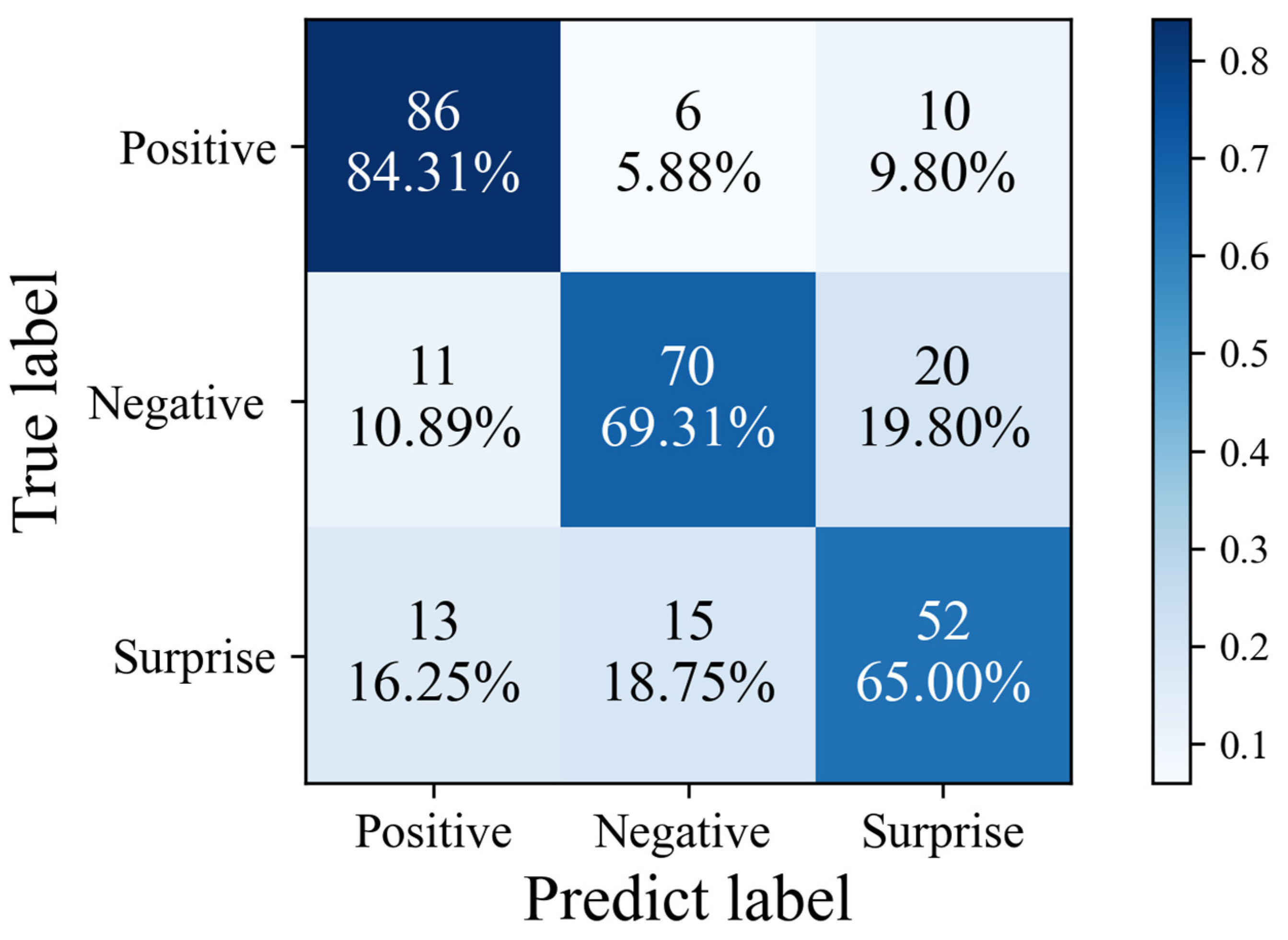
| Method | Positive Emotion Recognition Accuracy (%) | Accuracy of Negative Emotion Recognition (%) | Surprise Recognition Accuracy (%) | Average Recognition Accuracy (%) | Macro-F1 |
|---|---|---|---|---|---|
| C3D [37] | 58.15 | 40.83 | 45.00 | 47.99 | 0.44 |
| R(2 + 1)D- 18 [38] | 61.86 | 49.04 | 48.26 | 53.05 | 0.50 |
| 3D ResNet-18 [39] | 62.67 | 45.87 | 47.35 | 51.96 | 0.49 |
| EC-STFL [40] | 61.06 | 44.68 | 46.15 | 50.63 | 0.50 |
| Resnet-18 + LSTM [41] | 68.03 | 52.13 | 51.24 | 57.13 | 0.53 |
| Resnet-18 + GRU [42] | 66.54 | 54.21 | 52.00 | 57.58 | 0.55 |
| Former-DFER [43] | 67.68 | 54.79 | 56.43 | 59.63 | 0.56 |
| CEFLNet [44] | 67.67 | 51.67 | 52.08 | 57.14 | 0.56 |
| EST [45] | 70.10 | 55.67 | 52.87 | 59.54 | 0.57 |
| STT [46] | 62.14 | 60.09 | 53.20 | 58.47 | 0.56 |
| NR-DFERNet [47] | 73.49 | 58.31 | 62.60 | 64.80 | 0.60 |
| VideoMAE [48] | 75.19 | 58.41 | 63.50 | 65.70 | 0.61 |
| MAE-DFER [49] | 76.02 | 65.70 | 61.25 | 67.65 | 0.62 |
| MADV-Net | 84.31 | 69.31 | 65.00 | 72.87 | 0.69 |
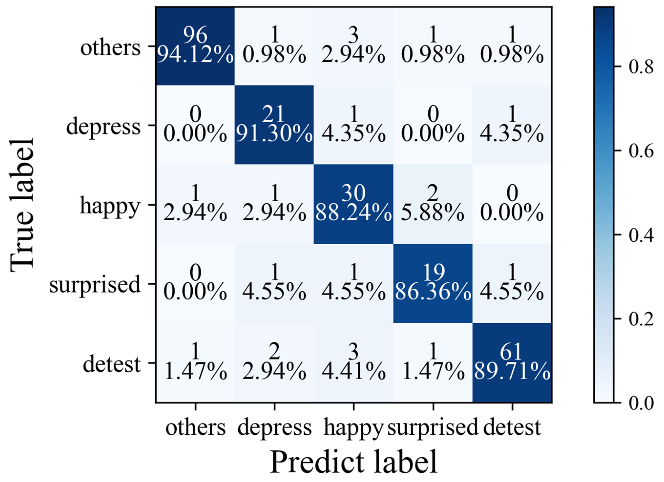
| Method | Happy (%) | Constrain (%) | Surprised (%) | Detest (%) | Other (%) | Average Recognition Accuracy (%) | Macro-F1 |
|---|---|---|---|---|---|---|---|
| C3D [37] | 54.00 | 62.25 | 49.25 | 66.00 | 68.50 | 60.00 | 0.56 |
| R(2 + 1)D- 18 [38] | 62.30 | 66.70 | 58.60 | 67.20 | 68.60 | 64.68 | 0.59 |
| 3D ResNet-18 [39] | 65.00 | 68.00 | 72.00 | 71.50 | 71.50 | 69.60 | 0.61 |
| EC-STFL [40] | 66.25 | 68.68 | 74.00 | 72.50 | 74.00 | 71.08 | 0.68 |
| Resnet-18 + LSTM [41] | 74.00 | 71.50 | 70.50 | 74.20 | 75.20 | 73.08 | 0.69 |
| Resnet-18 + GRU [42] | 74.50 | 76.00 | 74.50 | 74.00 | 70.20 | 73.84 | 0.68 |
| Former-DFER [43] | 78.00 | 78.00 | 77.60 | 75.50 | 77.50 | 77.32 | 0.71 |
| CEFLNet [44] | 79.50 | 81.20 | 80.00 | 81.50 | 84.00 | 81.24 | 0.76 |
| EST [45] | 86.00 | 79.60 | 82.00 | 80.00 | 81.60 | 81.84 | 0.78 |
| STT [46] | 86.50 | 81.25 | 82.45 | 80.60 | 82.00 | 82.56 | 0.79 |
| NR-DFERNet [47] | 86.50 | 85.00 | 86.00 | 84.50 | 82.50 | 84.90 | 0.80 |
| VideoMAE [48] | 87.00 | 88.20 | 79.50 | 85.50 | 85.00 | 85.04 | 0.81 |
| MAE-DFER [49] | 90.00 | 86.50 | 86.00 | 84.00 | 86.00 | 86.50 | 0.82 |
| MADV-Net | 94.12 | 91.30 | 88.24 | 86.36 | 89.71 | 89.94 | 0.84 |
| Method | Happy (%) | Sad (%) | Neutral (%) | Angry (%) | Surprised (%) | Despise (%) | Frightened (%) | Average Recognition Accuracy (%) | Macro-F1 |
|---|---|---|---|---|---|---|---|---|---|
| C3D [37] | 48.20 | 45.53 | 52.71 | 53.72 | 63.45 | 54.93 | 60.23 | 54.11 | 0.52 |
| R(2 + 1)D-18 [38] | 79.65 | 39.02 | 56.65 | 51.02 | 67.25 | 63.25 | 62.08 | 59.84 | 0.55 |
| 3D ResNet-18 [39] | 76.32 | 50.20 | 64.15 | 61.95 | 46.53 | 61.02 | 62.65 | 60.40 | 0.58 |
| EC-STFL [40] | 78.25 | 50.05 | 54.25 | 60.25 | 65.25 | 62.83 | 60.57 | 61.63 | 0.59 |
| Resnet-18 + LSTM [41] | 81.90 | 60.95 | 62.60 | 66.97 | 53.25 | 60.20 | 60.82 | 63.81 | 0.60 |
| Resnet-18 + GRU [42] | 80.65 | 61.50 | 61.45 | 68.51 | 52.02 | 70.89 | 71.54 | 66.65 | 0.62 |
| Former-DFER [43] | 83.58 | 67.58 | 67.00 | 70.00 | 56.25 | 73.54 | 71.57 | 69.93 | 0.64 |
| CEFLNet [44] | 84.24 | 64.56 | 67.01 | 70.03 | 52.00 | 80.00 | 81.00 | 71.26 | 0.66 |
| EST [45] | 86.25 | 65.25 | 67.15 | 72.54 | 78.81 | 65.21 | 79.25 | 73.49 | 0.68 |
| STT [46] | 87.12 | 64.25 | 62.65 | 71.56 | 63.21 | 73.48 | 75.68 | 71.13 | 0.69 |
| NR-DFERNet [47] | 88.15 | 64.25 | 68.95 | 69.58 | 60.51 | 81.56 | 82.15 | 73.59 | 0.70 |
| VideoMAE [48] | 91.25 | 68.15 | 70.52 | 74.02 | 61.56 | 85.61 | 79.65 | 75.82 | 0.71 |
| MAE-DFER [49] | 91.85 | 70.95 | 72.56 | 75.21 | 65.21 | 80.56 | 83.69 | 77.14 | 0.72 |
| MADV-Net | 92.90 | 78.99 | 79.02 | 84.36 | 81.36 | 85.37 | 81.25 | 83.32 | 0.78 |
| Method | Happy (%) | Sad (%) | Detest (%) | Angry (%) | Other (%) | Despise (%) | Frightened (%) | Surprised (%) | Average Recognition Accuracy (%) | Macro-F1 |
|---|---|---|---|---|---|---|---|---|---|---|
| C3D [37] | 65.00 | 57.00 | 58.60 | 60.00 | 62.00 | 61.20 | 68.00 | 61.64 | 61.68 | 0.58 |
| R(2 + 1)D- 18 [38] | 67.50 | 60.00 | 63.20 | 67.00 | 61.00 | 64.00 | 68.50 | 64.40 | 64.45 | 0.59 |
| 3D ResNet-18 [39] | 68.00 | 69.00 | 72.00 | 70.00 | 61.00 | 63.20 | 64.00 | 66.72 | 66.74 | 0.61 |
| EC-STFL [40] | 72.00 | 70.00 | 68.00 | 68.00 | 64.00 | 65.00 | 65.00 | 67.36 | 67.42 | 0.63 |
| Resnet-18 + LSTM [41] | 74.50 | 74.00 | 70.00 | 72.00 | 74.00 | 68.50 | 68.00 | 71.56 | 71.57 | 0.65 |
| Resnet-18 + GRU [42] | 78.00 | 75.00 | 67.50 | 68.00 | 65.00 | 74.00 | 70.00 | 71.06 | 71.07 | 0.66 |
| Former-DFER [43] | 80.00 | 82.00 | 70.00 | 72.00 | 74.00 | 72.00 | 73.00 | 74.68 | 74.71 | 0.68 |
| CEFLNet [44] | 80.00 | 78.00 | 72.00 | 78.00 | 70.00 | 71.00 | 73.50 | 74.62 | 74.64 | 0.69 |
| EST [45] | 82.00 | 82.00 | 85.00 | 81.00 | 75.00 | 74.50 | 76.50 | 79.36 | 79.42 | 0.71 |
| STT [46] | 84.00 | 82.50 | 86.00 | 84.00 | 80.00 | 76.00 | 78.00 | 81.50 | 81.50 | 0.79 |
| NR-DFERNet [47] | 86.00 | 86.00 | 85.00 | 86.00 | 85.00 | 86.00 | 84.00 | 85.36 | 85.42 | 0.81 |
| VideoMAE [48] | 92.00 | 94.00 | 90.00 | 86.00 | 84.00 | 85.00 | 86.00 | 88.12 | 88.14 | 0.82 |
| MAE-DFER [49] | 91.00 | 94.00 | 92.00 | 88.00 | 94.00 | 86.00 | 84.00 | 89.80 | 89.85 | 0.84 |
| MADV-Net | 93.95 | 88.85 | 86.36 | 91.97 | 86.60 | 90.06 | 88.98 | 89.47 | 89.53 | 0.88 |
Disclaimer/Publisher’s Note: The statements, opinions and data contained in all publications are solely those of the individual author(s) and contributor(s) and not of MDPI and/or the editor(s). MDPI and/or the editor(s) disclaim responsibility for any injury to people or property resulting from any ideas, methods, instructions or products referred to in the content. |
© 2025 by the authors. Licensee MDPI, Basel, Switzerland. This article is an open access article distributed under the terms and conditions of the Creative Commons Attribution (CC BY) license (https://creativecommons.org/licenses/by/4.0/).
Share and Cite
Kong, W.; You, Z.; Lv, X. 3D Micro-Expression Recognition Based on Adaptive Dynamic Vision. Sensors 2025, 25, 3175. https://doi.org/10.3390/s25103175
Kong W, You Z, Lv X. 3D Micro-Expression Recognition Based on Adaptive Dynamic Vision. Sensors. 2025; 25(10):3175. https://doi.org/10.3390/s25103175
Chicago/Turabian StyleKong, Weiyi, Zhisheng You, and Xuebin Lv. 2025. "3D Micro-Expression Recognition Based on Adaptive Dynamic Vision" Sensors 25, no. 10: 3175. https://doi.org/10.3390/s25103175
APA StyleKong, W., You, Z., & Lv, X. (2025). 3D Micro-Expression Recognition Based on Adaptive Dynamic Vision. Sensors, 25(10), 3175. https://doi.org/10.3390/s25103175