

Towards Anytime Optical Flow Estimation with Event Cameras

 , , ,
, , , 
Abstract
1. Introduction
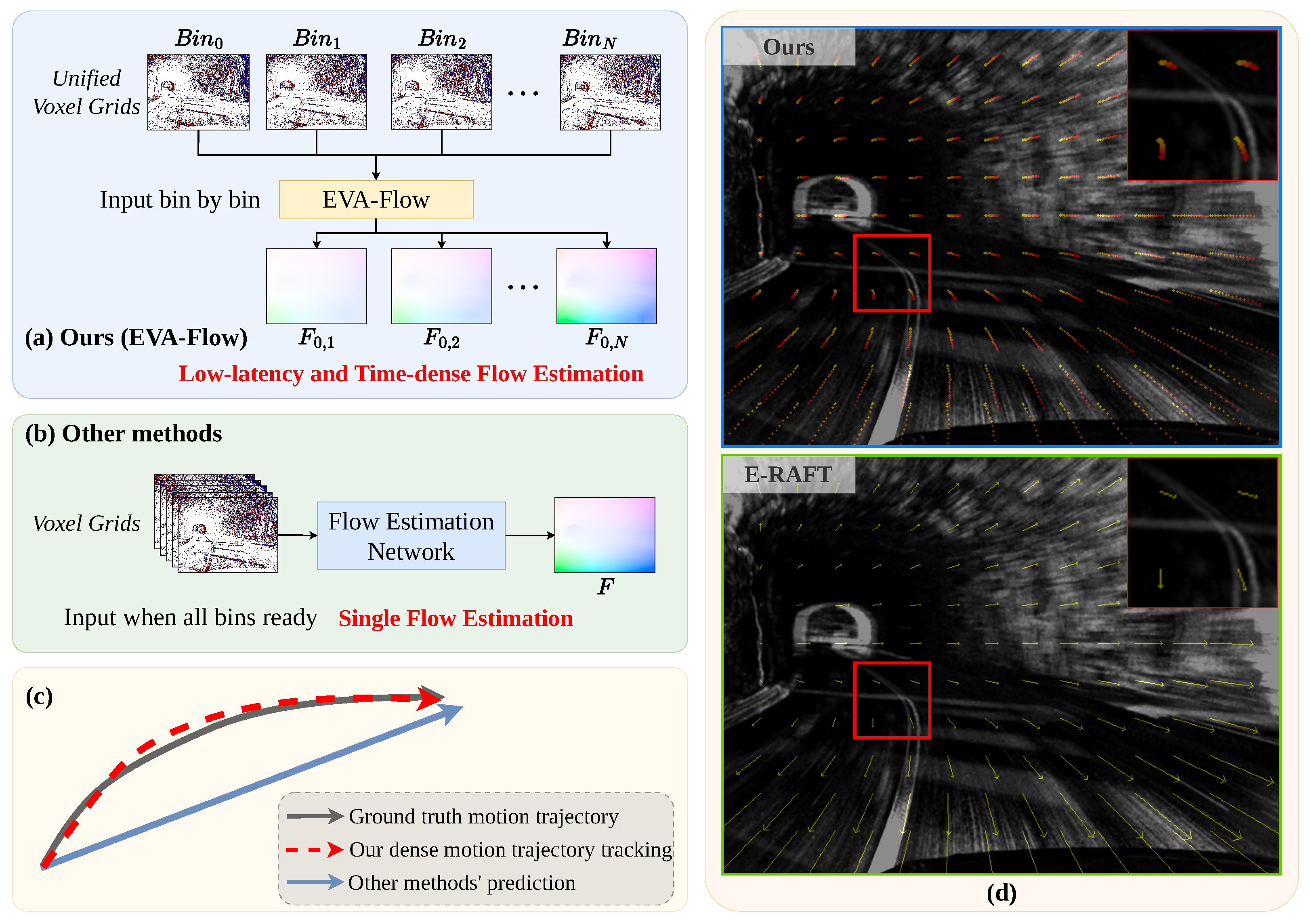
- EVA-Flow Framework: An EVent-based Anytime optical Flow estimation framework that achieves breakthroughs in latency and temporal resolution. The architecture features two novel components: (1) unified voxel grid (UVG) representation enabling ultra-low latency data encoding, and (2) A time-dense feature warping mechanism where shared-weight SMR modules propagate flow predictions across temporal scales. This structural design fundamentally enables single-supervision learning—only final outputs require low-frame-rate supervision while implicitly regularizing intermediate time steps through feature warping recursion.
- Rectified Flow Warp Loss (RFWL): A new unsupervised metric specifically designed for evaluating event-based optical flow precision. This self-consistent measurement provides theoretical guarantees for temporal continuity validation of high-frequency optical flow estimation.
- Systematic Validation: Comprehensive benchmarking demonstrates competitive accuracy, super-low latency, time-dense motion estimation and strong generalization capability. Quantitative analyses using RFWL further confirm the reliability of our continuous-time motion estimation.
2. Related Work
2.1. Optical Flow Estimation
2.2. Event-Based Optical Flow
3. Method
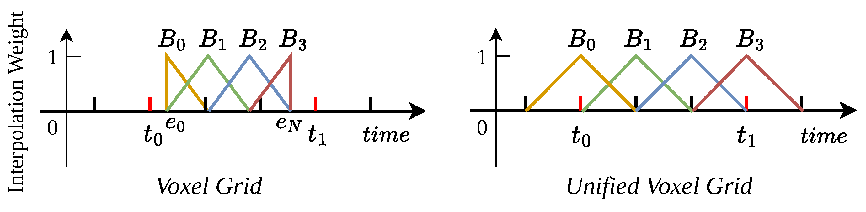
3.1. Event Representation: Unified Voxel Grid
3.2. Event Anytime Flow Estimation Framework
3.3. Supervision
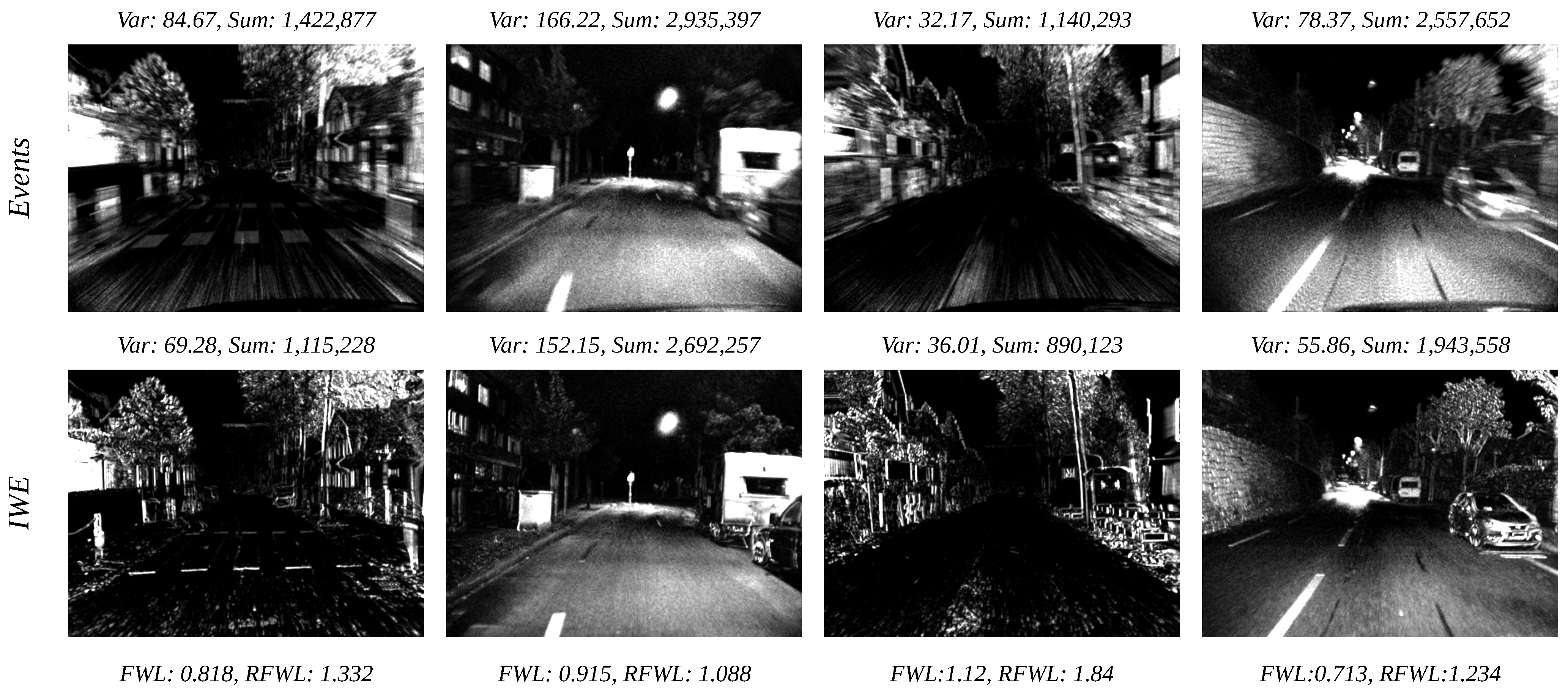
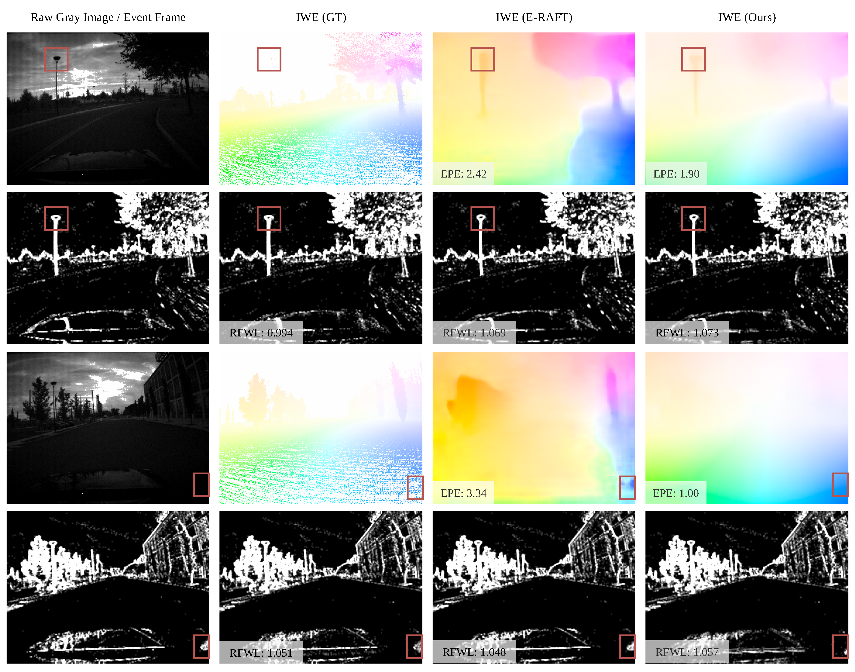
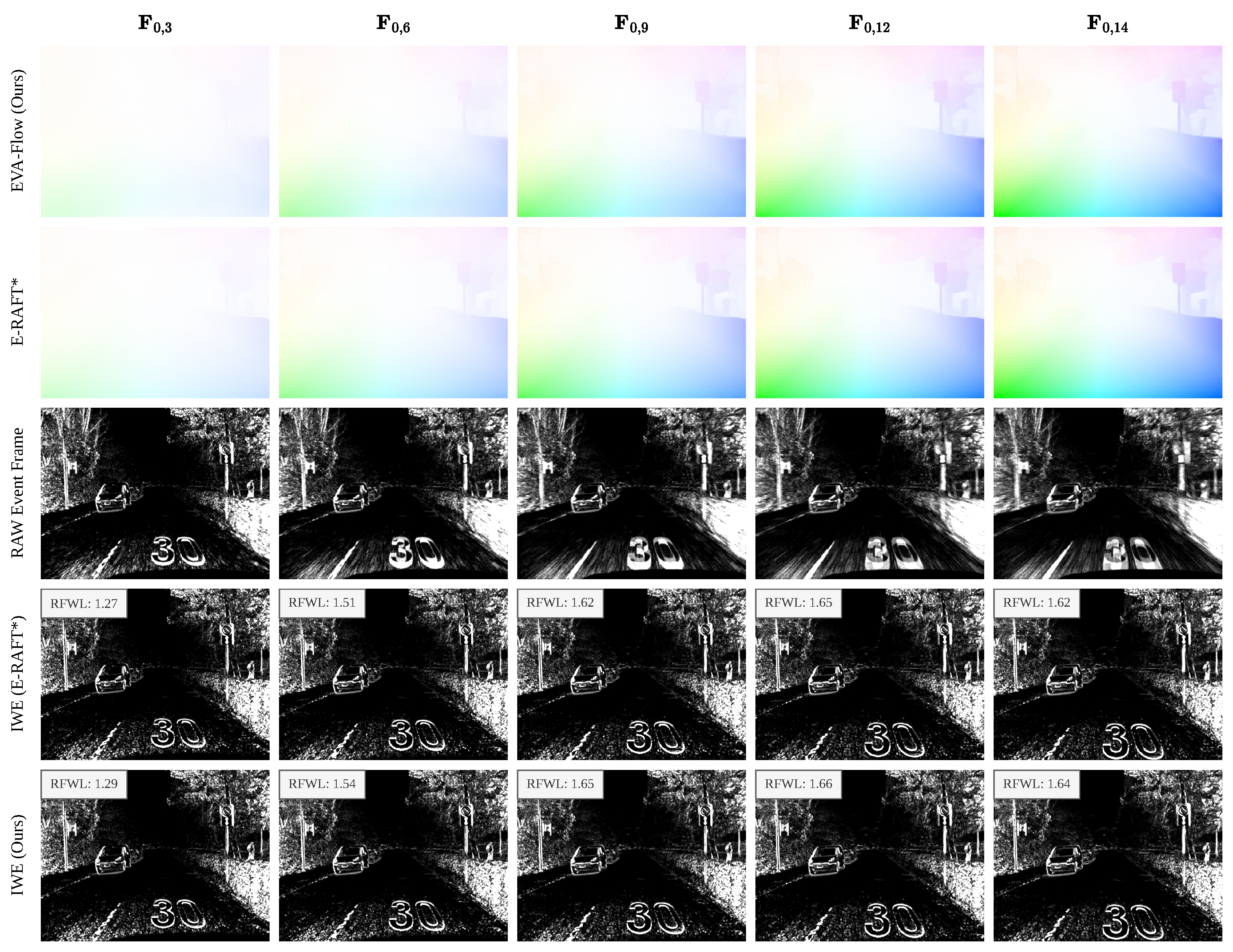
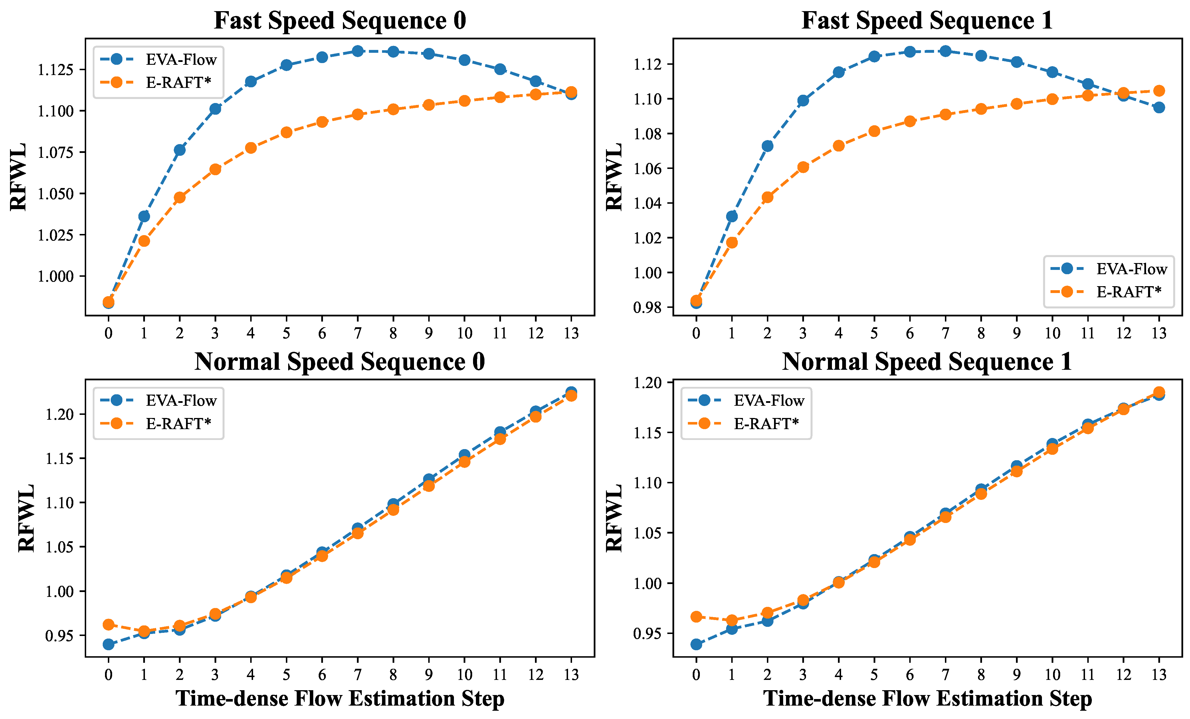
3.4. Rectified Flow Warp Loss
4. Experimental Results
4.1. Datasets
4.2. Implementation Details
4.3. Regular Flow Evaluation Prototype
4.4. Time-Dense Optical Flow Evaluation
4.5. Ablation Study
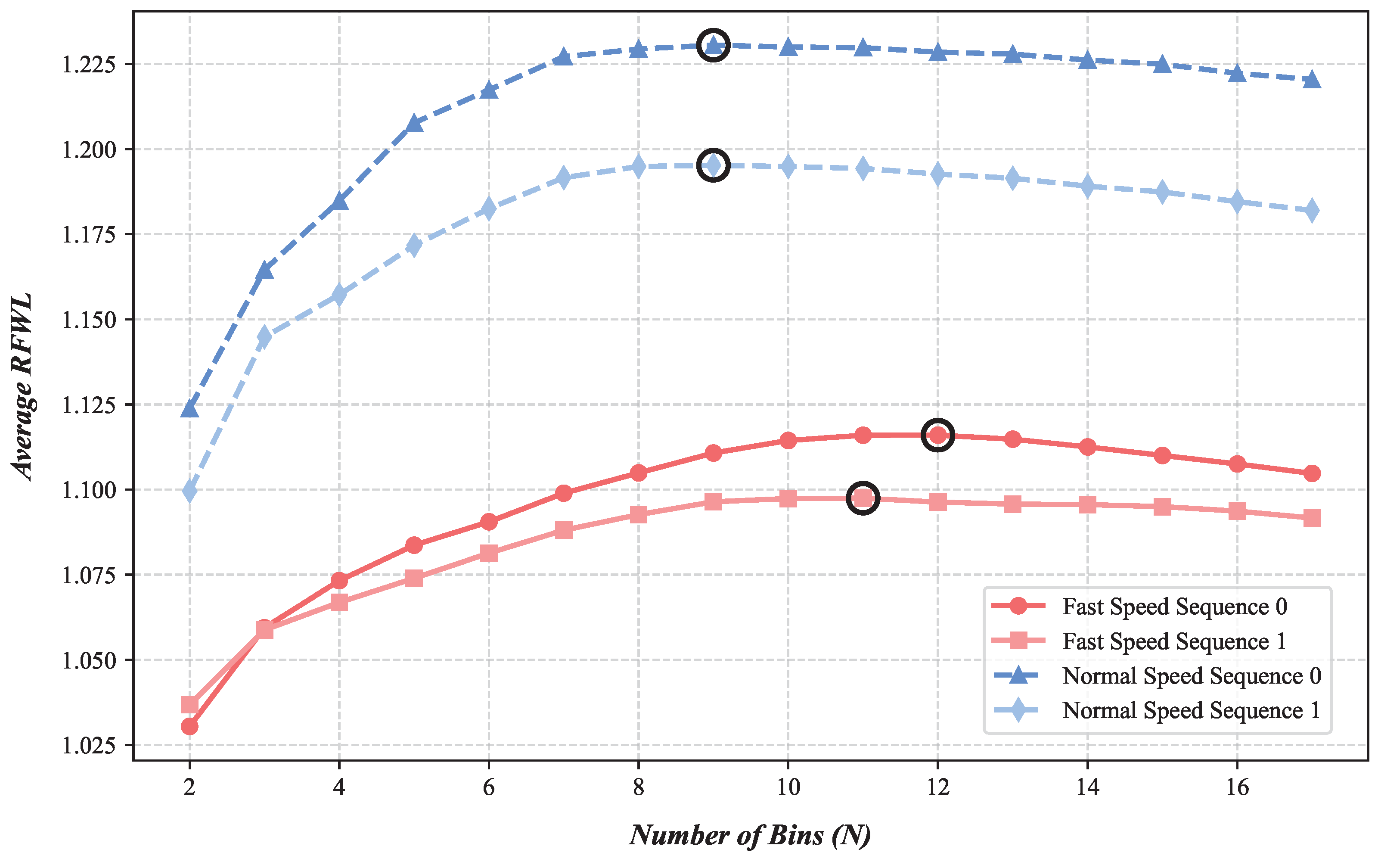
- For high-speed scenarios, using during inference is recommended for optimal time-dense performance.
- For moderate/low-speed or low-light (sparse event) scenarios, using a longer ms during inference is likely beneficial to ensure sufficient event accumulation per bin.
5. Limitations and Future Work
- Accuracy Relative to Non-Time-Dense Methods: Although competitive, EVA-Flow’s final prediction accuracy (e.g., EPE) is slightly lower than some state-of-the-art non-time-dense methods that utilize computationally intensive correlation volumes and focus solely on maximizing accuracy between two distant time points. Our current SMR module relies on implicit warp alignment for efficiency and time-density. Future work could explore hybrid approaches, potentially incorporating lightweight correlation features or attention mechanisms to enhance accuracy, especially for complex motions, without drastically increasing latency or computational cost.
- Sparse Temporal Supervision: EVA-Flow achieves time-dense prediction but is still primarily supervised using ground-truth optical flow provided at a much lower frame rate (e.g., 10 Hz on DSEC). While our unsupervised RFWL metric helps validate intermediate flows, the network lacks direct, dense temporal supervision during training. Developing techniques for generating reliable time-continuous ground truth, perhaps through advanced interpolation or simulation, or exploring unsupervised/self-supervised learning objectives specifically designed for time-dense event flow could further enhance intermediate flow accuracy and reliability.
- Event-Only Input: The current EVA-Flow framework operates solely on event data. While this highlights the richness of information within event streams, incorporating asynchronous image frames from the event camera (like Davis sensors) could provide complementary information, particularly in static scenes, low-texture areas, or during periods of low event activity. Designing efficient multi-modal fusion architectures that leverage both event dynamics and frame appearance is a promising direction for improving robustness and overall accuracy.
6. Conclusions
Author Contributions
Funding
Institutional Review Board Statement
Informed Consent Statement
Data Availability Statement
Acknowledgments
Conflicts of Interest
References
- Gallego, G.; Delbruck, T.; Orchard, G.; Bartolozzi, C.; Taba, B.; Censi, A.; Leutenegger, S.; Davison, A.; Conradt, J.; Daniilidis, K.; et al. Event-based vision: A survey. IEEE Trans. Pattern Anal. Mach. Intell. 2022, 44, 154–180. [Google Scholar] [CrossRef] [PubMed]
- Zhu, A.Z.; Yuan, L.; Chaney, K.; Daniilidis, K. EV-FlowNet: Self-supervised optical flow estimation for event-based cameras. In Proceedings of the Robotics: Science and Systems (RSS), Pittsburgh, PA, USA, 26–30 June 2018. [Google Scholar] [CrossRef]
- Gehrig, M.; Millhäusler, M.; Gehrig, D.; Scaramuzza, D. E-RAFT: Dense optical flow from event cameras. In Proceedings of the 2021 International Conference on 3D Vision (3DV), London, UK, 1–3 December 2021; pp. 197–206. [Google Scholar]
- Zhang, J.; Yang, K.; Stiefelhagen, R. ISSAFE: Improving semantic segmentation in accidents by fusing event-based data. In Proceedings of the 2021 IEEE/RSJ International Conference on Intelligent Robots and Systems (IROS), Prague, Czech Republic, 27 September–1 October 2021; pp. 1132–1139. [Google Scholar]
- Zhang, J.; Yang, K.; Stiefelhagen, R. Exploring event-driven dynamic context for accident scene segmentation. IEEE Trans. Intell. Transp. Syst. 2022, 23, 2606–2622. [Google Scholar] [CrossRef]
- Zhou, H.; Chang, Y.; Liu, H.; Yan, W.; Duan, Y.; Shi, Z.; Yan, L. Exploring the Common Appearance-Boundary Adaptation for Nighttime Optical Flow. arXiv 2024, arXiv:2401.17642. [Google Scholar]
- Zhu, A.Z.; Yuan, L.; Chaney, K.; Daniilidis, K. Unsupervised event-based learning of optical flow, depth, and egomotion. In Proceedings of the 2019 IEEE/CVF Conference on Computer Vision and Pattern Recognition (CVPR), Long Beach, CA, USA, 15–20 June 2019; pp. 989–997. [Google Scholar]
- Zhu, A.Z.; Thakur, D.; Özaslan, T.; Pfrommer, B.; Kumar, V.; Daniilidis, K. The multivehicle stereo event camera dataset: An event camera dataset for 3D perception. IEEE Robot. Autom. Lett. 2018, 3, 2032–2039. [Google Scholar] [CrossRef]
- Gehrig, M.; Aarents, W.; Gehrig, D.; Scaramuzza, D. DSEC: A stereo event camera dataset for driving scenarios. IEEE Robot. Autom. Lett. 2021, 6, 4947–4954. [Google Scholar] [CrossRef]
- Dosovitskiy, A.; Fischer, P.; Ilg, E.; Hausser, P.; Hazirbas, C.; Golkov, V.; van der Smagt, P.; Cremers, D.; Brox, T. FlowNet: Learning optical flow with convolutional networks. In Proceedings of the 2015 IEEE/CVF International Conference on Computer Vision (ICCV), Santiago, Chile, 7–13 December 2015; IEEE: Piscataway, NJ, USA, 2015; pp. 2758–2766. [Google Scholar]
- Ilg, E.; Mayer, N.; Saikia, T.; Keuper, M.; Dosovitskiy, A.; Brox, T. FlowNet 2.0: Evolution of optical flow estimation with deep networks. In Proceedings of the 2017 IEEE/CVF Conference on Computer Vision and Pattern Recognition (CVPR), Honolulu, HI, USA, 21–26 July 2017; IEEE: Piscataway, NJ, USA, 2017; pp. 1647–1655. [Google Scholar]
- Hui, T.W.; Tang, X.; Loy, C.C. LiteFlowNet: A lightweight convolutional neural network for optical flow estimation. In Proceedings of the 2018 IEEE/CVF Conference on Computer Vision and Pattern Recognition (CVPR), Salt Lake City, UT, USA, 18–23 June 2018; IEEE: Piscataway, NJ, USA, 2018; pp. 8981–8989. [Google Scholar]
- Hui, T.W.; Tang, X.; Loy, C.C. A lightweight optical flow CNN—Revisiting data fidelity and regularization. IEEE Trans. Pattern Anal. Mach. Intell. 2021, 43, 2555–2569. [Google Scholar] [CrossRef] [PubMed]
- Ranjan, A.; Black, M.J. Optical flow estimation using a spatial pyramid network. In Proceedings of the 2017 IEEE/CVF Conference on Computer Vision and Pattern Recognition (CVPR), Honolulu, HI, USA, 21–26 July 2017; IEEE: Piscataway, NJ, USA, 2017; pp. 2720–2729. [Google Scholar]
- Sun, D.; Yang, X.; Liu, M.Y.; Kautz, J. PWC-net: CNNs for optical flow using pyramid, warping, and cost volume. In Proceedings of the 2018 IEEE/CVF Conference on Computer Vision and Pattern Recognition (CVPR), Salt Lake City, UT, USA, 18–23 June 2018; pp. 8934–8943. [Google Scholar]
- Teed, Z.; Deng, J. RAFT: Recurrent all-pairs field transforms for optical flow. In Proceedings of the European Conference on Computer Vision (ECCV), Seattle, WA, USA, 14–19 June 2020; Volume 12347, pp. 402–419. [Google Scholar]
- Shi, H.; Zhou, Y.; Yang, K.; Yin, X.; Wang, K. CSFlow: Learning optical flow via cross strip correlation for autonomous driving. In Proceedings of the 2022 IEEE Intelligent Vehicles Symposium (IV), Aachen, Germany, 5–9 June 2022; pp. 1851–1858. [Google Scholar]
- Huang, Z.; Shi, X.; Zhang, C.; Wang, Q.; Cheung, K.C.; Qin, H.; Dai, J.; Li, H. FlowFormer: A transformer architecture for optical flow. In Proceedings of the European Conference on Computer Vision (ECCV), Tel Aviv, Israel, 23–27 October 2022; Volume 13677, pp. 668–685. [Google Scholar]
- Benosman, R.; Clercq, C.; Lagorce, X.; Ieng, S.H.; Bartolozzi, C. Event-based visual flow. IEEE Trans. Neural Netw. Learn. Syst. 2014, 25, 407–417. [Google Scholar] [CrossRef] [PubMed]
- Mueggler, E.; Forster, C.; Baumli, N.; Gallego, G.; Scaramuzza, D. Lifetime Estimation of Events from Dynamic Vision Sensors. In Proceedings of the 2015 IEEE International Conference on Robotics and Automation (ICRA), Seattle, WA, USA, 26–30 May 2015; IEEE: Piscataway, NJ, USA, 2015; pp. 4874–4881. [Google Scholar]
- Low, W.F.; Gao, Z.; Xiang, C.; Ramesh, B. SOFEA: A non-iterative and robust optical flow estimation algorithm for dynamic vision sensors. In Proceedings of the IEEE/CVF Conference on Computer Vision and Pattern Recognition Workshops (CVPRW), Seattle, WA, USA, 14–19 June 2020; pp. 368–377. [Google Scholar]
- Gallego, G.; Rebecq, H.; Scaramuzza, D. A unifying contrast maximization framework for event cameras, with applications to motion, depth, and optical flow estimation. In Proceedings of the 2018 IEEE/CVF Conference on Computer Vision and Pattern Recognition (CVPR), Salt Lake City, UT, USA, 18–23 June 2018; IEEE: Piscataway, NJ, USA, 2018; pp. 3867–3876. [Google Scholar]
- Shiba, S.; Aoki, Y.; Gallego, G. Secrets of event-based optical flow. In Proceedings of the European Conference on Computer Vision (ECCV), Tel Aviv, Israel, 23–27 October 2022; Volume 13678, pp. 628–645. [Google Scholar]
- Shiba, S.; Klose, Y.; Aoki, Y.; Gallego, G. Secrets of Event-based Optical Flow, Depth and Ego-motion Estimation by Contrast Maximization. IEEE Trans. Pattern Anal. Mach. Intell. 2024, 46, 7742–7759. [Google Scholar] [CrossRef] [PubMed]
- Almatrafi, M.; Baldwin, R.; Aizawa, K.; Hirakawa, K. Distance surface for event-based optical flow. IEEE Trans. Pattern Anal. Mach. Intell. 2020, 42, 1547–1556. [Google Scholar] [CrossRef] [PubMed]
- Delbruck, T. Frame-free dynamic digital vision. In Proceedings of the International Symposium on Secure-Life Electronics Advanced Electronics for Quality Life and Society, Tokyo, Japan, 6–7 March 2008; Volume 1, pp. 21–26. [Google Scholar]
- Ye, C.; Mitrokhin, A.; Fermüller, C.; Yorke, J.A.; Aloimonos, Y. Unsupervised learning of dense optical flow, depth and egomotion with event-based sensors. In Proceedings of the 2020 IEEE/RSJ International Conference on Intelligent Robots and Systems (IROS), Las Vegas, NV, USA, 25–29 October 2020; pp. 5831–5838. [Google Scholar]
- Sun, H.; Dao, M.Q.; Fremont, V. 3D-FlowNet: Event-based optical flow estimation with 3D representation. In Proceedings of the 2022 IEEE Intelligent Vehicles Symposium (IV), Aachen, Germany, 5–9 June 2022; pp. 1845–1850. [Google Scholar]
- Hu, L.; Zhao, R.; Ding, Z.; Ma, L.; Shi, B.; Xiong, R.; Huang, T. Optical flow estimation for spiking camera. In Proceedings of the 2022 IEEE/CVF Conference on Computer Vision and Pattern Recognition (CVPR), New Orleans, LA, USA, 19–20 June 2022; IEEE: Piscataway, NJ, USA, 2022; pp. 17823–17832. [Google Scholar]
- Lee, C.; Kosta, A.K.; Zhu, A.Z.; Chaney, K.; Daniilidis, K.; Roy, K. Spike-flownet: Event-based optical flow estimation with energy-efficient hybrid neural networks. In Proceedings of the European Conference on Computer Vision, Glasgow, UK, 23–28 August 2020; Springer: Berlin/Heidelberg, Germany, 2020; pp. 366–382. [Google Scholar]
- Li, Y.; Huang, Z.; Chen, S.; Shi, X.; Li, H.; Bao, H.; Cui, Z.; Zhang, G. Blinkflow: A dataset to push the limits of event-based optical flow estimation. In Proceedings of the 2023 IEEE/RSJ International Conference on Intelligent Robots and Systems (IROS), Detroit, MI, USA, 1–5 October 2023; IEEE: Piscataway, NJ, USA, 2023; pp. 3881–3888. [Google Scholar]
- Vaswani, A.; Shazeer, N.; Parmar, N.; Uszkoreit, J.; Jones, L.; Gomez, A.N.; Kaiser, L.; Polosukhin, I. Attention is all you need. In Proceedings of the 31st Conference on Neural Information Processing Systems (NeurIPS 2017), Long Beach, CA, USA, 4–9 December 2017. [Google Scholar]
- Liu, H.; Chen, G.; Qu, S.; Zhang, Y.; Li, Z.; Knoll, A.; Jiang, C. TMA: Temporal motion aggregation for event-based optical flow. In Proceedings of the IEEE/CVF International Conference on Computer Vision, Paris, France, 2–6 October 2023; pp. 9685–9694. [Google Scholar]
- Wu, Y.; Paredes-Vallés, F.; De Croon, G.C. Lightweight event-based optical flow estimation via iterative deblurring. In Proceedings of the 2024 IEEE International Conference on Robotics and Automation (ICRA), IEEE, Yokohama, Japan, 13–17 May 2024; pp. 14708–14715. [Google Scholar]
- Chaney, K.; Panagopoulou, A.; Lee, C.; Roy, K.; Daniilidis, K. Self-supervised optical flow with spiking neural networks and event based cameras. In Proceedings of the 2021 IEEE/RSJ International Conference on Intelligent Robots and Systems (IROS), Prague, Czech Republic, 27 September–1 October 2021; pp. 5892–5899. [Google Scholar]
- Paredes-Vallés, F.; Scheper, K.Y.; De Wagter, C.; De Croon, G.C. Taming contrast maximization for learning sequential, low-latency, event-based optical flow. In Proceedings of the IEEE/CVF International Conference on Computer Vision, Paris, France, 2–6 October 2023; pp. 9695–9705. [Google Scholar]
- Wan, Z.; Dai, Y.; Mao, Y. Learning Dense and Continuous Optical Flow From an Event Camera. IEEE Trans. Image Process. 2022, 31, 7237–7251. [Google Scholar] [CrossRef] [PubMed]
- Ponghiran, W.; Liyanagedera, C.M.; Roy, K. Event-based temporally dense optical flow estimation with sequential learning. In Proceedings of the 2023 IEEE/CVF International Conference on Computer Vision (ICCV), Paris, France, 2–6 October 2023; IEEE: Piscataway, NJ, USA, 2023; pp. 9827–9836. [Google Scholar]
- Gehrig, M.; Muglikar, M.; Scaramuzza, D. Dense continuous-time optical flow from event cameras. IEEE Trans. Pattern Anal. Mach. Intell. 2024, 46, 4736–4746. [Google Scholar] [CrossRef] [PubMed]
- Baldwin, R.W.; Liu, R.; Almatrafi, M.; Asari, V.; Hirakawa, K. Time-ordered recent event (TORE) volumes for event cameras. IEEE Trans. Pattern Anal. Mach. Intell. 2023, 45, 2519–2532. [Google Scholar] [CrossRef] [PubMed]
- Gehrig, D.; Loquercio, A.; Derpanis, K.G.; Scaramuzza, D. End-to-end learning of representations for asynchronous event-based data. In Proceedings of the 2019 IEEE/CVF International Conference on Computer Vision (ICCV), Seoul, Republic of Korea, 27 October–2 November 2019; IEEE: Piscataway, NJ, USA, 2019; pp. 5633–5643. [Google Scholar]
- Ballas, N.; Yao, L.; Pal, C.; Courville, A. Delving deeper into convolutional networks for learning video representations. arXiv 2015, arXiv:1511.06432. [Google Scholar]
- Stoffregen, T.; Scheerlinck, C.; Scaramuzza, D.; Drummond, T.; Barnes, N.; Kleeman, L.; Mahony, R. Reducing the sim-to-real gap for event cameras. In Proceedings of the European Conference on Computer Vision (ECCV), Seattle, WA, USA, 14–19 June 2020; Volume 12372, pp. 534–549. [Google Scholar]
- Ding, Z.; Zhao, R.; Zhang, J.; Gao, T.; Xiong, R.; Yu, Z.; Huang, T. Spatio-temporal recurrent networks for event-based optical flow estimation. In Proceedings of the AAAI conference on Artificial Intelligence, Vancouver, BC, Canada, 28 February–1 March 2022; Volume 36, pp. 525–533. [Google Scholar]
- Hagenaars, J.; Paredes-Vallés, F.; De Croon, G. Self-supervised learning of event-based optical flow with spiking neural networks. In Proceedings of the Advances in Neural Information Processing Systems (NeurIPS), Virtual, 6–14 December 2021; Volume 34, pp. 7167–7179. [Google Scholar]


| Method | Params | GMACs | Latency | Prediction Rate | Supervision | EPE | AE | 1PE | 3PE |
|---|---|---|---|---|---|---|---|---|---|
| EV-FlowNet [2] | 14 M | 62 | 100 ms | 10 Hz | Self Supervised | 2.32 | 7.90 | 55.4 | 18.6 |
| E-RFAT [3] | 5.3 M | 41 | 100 ms | 10 Hz | 10 Hz GT | 0.79 | 2.85 | 12.7 | 2.7 |
| IDNet 1iter [34] | 1.4 M | 55 | 7.14 ms | 10 Hz | 10 Hz GT | 1.30 | 4.82 | 33.7 | 6.7 |
| TIDNet [34] | 1.9 M | 55 | 7.14 ms | 10 Hz | 10 Hz GT | 0.84 | 3.41 | 14.7 | 2.8 |
| TMA [33] | 6.9 M | 56 | 100 ms | 10 Hz | 10 Hz GT | 0.74 | - | 10.9 | 2.3 |
| BFlow [39] | 5.6 M | 379 | 100 ms | Bézier Curve | 10 Hz GT | 0.75 | 2.68 | 11.9 | 2.44 |
| Taming_CM [36] | - | - | 10 ms | 100 Hz | Self Supervised | 2.33 | 10.56 | 68.3 | 17.8 |
| LSTM-FlowNet [38] | 53.6 M | 444 | 10 ms | 100 Hz | 100 Hz GT | 1.28 | - | 47.0 | 6.0 |
| EVA-Flow (ours) | 5.0 M | 16.8 | 5 ms | 200 Hz | 10 Hz GT | 0.88 | 3.31 | 15.9 | 3.2 |
| = 1 | = 4 | ||||
|---|---|---|---|---|---|
| EPE ↓ | Outlier% ↓ | EPE ↓ | Outlier% ↓ | ||
| SSL | EV-FlowNet [2] | 0.49 | 0.20 | 1.23 | 7.30 |
| Spike-FlowNet [30] | 0.49 | - | 1.09 | - | |
| STE-FlowNet [44] | 0.42 | 0.00 | 0.99 | 3.90 | |
| Taming_CM [36] | 0.27 | 0.05 | - | - | |
| USL | Hagenaars et al. [45] | 0.47 | 0.25 | 1.69 | 12.5 |
| Zhu et al. [7] | 0.32 | 0.00 | 1.30 | 9.70 | |
| Shiba et al. [23] | 0.30 | 0.10 | 1.25 | 9.21 | |
| SL | TMA [33] | 0.25 | 0.07 | 0.7 | 1.08 |
| E-RAFT [3] | 0.24 | 0.00 | 0.72 | 1.12 | |
| EVA-Flow (Ours) | 0.25 | 0.00 | 0.82 | 2.41 | |
| E-RAFT [3] (Zero-Shot) | 0.53 | 1.42 | 1.93 | 17.7 | |
| EVA-Flow (Zero-Shot) | 0.39 | 0.07 | 0.96 | 4.92 | |
| Sequence | Method | RFWL | Avg. | |||||||||||||
|---|---|---|---|---|---|---|---|---|---|---|---|---|---|---|---|---|
| thun_01_a | E-RAFT* | 1.039 | 1.104 | 1.163 | 1.211 | 1.250 | 1.282 | 1.309 | 1.333 | 1.355 | 1.374 | 1.392 | 1.407 | 1.422 | 1.434 | 1.291 |
| EVA-Flow (Ours) | 1.030 | 1.101 | 1.166 | 1.217 | 1.256 | 1.289 | 1.316 | 1.339 | 1.359 | 1.379 | 1.394 | 1.408 | 1.421 | 1.434 | 1.294 | |
| thun_01_b | E-RAFT* | 1.058 | 1.134 | 1.193 | 1.236 | 1.277 | 1.313 | 1.349 | 1.382 | 1.416 | 1.447 | 1.476 | 1.500 | 1.522 | 1.539 | 1.346 |
| EVA-Flow (Ours) | 1.046 | 1.135 | 1.208 | 1.262 | 1.305 | 1.340 | 1.370 | 1.393 | 1.419 | 1.444 | 1.467 | 1.490 | 1.512 | 1.532 | 1.352 | |
| interlaken_01_a | E-RAFT* | 1.098 | 1.218 | 1.316 | 1.406 | 1.483 | 1.552 | 1.624 | 1.694 | 1.758 | 1.816 | 1.868 | 1.911 | 1.947 | 1.970 | 1.619 |
| EVA-Flow (Ours) | 1.084 | 1.218 | 1.332 | 1.437 | 1.519 | 1.585 | 1.645 | 1.705 | 1.758 | 1.810 | 1.857 | 1.898 | 1.934 | 1.961 | 1.625 | |
| interlaken_00_b | E-RAFT* | 1.105 | 1.233 | 1.338 | 1.426 | 1.500 | 1.565 | 1.621 | 1.670 | 1.714 | 1.753 | 1.788 | 1.819 | 1.843 | 1.860 | 1.588 |
| EVA-Flow (Ours) | 1.088 | 1.229 | 1.340 | 1.437 | 1.515 | 1.576 | 1.626 | 1.670 | 1.709 | 1.742 | 1.770 | 1.796 | 1.816 | 1.837 | 1.582 | |
| zurich_city_12_a | E-RAFT* | 1.005 | 1.020 | 1.034 | 1.050 | 1.065 | 1.079 | 1.090 | 1.103 | 1.116 | 1.127 | 1.139 | 1.149 | 1.161 | 1.169 | 1.093 |
| EVA-Flow (Ours) | 1.004 | 1.021 | 1.032 | 1.046 | 1.060 | 1.075 | 1.085 | 1.099 | 1.111 | 1.122 | 1.134 | 1.145 | 1.157 | 1.166 | 1.090 | |
| zurich_city_14_c | E-RAFT* | 1.057 | 1.155 | 1.250 | 1.329 | 1.391 | 1.453 | 1.510 | 1.555 | 1.598 | 1.636 | 1.666 | 1.695 | 1.724 | 1.752 | 1.484 |
| EVA-Flow (Ours) | 1.044 | 1.152 | 1.249 | 1.333 | 1.394 | 1.460 | 1.517 | 1.561 | 1.605 | 1.645 | 1.675 | 1.704 | 1.732 | 1.761 | 1.488 | |
| zurich_city_15_a | E-RAFT* | 1.071 | 1.174 | 1.256 | 1.324 | 1.384 | 1.436 | 1.480 | 1.522 | 1.566 | 1.606 | 1.642 | 1.676 | 1.703 | 1.721 | 1.469 |
| EVA-Flow (Ours) | 1.062 | 1.177 | 1.270 | 1.345 | 1.409 | 1.461 | 1.502 | 1.542 | 1.580 | 1.614 | 1.646 | 1.677 | 1.701 | 1.720 | 1.479 | |
| Model | #Bins (Training) | Test Sequences of 10 Hz | #Bins (Evaluating) | Validation Split of 5 Hz | ||||||
|---|---|---|---|---|---|---|---|---|---|---|
| EPE ↓ | AE ↓ | 1PE ↓ | 3PE ↓ | EPE ↓ | 1PE ↓ | 3PE ↓ | 5PE ↓ | |||
| E-RAFT | 15 | 0.79 | 2.85 | 12.7 | 2.7 | 15 | 2.96 | 43.5 | 17.6 | 10.3 |
| EVA-Flow | 6 | 0.955 | 3.29 | 16.7 | 3.9 | 11 | 1.73 | 42.9 | 14.7 | 7.9 |
| 11 | 0.926 | 3.34 | 16.1 | 3.5 | 21 | 1.86 | 51.1 | 15.8 | 8.0 | |
| 15 | 0.895 | 3.39 | 16.1 | 3.3 | 29 | 1.82 | 49.4 | 15.6 | 8.0 | |
| 21 | 0.877 | 3.31 | 15.9 | 3.2 | 41 | 1.89 | 48.7 | 16.8 | 8.8 | |
| 31 | 0.901 | 3.37 | 17.0 | 3.2 | 61 | 2.02 | 53.5 | 18.2 | 9.4 | |
| Event Representation | AE ↓ | EPE ↓ | 1PE ↓ | 3PE ↓ |
|---|---|---|---|---|
| Voxel Grid [7] | 3.48 | 0.96 | 17.7 | 3.65 |
| Unified Voxel Grid | 3.39 | 0.89 | 16.1 | 3.30 |
Disclaimer/Publisher’s Note: The statements, opinions and data contained in all publications are solely those of the individual author(s) and contributor(s) and not of MDPI and/or the editor(s). MDPI and/or the editor(s) disclaim responsibility for any injury to people or property resulting from any ideas, methods, instructions or products referred to in the content. |
© 2025 by the authors. Licensee MDPI, Basel, Switzerland. This article is an open access article distributed under the terms and conditions of the Creative Commons Attribution (CC BY) license (https://creativecommons.org/licenses/by/4.0/).
Share and Cite
Ye, Y.; Shi, H.; Yang, K.; Wang, Z.; Yin, X.; Sun, L.; Wang, Y.; Wang, K. Towards Anytime Optical Flow Estimation with Event Cameras. Sensors 2025, 25, 3158. https://doi.org/10.3390/s25103158
Ye Y, Shi H, Yang K, Wang Z, Yin X, Sun L, Wang Y, Wang K. Towards Anytime Optical Flow Estimation with Event Cameras. Sensors. 2025; 25(10):3158. https://doi.org/10.3390/s25103158
Chicago/Turabian StyleYe, Yaozu, Hao Shi, Kailun Yang, Ze Wang, Xiaoting Yin, Lei Sun, Yaonan Wang, and Kaiwei Wang. 2025. "Towards Anytime Optical Flow Estimation with Event Cameras" Sensors 25, no. 10: 3158. https://doi.org/10.3390/s25103158
APA StyleYe, Y., Shi, H., Yang, K., Wang, Z., Yin, X., Sun, L., Wang, Y., & Wang, K. (2025). Towards Anytime Optical Flow Estimation with Event Cameras. Sensors, 25(10), 3158. https://doi.org/10.3390/s25103158