1. Introduction
Evidence theory has been significantly advanced in multi-source data integration in recent years [
1,
2]. As the cornerstone of the Dempster–Shafer (D-S) theory, the combination rule has been established as the fundamental mechanism in foundational evidence theory. Despite its robust evidence fusion capabilities, the emergence of counter-intuitive outcomes under conflicting evidence conditions has been widely documented [
3,
4]. The foundational breakthrough emerged with Yang and Singh’s [
5] formulation of normalized evidence weighting, which was subsequently refined by Yang and Xu [
6] through the ER Algorithm (ERA) specifically designed to resolve counter-intuitive outcomes in conflicting evidence scenarios.
Building upon the ERA framework, the ER rule [
7] has been developed to extend both Dempster–Shafer evidential theory [
8] and reasoning methodologies [
9]. The ER rule operationalizes evidence synthesis through a generalized probabilistic reasoning framework. This dual-parameter integration systematically combines evidential weight with evidential reliability within a unified probabilistic framework. Evidential weight is determined by relative importance evaluation guided by decision-maker preferences to characterize subjective uncertainty. In parallel, evidential reliability is defined as the evidence source’s capacity for accurate measurement, serving as an objective uncertainty metric. Through orthogonal parameter treatment, reliability and weight are conjunctively embedded in belief distribution modeling. For fuzzy semantic inputs, affiliation functions are systematically applied for uncertainty-preserving information transformation. This synthesis establishes the ER rule as a comprehensive methodology for uncertainty quantification, fuzzy information processing, and probabilistic inference.
Since its introduction, the ER rule has been extensively studied due to its demonstrated scalability and adaptability. The power set domains ER (PSA_ER) framework was enhanced by Wang et al. [
10] through attribute-based evidence integration, while the FoD framework was extended to PSA_ER. Mathematical formulations for dependability and evidence weight were established, along with physical interpretations of model parameters. Parameter optimization was subsequently performed using intelligent optimization techniques to enhance PSA_ER’s performance. A novel ER rule was developed by Du et al. [
11] to address weight–reliability interdependencies, where evidence was recursively combined through orthogonal sum operations with formal theorems and inferences being established. Verification was conducted through numerical comparisons and case studies demonstrating the proposed methods’ effectiveness. ERr-CR was proposed by Wang et al. [
12] for continuous reliability distributions, where reliability was defined as a random variable with probability distributions for paired evidence sources. Expected utility theory was introduced to characterize ERr-CR outputs. The framework was extended to multi-evidence systems, while an ER rule considering multi-source parameter uncertainties was formulated by Wang et al. [
13]. A unified inference model was developed based on ER rule principles.
Meanwhile, ER has been extensively implemented in engineering domains including performance evaluation [
14], pattern classification [
15], and especially in the field of fault diagnosis. Based on ER rules, a new concurrent fault diagnosis model is proposed by Ning et al. [
16]. Multiple sub-ER models are built, forming parallel diagnostic patterns, and thus system reliability is improved. An ER-based time–space domain cascade fusion model (TS-ER for short) is proposed by Xu et al. [
17] for rudder fault diagnosis. It can obtain both time domain fusion evidence and local fusion evidence given by different spatial locations to obtain joint diagnostic evidence in both time and space domains. Based on the set-theoretic correlation measure, a regularization term is added by [
18] to compute the relationship between the internal data so that rotating machinery fault diagnosis is realized. An unbalanced ensemble approach with DenseNet and evidential inference rules is proposed by Wang et al. [
19] and is used for diagnosing mechanical faults in the case of class unbalance. A fault diagnosis model based on evidential reasoning (ER) rules is proposed in [
20] for fault diagnosis of oil-immersed transformers. Its reference points are in the form of Gaussian distribution and optimized by a constrained genetic optimization algorithm (GA). For monitoring-based bearing fault diagnosis, a novel diagnostic ensemble approach with evidential inference rules was proposed by Wang et al. [
21], which can reduce the negative impact of interrelated and redundant features as well as generate accurate and diverse base classifiers. An online monitoring and fault diagnosis method for capacitor aging based on evidential reasoning (ER) rules was introduced by Liao et al. [
22]. It extracts features from DC link voltage data with different capacitor aging levels and generates data features as diagnostic evidence, which are then combined according to ER rules. Finally, the combination results are used to estimate the capacitor aging fault level. Atanasoff interval-valued intuitionistic fuzzy sets and the belief rule base are combined by Jia et al. [
23] to develop an ER fault detection model for fault detection in flush airborne data sensing. A new multimodal recognition framework based on an evidential reasoning approach with interval reference values (ER-IRV) is constructed in [
24] for multimodal system fault detection.
The effectiveness of ER rules has been demonstrated across diverse application scenarios through these empirical investigations. The Bayesian probabilistic foundation of ER rules requires evidence independence, which may be violated in complex systems with inherent indicator correlations. Novel interdependent reasoning frameworks have been developed, most notably the MAKER framework [
25] designed for data-driven modeling under hybrid uncertainty conditions. Quantitative measurement was achieved for both evidence reliability and pairwise interdependencies. Engineering validation was conducted in [
26], with the MAKER framework’s implementation process detailed in
Section 2.1. A MAKER-enhanced classifier architecture is developed by He et al. [
27] for feature relevance extraction and classification optimization. The ERr-DE framework is established in [
28] for dependent evidence integration. Aggregation sequencing is optimized based on evidence reliability metrics. A distance correlation methodology was implemented to compute Relative Total Dependence Coefficients (RTDC). The RTDC mechanism was embedded as a discount factor within the ERr-DE framework’s probabilistic architecture. However, in the fault diagnosis of complex engineering systems, there is a temporal or spatial correlation between the collected indicators due to different sensor types. For example, because the sensor deployment distance is too close, the sensor perception will be crossed, and there will be a spatial correlation between the indicators used in fault diagnosis; when some fault diagnosis such as the influence of weather factors needs to be considered, there is a temporal correlation between the temperature and humidity indicators that are collected by the sensors at different times. Current computational methodologies fail to account for this heterogeneity, resulting in biased correlation estimates. This critical limitation is observed in [
26], but nonlinear associations are not considered in the analysis of evidence relevance.
Despite significant advancements in evidential reasoning (ER) applications for fault diagnosis, critical limitations persist in addressing evidence correlations:
Independence Assumption Incompatibility: State-of-the-art ER frameworks ([
16,
17,
18,
19,
20,
21,
22,
23,
24]) inherently rely on the Bayesian independence axiom, disregarding intrinsic sensor network interactions (e.g., thermal–stress coupling in flange systems [
16], spatiotemporal rudder fault couplings [
17]). While the MAKER framework [
25] partially addresses hybrid uncertainties, it retains this restrictive assumption, leading to systematic deviations in multi-sensor systems.
Parametric Constraints in Correlation Modeling: Existing correlation-aware ER variants ([
18,
20]) impose distributional assumptions (Gaussian priors in [
18], GA-optimized reference points in [
20]), failing to capture nonlinear interdependencies among heterogeneous evidence (e.g., vibration spike distributions vs. chemical sensor Poisson noise).
Homogeneous Evidence Bias: Current methodologies predominantly focus on single-modality fusion (e.g., voltage-based capacitor aging in [
22]), neglecting metric space incompatibility between heterogeneous sensors (vibration/thermal/chemical) and quantification challenges for cross-modal evidence (interval-valued fuzzy sets [
23] vs. temporal ER-IRV [
24]). These gaps fundamentally restrict ER’s applicability in real-world systems where correlated, heterogeneous sensor networks are ubiquitous.
In summary, existing studies on correlation ER have not accounted for the correlation among heterogeneous evidence, while the constructed frameworks heavily rely on distributional assumptions. Consequently, identifying a correlation measure capable of addressing dependencies between heterogeneous evidence without requiring data to conform to specific distributions remains a critical challenge in current correlation ER research. The MIC has been recognized as a robust measure for variable relationship analysis. Its effectiveness has been demonstrated in big data environments for multi-correlation identification. MIC’s functional independence has been established, capable of detecting both linear/nonlinear correlations and complex relational patterns [
29]. A MIC-based feature selection framework is introduced in [
30] for IoT data processing optimization. MIC quantification was implemented to evaluate feature–class correlations and redundancy levels. Nonlinear association discovery is enabled by Liu et al. [
31] through MIC-based rule mining. An enhanced MIC estimation algorithm (Back MIC) was developed by Cao et al., where algorithmic optimization is achieved through equipartition axis backtracking mechanisms [
32]. A MIC-enhanced random forest algorithm was formulated in [
33] to overcome computational inefficiency, feature redundancy, and expressive feature selection limitations. Parallel implementation was realized through Spark platform integration.
The current limitations are mainly in two directions: (1) Conventional ER fails to address interdependencies between correlated evidence; (2) existing ER studies that partially consider evidence correlations exhibit critical shortcomings, including heavy reliance on predefined data distribution assumptions and neglect of heterogeneous evidence interactions. This study aims to resolve these challenges by (1) developing a generalized ER framework capable of reasoning with correlated evidence and (2) introducing a data-agnostic correlation quantification mechanism that eliminates distributional assumptions while explicitly addressing heterogeneous evidence correlations. Therefore, the MICER rule framework is proposed, integrating MIC with evidential reasoning principles to enable hybrid evidence correlation analysis and inference process optimization. Three principal innovations distinguish this work from the correlation ER methodology documented in [
26]:
- (1)
Heterogeneous evidence correlations are systematically addressed, encompassing both linear and nonlinear relationships;
- (2)
Evidence derivation is formulated through joint probabilistic modeling, with MIC being employed for correlation quantification;
- (3)
The evidence inference rule is improved from the point of view of probabilistic reasoning, the maximum mutual information coefficient evidence inference rule is proposed, and its general and recursive forms of inference procedure are given. The method is also applied to fault diagnosis.
The remainder of this paper is organized as follows. The problems with evidence-related ER rules are described in
Section 2. ER rules with maximum mutual information coefficients are proposed in
Section 3. A case study is carried out in
Section 4 to demonstrate how the proposed ER rule is implemented and to confirm its efficacy in engineering practice. In
Section 5, this paper comes to an end.
2. Problem Statement
2.1. Related Work
This section briefly explains the non-independent ER rule framework (Maximum Likelihood Evidential Reasoning, MLER Rule) in [
26]. The specific reasoning process of this framework is as follows:
The first step is to obtain evidence from the data. The literature was obtained through likelihood analysis in the following steps:
Step 1: Create a frequency record for every input into the system:
where
is the frequency that
is in the state of
given state
, and
represents the total observations of sample data corresponding to state
when system input
is in the state of
and
is in the state of
.
fulfills the subsequent requirement:
where
is a subset of the frame of discernment (FoD)
.
Step 2: Each system input’s likelihood record is created:
where
means that
is in state
.
are the possibilities of
given state
.
denotes the conditional probability function.
Step 3: Each system input’s fundamental probability record is produced:
where
is the basic probability that evidence
points to state
, and
is a subset of
.
Based on (4), the evidence can be denoted as follows:
where
refers to a piece of evidence acquired from the system input
at
.
Then, combining the marginal likelihood function and the joint likelihood function, the calculation of the joint basic probability is given by [
26].
where
is the joint likelihood that both
and
are observed given state H.
can be derived in the next two steps.
Step 1: and
create a joint frequency record:
where
is the joint frequency that
and
are satisfied given state
.
Step 2: The combined likelihood record of
and
is created:
For joint likelihood inference, ref. [
26] gives the computation of the interdependence index on the evidence:
where
is used to measure the interdependence of
and
. The basic probabilities of evidence
and
are denoted by
and
.
After gathering the evidence’s interdependence index, a new ER rule is developed to combine the interdependent evidence as probability inference. This is how it is computed:
where
is the joint probability that
and
jointly support
.
is the non-normalized combined probability mass of
and
.
and
denote the reliabilities.
is a non-negative coefficient measuring the joint support from
and
.
and
represent the basic probability masses that
and
support
, respectively.
and
are also subsets of
.
After the combination of two pieces of evidence
and
, the expected utility can be calculated as follows:
where
is the expected utility of state
.
is the combination of two pieces of evidence
and
.
While the article by Tang et al. does not take into account the diversity of evidence in the same complex system when calculating the relevance of evidence, this paper takes this into account and aims to establish a more generalized approach to considering evidence relevance in the reasoning of ER rules.
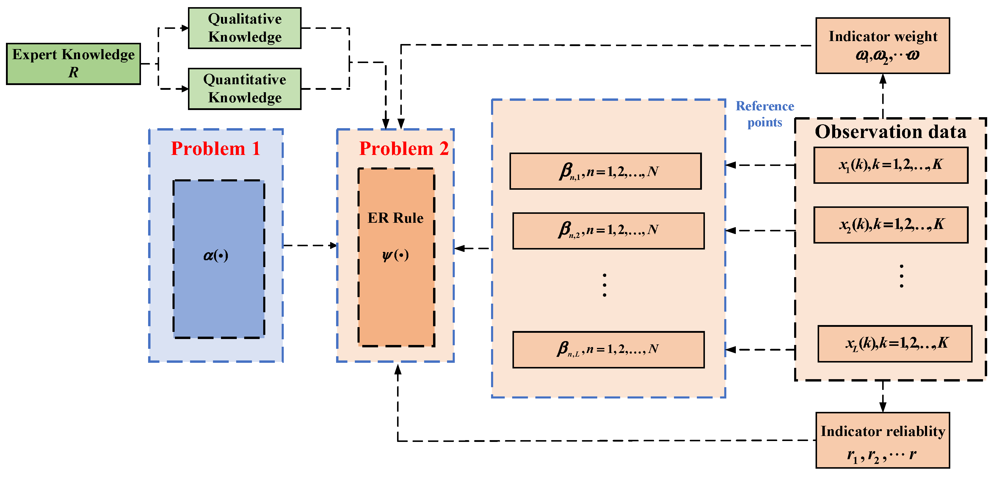
2.2. Evidence-Related ER Rules Problem Description
The problem description of the ER rule where evidence is not independent is as follows.
Problem 1: (Correlation Heterogeneity): Evidence diversity in complex systems introduces computational interference in correlation coefficient determination when inter-evidence correlations exist, resulting in biased diagnosis. This necessitates advanced correlation modeling capable of simultaneous linear/nonlinear relationship characterization.
Problem 2: (Uncertainty Propagation): Multi-source fusion processes are inherently affected by hybrid uncertainties in system test data. Uncertain data analysis becomes a critical research priority for probabilistic reasoning systems. While the ER framework has been widely adopted for uncertainty management, its inherent independence assumption remains problematic in practical engineering contexts. System complexity and functional interdependencies frequently violate the evidence independence requirement mandated by conventional ER implementations. Consequently, evidence correlations are systematically unaddressed in traditional ER frameworks, and the reliability of the fault diagnosis results is compromised. This work therefore focuses on reasoning process enhancement under correlated evidence conditions.
The evidence-related ER rule is structured as follows (
Figure 1).
The modeling of expert knowledge R includes the following. (1) For quantitative information , denotes the reference value of , and , where denotes the amount of quantitative information and denotes the number of reference values. The expert establishes a mapping relationship between the numerical quantities and the reference values , i.e., . Let and be the largest and the smallest reference values, respectively, then can be converted to the following belief distribution: , where . Assuming that the reference value is equivalent to the evaluation level of the belief distribution, the quantitative information can be uniformly expressed as , where denotes the belief degree that the quantitative information is evaluated as the level . (2) For qualitative information, there is subjective judgment by experts in combination with domain knowledge to give a belief degree relative to the reference values.
2.3. Evidence-Related ER Framework
2.3.1. Correlation Coefficient Calculation
Due to the variety of data types in actual engineering, including linear data and nonlinear data, there are a lot of irrelevant or redundant data in these data, and irrelevant or redundant data often affect the evaluation results. Therefore, it is important to choose an appropriate correlation coefficient calculation method, which must be able to handle both linear and nonlinear data. The correlation coefficient calculation process is as follows:
where
and
are input,
represents the correlation coefficients, and
is the correlation coefficient calculation function.
2.3.2. Establishment of Evidence-Related ER Rule Framework
After the appropriate correlation coefficient calculation method is selected, the improved ER rule using the correlation coefficient is
where
is the new ER rule inference,
is the output,
is
evidence, and
is the set of parameters required by the model.
where
denotes the optimization function;
is the optimization parameter set.
To summarize, to construct an evidence-related evidential inference rule framework, it is necessary to solve new ER rules and optimize functions, weight, reliability, and parameter sets.
3. ER Rule with Maximum Information Coefficient
In this section, the ER rule is modeled and inferred by the maximum information coefficient. In
Section 3.1, the greatest mutual information coefficient is used to compute the evidence correlation coefficient. The modeling of the maximum information coefficient ER rule (MICER Rule) and the optimization process are carried out in
Section 3.2.
3.1. Correlation Analysis
Mutual information (MI) is the foundation upon which the maximum information coefficient is constructed. It is capable of mining non-functional dependencies between variables in great detail in addition to measuring both linear and nonlinear relationships between variables in vast amounts of data. Due to the diversity of data variables (including linear and nonlinear, etc.) in health status evaluation in actual engineering, the characteristics of the evidence obtained from the data are consistent with it. Therefore, this paper chooses MIC to measure the degree of association between evidence. The larger the MIC value between two variables, the stronger the correlation; otherwise, the weaker the correlation.
The maximum information coefficient is mainly calculated by mutual information and grid division methods. Mutual information can be regarded as the uncertainty reduced by one random variable because another random variable is known, and it is mainly used to measure the degree of association between linear or nonlinear variables. Let
and
be random variables, where
is the number of samples, then the mutual information is defined as
where
and
are the marginal density functions;
is the joint probability density function;
is the mutual information of variables
and
. The correlation between two variables is stronger the more mutual information there is between them.
Assuming that
is a finite set of ordered pairs, the definition partition
divides the value range of the variable
into
segments and divides the value range of
into
segments, and
is the grid of
. Mutual information
is calculated internally in grid division. There are many grid division methods with the same
, and they take the maximum value of
in different divisions as the value of mutual information of the division
. The formula for the maximum mutual information of
under the division
is defined as
where
means that the data
is divided using
.
denotes the maximum mutual information value of data
under
delimitation.
denotes the mutual information value of data
under
delimitation.
Even though the maximum information coefficient uses mutual information to represent the grid’s quality, it is not simply to estimate the mutual information. The maximum normalized
values obtained under different divisions form a feature matrix, and the feature matrix is defined as
, and the calculation formula is
Then, the maximum information coefficient is defined as
where
is the upper limit value of grid division
. Generally, it is believed that the effect is best when
, so this value is also used in the experiment.
In summary, the MIC calculation is divided into three steps:
Step 1: Given and , the maximum mutual information value is computed by gridding the scatter diagram made up of with columns and j rows;
Step 2: The greatest mutual information value is normalized;
Step 3: The MIC value is determined by taking the highest value of mutual information at various scales.
Remark 1. Equations (13) and (16)–(19) are computed by default in this paper for ordered discrete variables.
3.2. MICER Rule
The ER rule characterizes evidence through a reliable weighted belief distribution (WBDR) to supplement the belief distribution (BD) introduced in the D-S evidence theory and is established by performing orthogonal sum operations on the weighted belief distribution (WBD) and WBDR. It is a generalized Bayesian inference process or a general joint probabilistic inference method. Simultaneously, it offers a straightforward and reliable reasoning process that can handle a range of uncertainties.
Suppose the FoD is defined as
, where
is the
system state,
. The power set of
consists of
subsets, described by
Suppose there are
pieces of evidence
; the
piece of evidence can be modeled as a basic probability distribution as follows:
where
is a subset of
.
is the belief assigned to state
by evidence
.
Assume that
represents the weight of
and that the following is the basic probability mass of
supports
:
where
is the
piece of evidence.
Therefore, the underlying probability mass distribution of
can be denoted as
where
is expressed as the remaining support determined by the weight of evidence, which means
.
denotes the power set of
. There is
because the equality constraint
always holds. Therefore, (23) is a generalized probability distribution form.
We first provide the basic ER rule lemma, which follows the work of Yang and Xu [
7].
Lemma 1 (basic form of ER rule). For two correlated pieces of evidence and , assuming their reliability is given by and , respectively, their basic probability mass distribution is shown in (23). Then, the probability that and jointly support can be calculated as follows:
In (24), is the joint probability that and jointly support . denotes the unnormalized total probability mass of from and . The symbol is as a subset of . In (25), and denote the reliabilities of and . The first term is called the bounded sum of the individual supports of by and , respectively. The basic probability mass that and support is indicated by and , respectively. denotes the interdependence of and . In addition, is called the orthogonal sum of the common support of and , measuring the degree of all intersected supports on proposition . Symbols and are also arbitrary subsets of .
We provide the following lemma for the recursive ER rule to generalize:
Lemma 2 (recursive form of the ER rule). For pieces of relevant evidence , assuming their reliability is given by , their basic probability mass distribution is represented like in (23). Then, by iteratively using the following equation, the likelihood that independent pieces of evidence support overall can be produced:
where represents the joint probability that the first pieces of evidence supports , . is the joint probability mass assignment of the first pieces of evidence to . and represent the unnormalized combined probability mass of and in the previous pieces of evidence. There are and , respectively. , , and are also subsets of . The aforementioned analysis indicates that new synthetic evidence
can be produced by combining the
pieces of evidence. Its probability distribution looks like this:where
is the joint probability that
pieces of evidence support
. The expected utility of
is computed as follows, assuming that the utility of state
is
: Remark 2. Parameter definitions and methodological considerations.
The parameters addressed in this subsection are weight and reliability of evidence and reference level. The parameters of evidence weight and reliability serve distinct roles: weights represent the subjective importance of evidence (e.g., decision-maker preferences for specific indicators), while reliability quantifies its objective credibility (e.g., sensor measurement precision or expert judgment consistency). There are many methods in setting the weight of evidence, including the subjective assignment method (e.g., expert experience method, preference rule mapping), the objective calculation method (e.g., information entropy method, data-driven method), the combination weighting method (subjective-objective combination of weights), and the dynamic adjustment mechanism (e.g., conflict feedback adjustment, utility-sensitive weights). Methods of setting reliability are based on information consistency calculations (e.g., fluctuation analysis, perturbation factor method models), modeling of statistical properties (e.g., probability density function method, interval reliability), and expert calibration methods (e.g., reliability scoring, cross-validation methods). Different weights and reliability setting methods apply to different scenarios, so it is necessary to choose suitable setting methods according to specific application scenarios when setting weights and reliability. In this paper, reference levels are set by experts in conjunction with domain knowledge.
Remark 3. Algorithmic robustness and parameterization strategy.
The orthogonal sum operator in evidential reasoning (ER) inherently embeds a residual belief assignment mechanism that redistributes residual uncertainty to the identification framework, providing strong resistance to interference perturbations. This intrinsic robustness, empirically validated in prior studies [
33,
34], buffers against weight variations—experiments demonstrate ≤ 5% confidence deviation under ±20% weight perturbations. Consequently, the current methodology intentionally excludes weight optimization. Similarly, reliability calibration (reflecting objective evidence credibility) falls beyond conventional ER optimization scopes. Reference grades, derived from domain expert knowledge in this study, are retained without optimization to preserve interpretability and operational transparency. These deliberate design choices align with industrial diagnostic requirements where explainability and stability outweigh marginal accuracy gains from parametric tuning.
5. Conclusions
This study proposes the MICER framework to address two critical limitations of conventional evidential reasoning (ER) in fault diagnosis: the independent assumption of evidence and the inability to quantify nonlinear evidence correlations. The key methodological contributions are systematically summarized as follows.
1. Unified Correlation Analysis for Heterogeneous Evidence
The framework introduces a novel approach to simultaneously process linear and nonlinear interdependencies among multi-source sensor data. By integrating maximum mutual information coefficient (MIC) theory, it overcomes the constraints of currently available ER methods that consider correlation, effectively capturing complex interaction patterns (e.g., inverse temperature–humidity relationships in fault diagnosis where environmental effects need to be taken into account) that traditional linear metrics fail to detect.
2. Joint Probability Modeling with MIC Quantification
A nonparametric joint probability modeling mechanism is established through MIC’s adaptive grid partitioning, enabling correlation quantification without prior assumptions on evidence distributions. This allows robust fusion of heterogeneous sensor data (vibration, thermal, chemical) under uncertainty, as validated in flywheel system diagnostics.
3. Generalized ER Rule Reformulation
The conventional Dempster combination rule is extended through recursive computation architectures that embed MIC-derived correlation weights. This reformulation resolves conflicts arising from unmodeled evidence dependencies while maintaining compatibility with existing ER implementations. The recursive form specifically addresses multi-stage fusion scenarios in static systems, avoiding combinatorial complexity growth.
Two critical research frontiers emerge from this work: first, the development of causal correlation discrimination frameworks to address spurious sensor data associations, particularly crucial for systems with time-varying operating conditions; second, the integration of online learning mechanisms to enable MICER’s autonomous adaptation to emerging fault patterns in evolving industrial systems. Future investigations should prioritize establishing standardized protocols for correlation hierarchy analysis and validation benchmarks for next-generation evidence fusion systems.


