


Advancing Rice Disease Detection in Farmland with an Enhanced YOLOv11 Algorithm

Abstract
1. Introduction
- We introduced an enhanced attention module, SPPFLKC (an advanced version of the SPPF module with added Large-Separable-Kernel Attention and Convolution capabilities). When integrated with the backbone and neck, it significantly improves multi-scale feature extraction capabilities.
- We added the C3k2-CFCGLU block (modified C3k2 block with CAFormer and CGLU), which consists of CAFormer (an efficient vision model combining convolution and self-attention) and the CGLU (an improved channel mixer), reducing computational complexity and channel redundancy while increasing the model’s proficiency in capturing fine-grained local features.
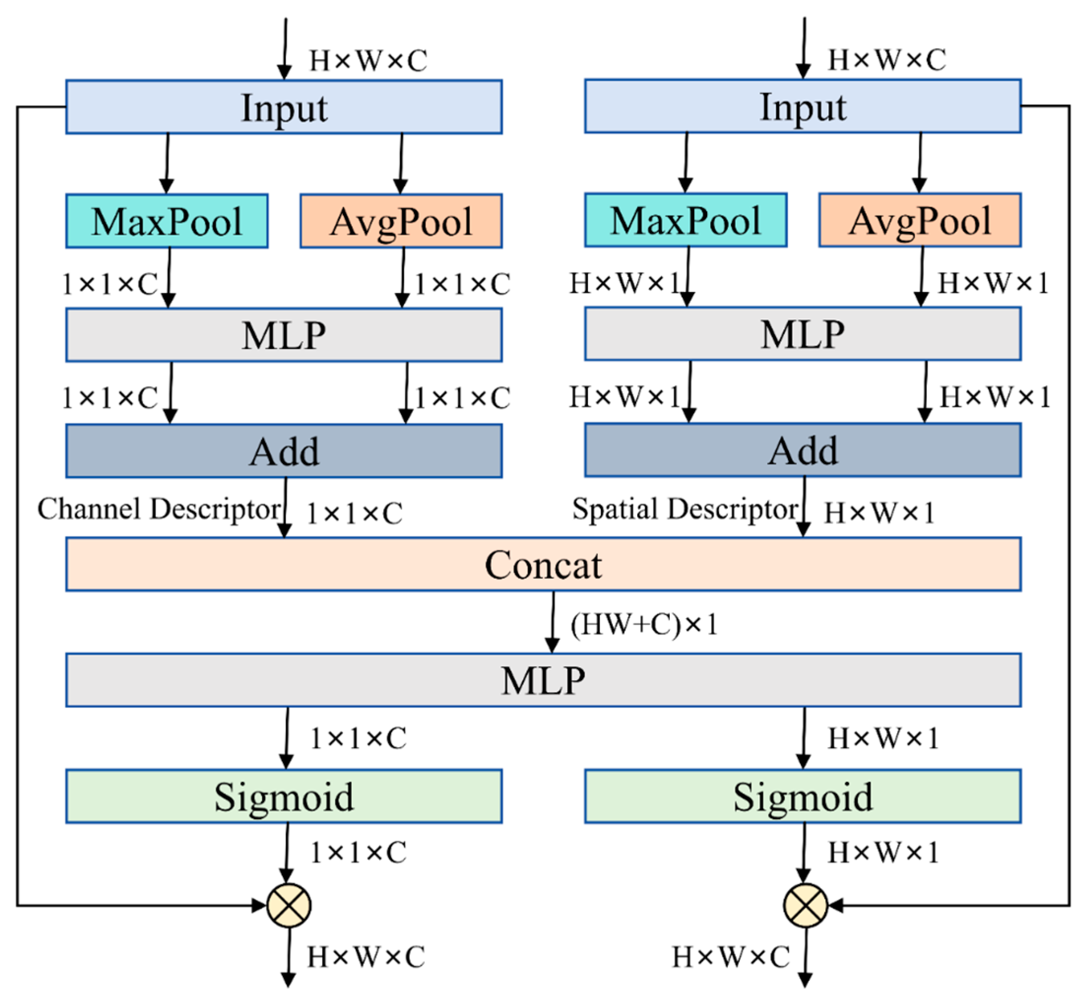
- We designed the C3k2-CSCBAM (modified C3k2 block with CSCBAM) block based on the CSCBAM (Channel–Spatial Combined Attention Module), which reduces the training overhead and improves the network’s capability to learn target features in complex farmland environments.
- We added the 320 × 320 scale LSDECD detection head, improved with detail-enhanced convolution, to enhance small-object detection capabilities while meeting lightweight requirements.
2. Model Architecture and Improvements
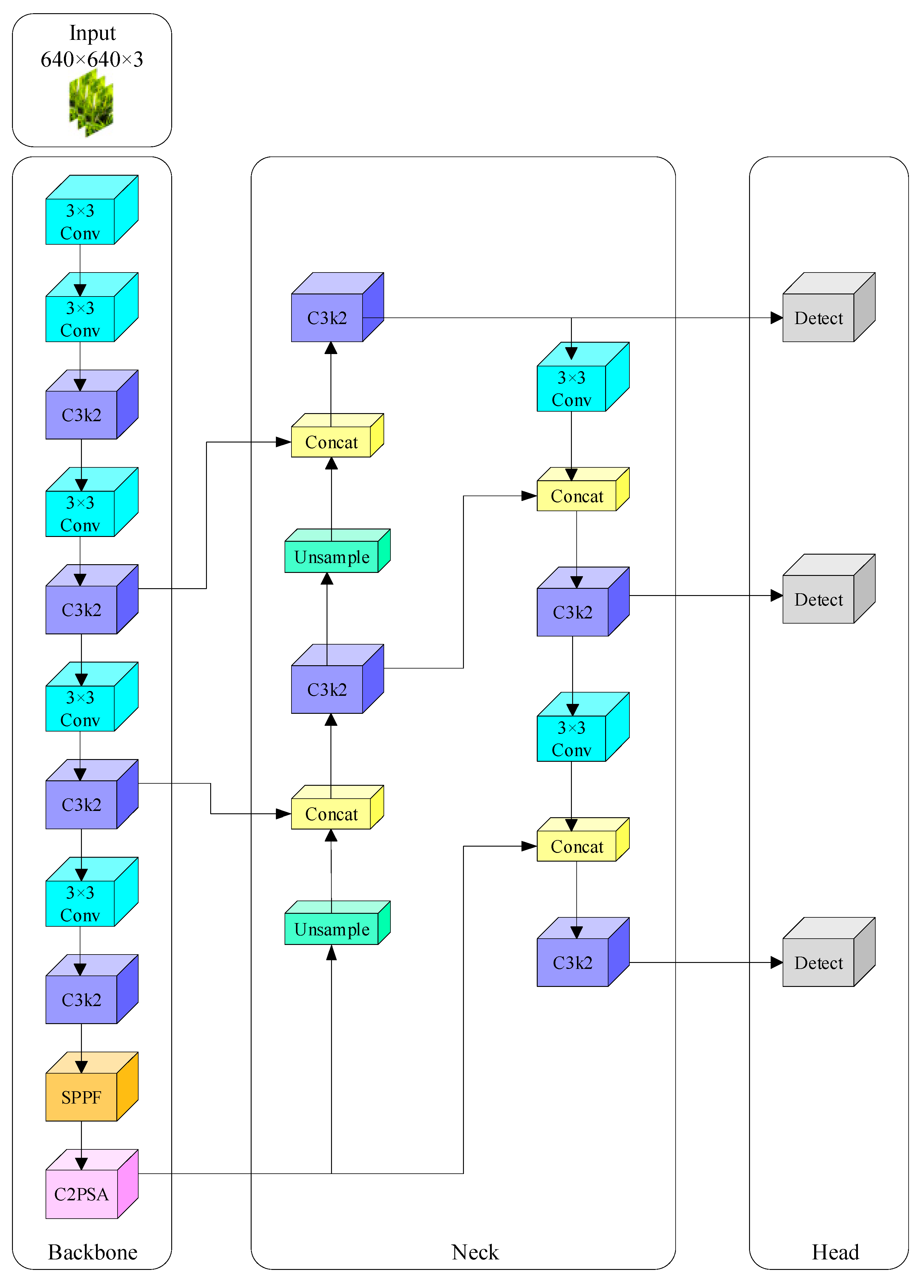
2.1. YOLOv11 Architecture
2.2. YOLOv11-RD Architecture
2.3. SPPFLKC Attention Mechanism
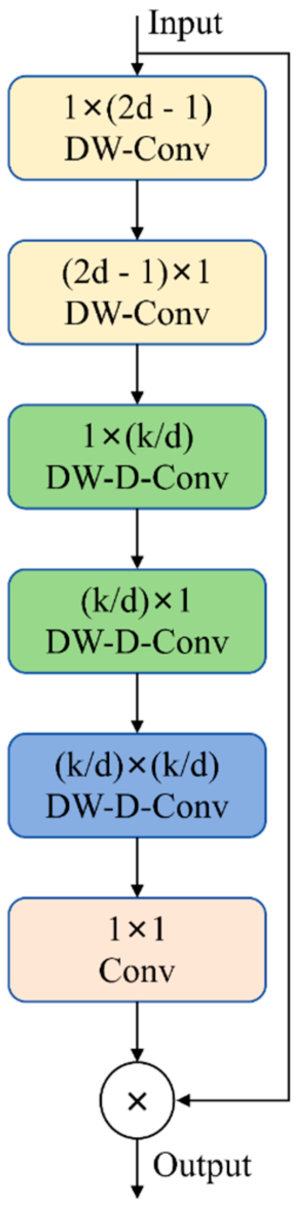
2.3.1. LSKAC
2.3.2. SPPFLKC
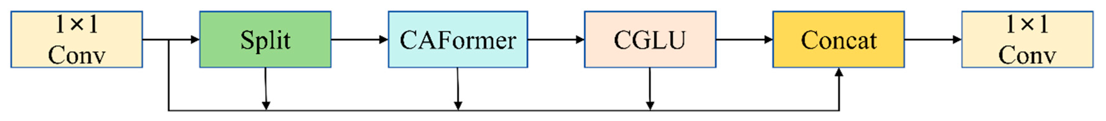
2.4. C3k2-CFCGLU
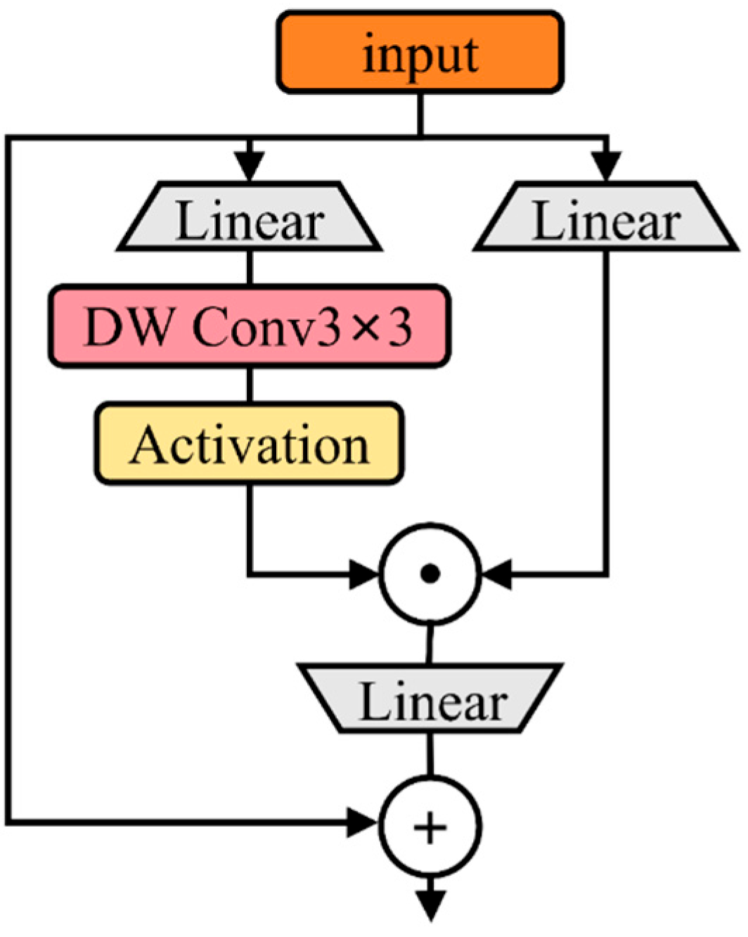
2.4.1. CAFormer
2.4.2. CGLU
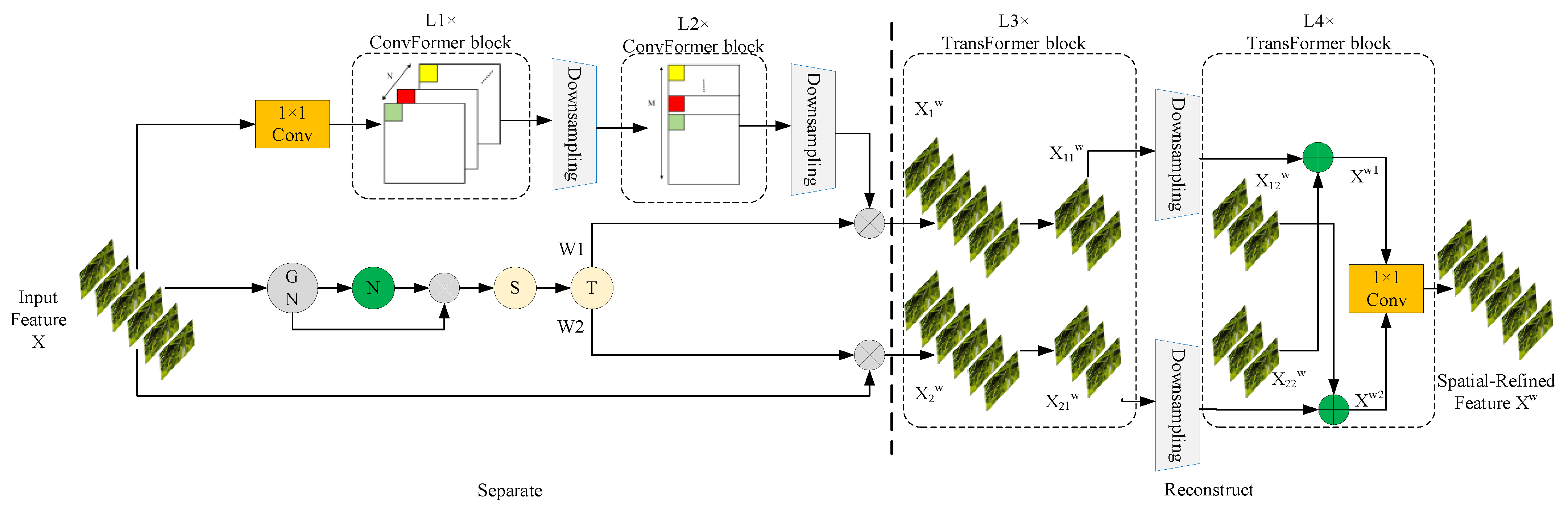
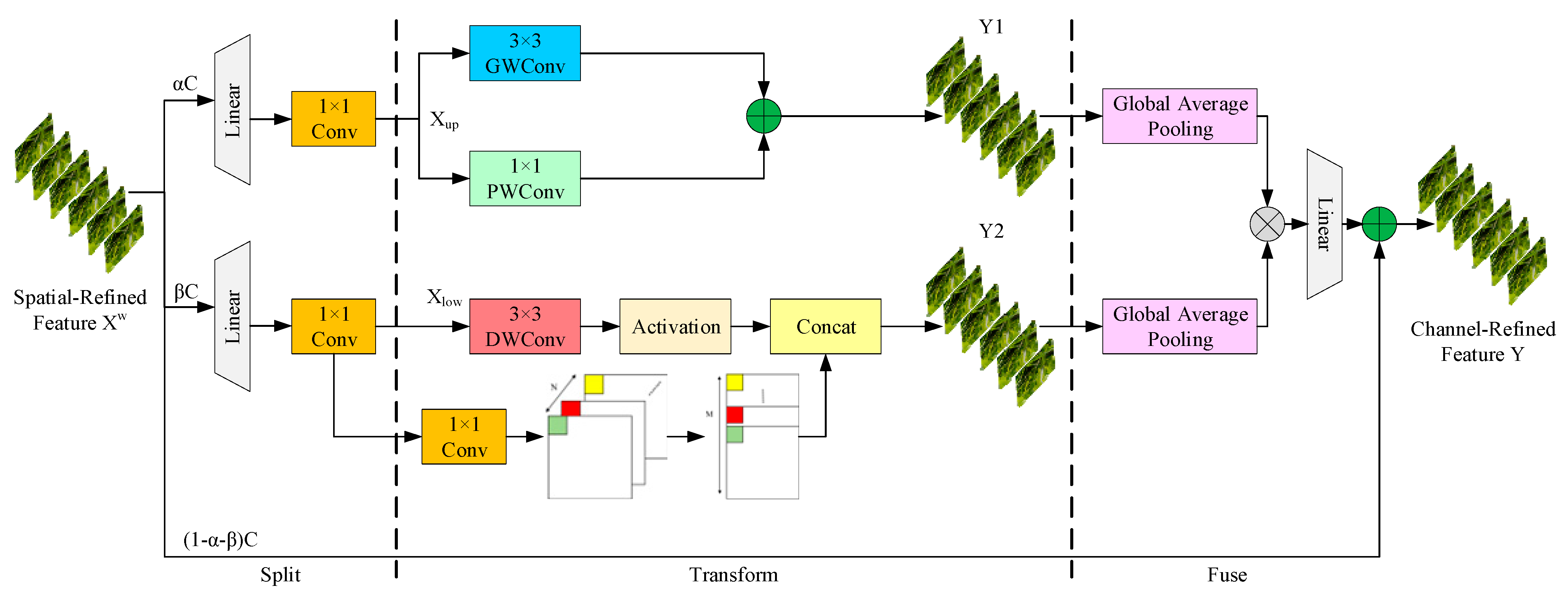
2.5. C3k2-CSCBAM
2.6. Small Detection Layer
3. Results and Discussion
3.1. Dataset Preparation
3.2. Experimental Environment and Parameter Setup
3.3. Evaluation Metrics
3.4. Evaluation Results
3.4.1. SPPFLKC Validity Analysis
3.4.2. Model Comparison Experiment
3.4.3. Ablation Experiment
3.4.4. Cross-Validation Experiment
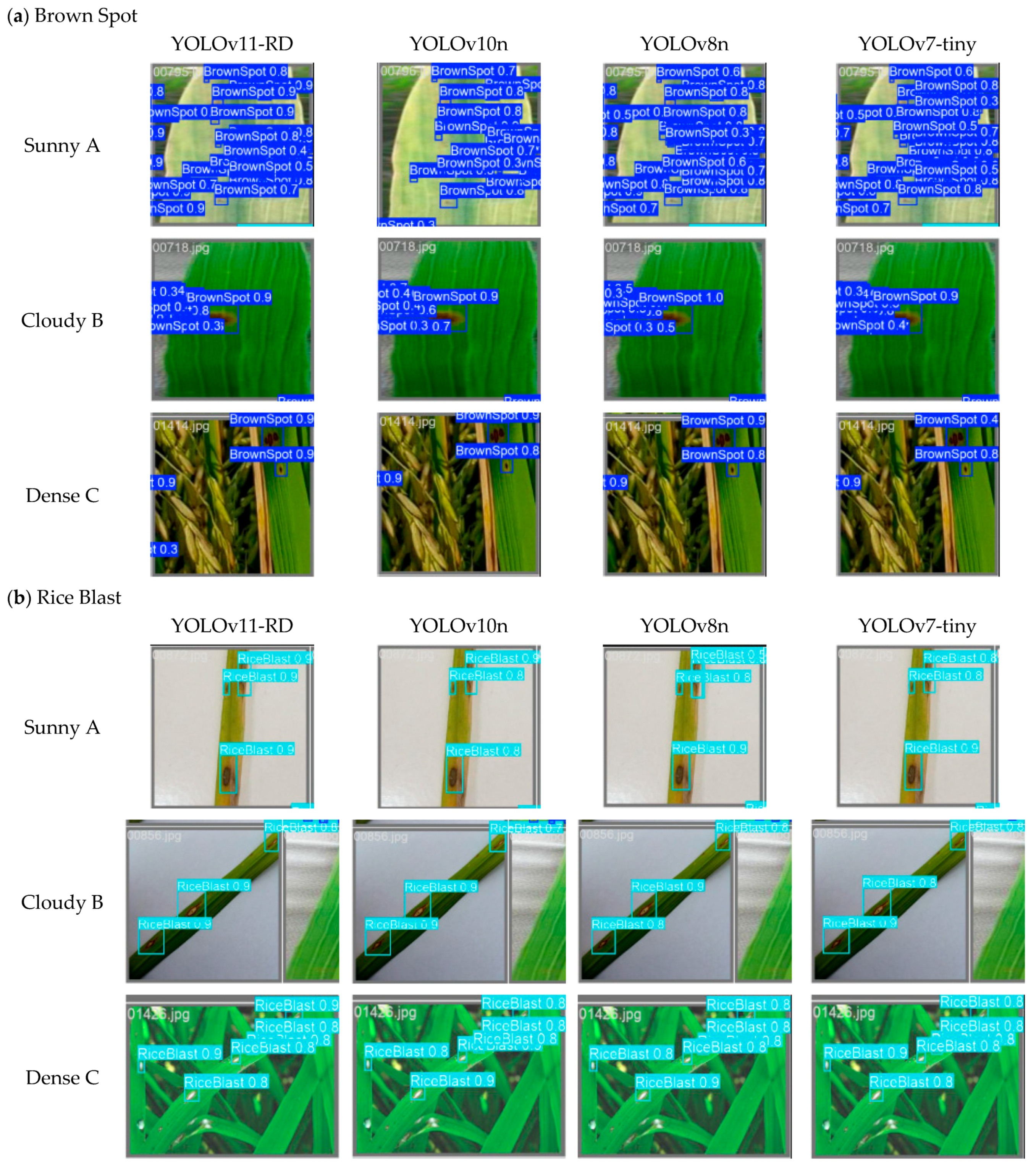
3.5. Algorithm Effect Verification
3.6. Data Analysis
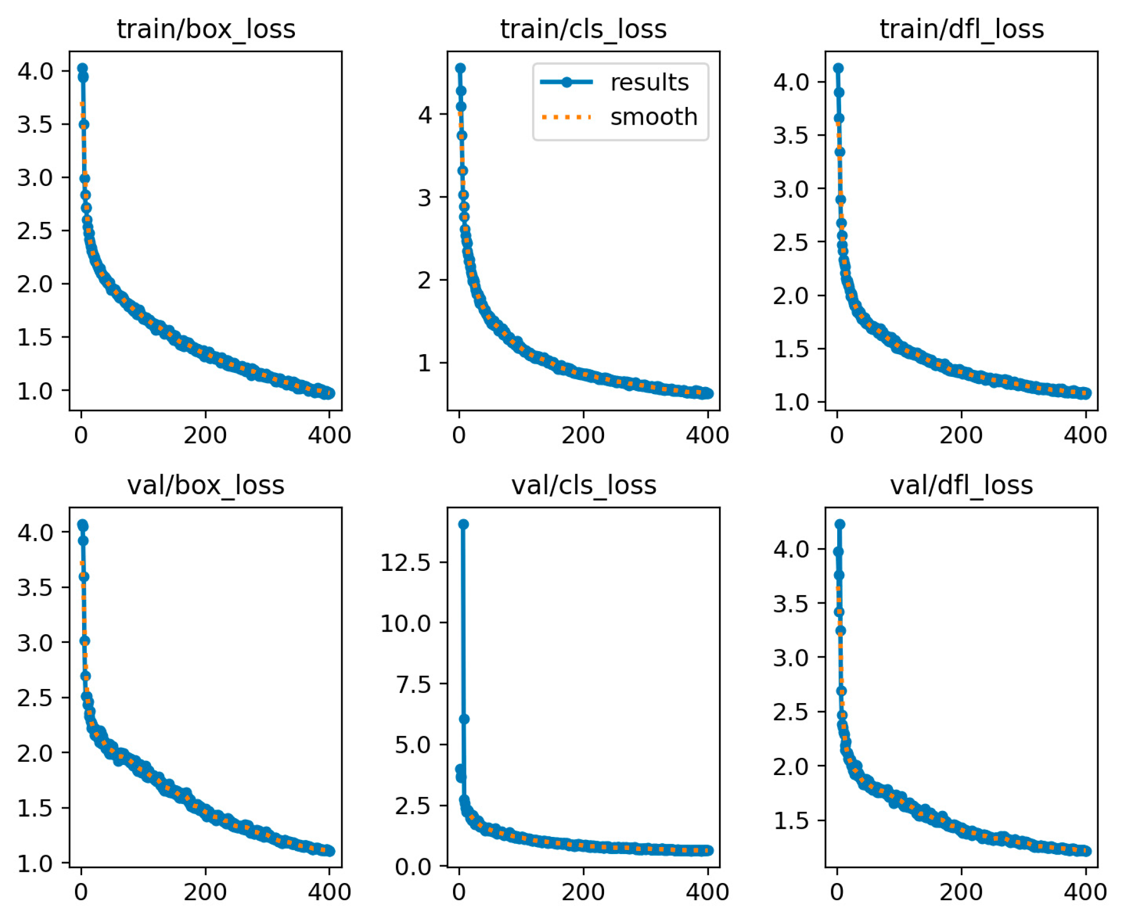
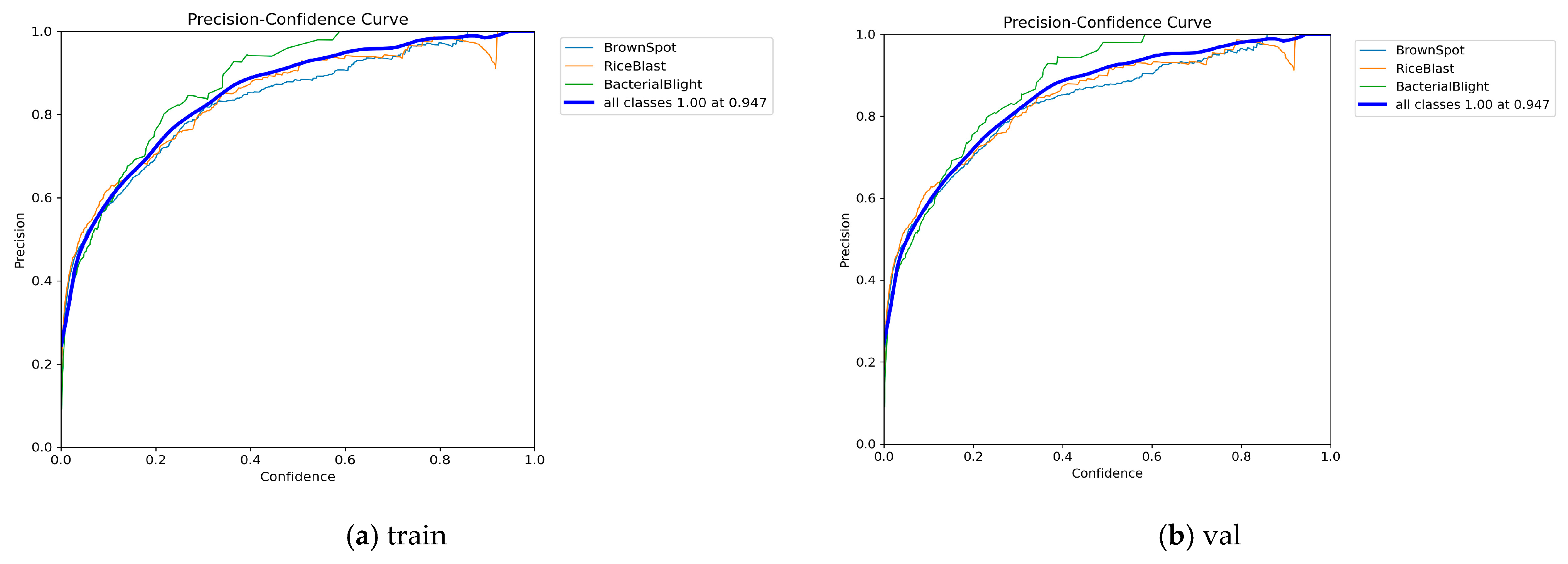
3.7. Performance Assessment of Training, Validation, and Test Sets
3.8. Practical Deployment Validation
4. Conclusions
Author Contributions
Funding
Institutional Review Board Statement
Informed Consent Statement
Data Availability Statement
Conflicts of Interest
Abbreviations
| RD | Rice disease |
| YOLOv11 | You Only Look Once version 11 |
| SPPFLKC | Modified SPPF module with Large-Separable-Kernel Attention with Convolution |
| C3k2-CFCGLU | Modified C3k2 block with CAFormer and CGLU |
| CAFormer | Convolutional Attention Former |
| CGLU | Convolutional Gated Linear Unit |
| C3k2-CSCBAM | Modified C3k2 block with CSCBAM |
| CSCBAM | Channel–Spatial Combined Attention Module |
| C3k2 | Cross Stage Partial Bottleneck with 3 Conv layers and Key-point Detection |
| LZKAC | Large-Kernel Attention with Convolution |
| SPPF | Spatial Pyramid Pooling Fast |
| LKA | Large-Kernel Attention |
| LSKA | Large-Separable-Kernel Attention |
| MaxPool2d | Max pooling 2D |
| AvgPool2d | Average pooling 2D |
| SCConv | Split Convolution |
| GN | Group Normalization |
| DW | Deep Width |
| GWConv | Group Convolution |
| PWConv | Point-by-point Convolution |
| MLP | Multi-layer perceptron |
| BN | Batch Normalization |
| ReLU | Rectified Linear Unit |
| mAP | Mean average precision |
References
- Erenstein, O.; Jaleta, M.; Mottaleb, K.A.; Sonder, K.; Donovan, J.; Braun, H.-J. Global trends in wheat production, consumption and trade. In Wheat Improvement: Food Security in a Changing Climate; Springer International Publishing Cham: Berlin/Heidelberg, Germany, 2022; pp. 47–66. [Google Scholar] [CrossRef]
- Wei, T.; Xu, L.J.S.D. China food security comprehensive assessment dataset 2012–2022. Sci. Data 2025, 12, 621. [Google Scholar] [CrossRef] [PubMed]
- Rudiyanto; Minasny, B.; Shah, R.M.; Che Soh, N.; Arif, C.; Indra Setiawan, B. Automated near-real-time mapping and monitoring of rice extent, cropping patterns, and growth stages in Southeast Asia using Sentinel-1 time series on a Google Earth Engine platform. Remote Sens. 2019, 11, 1666. [Google Scholar] [CrossRef]
- Xu, S.; Zhu, X.; Chen, J.; Zhu, X.; Duan, M.; Qiu, B.; Wan, L.; Tan, X.; Xu, Y.N.; Cao, R. A robust index to extract paddy fields in cloudy regions from SAR time series. Remote Sens. Environ. 2023, 285, 113374. [Google Scholar] [CrossRef]
- Fahad, S.; Adnan, M.; Noor, M.; Arif, M.; Alam, M.; Khan, I.A.; Ullah, H.; Wahid, F.; Mian, I.A.; Jamal, Y. Advances in rice research for abiotic stress tolerance. In Major Constraints for Global Rice Production; Elsevier: Amsterdam, The Netherlands, 2019; pp. 1–22. [Google Scholar] [CrossRef]
- Qi, G.; Zhang, Y.; Wang, K.; Mazur, N.; Liu, Y.; Malaviya, D. Small object detection method based on adaptive spatial parallel convolution and fast multi-scale fusion. Remote Sens. 2022, 14, 420. [Google Scholar] [CrossRef]
- Bansal, M.; Kumar, M.; Kumar, M.; Kumar, K. An efficient technique for object recognition using Shi-Tomasi corner detection algorithm. Soft Comput. 2021, 25, 4423–4432. [Google Scholar] [CrossRef]
- Wang, G.; Zhuang, Y.; Chen, H.; Liu, X.; Zhang, T.; Li, L.; Dong, S.; Sang, Q. FSoD-Net: Full-scale object detection from optical remote sensing imagery. IEEE Trans. Geosci. Remote Sens. 2021, 60, 1–18. [Google Scholar] [CrossRef]
- Vijayakumar, A.; Vairavasundaram, S. Yolo-based object detection models: A review and its applications. Multimed. Tools Appl. 2024, 83, 83535–83574. [Google Scholar] [CrossRef]
- Diwan, T.; Anirudh, G.; Tembhurne, J.V. Object detection using YOLO: Challenges, architectural successors, datasets and applications. Multimed. Tools Appl. 2023, 82, 9243–9275. [Google Scholar] [CrossRef]
- Wang, C.-Y.; Bochkovskiy, A.; Liao, H.-Y.M. YOLOv7: Trainable bag-of-freebies sets new state-of-the-art for real-time object detectors. In Proceedings of the IEEE/CVF Conference on Computer Vision and Pattern Recognition, Vancouver, BC, Canada, 17–24 June 2023; pp. 7464–7475. [Google Scholar]
- Liu, W.; Anguelov, D.; Erhan, D.; Szegedy, C.; Reed, S.; Fu, C.-Y.; Berg, A.C. Ssd: Single shot multibox detector. In Proceedings of the Computer Vision–ECCV 2016: 14th European Conference, Amsterdam, The Netherlands, 11–14 October 2016; pp. 21–37. [Google Scholar]
- Girshick, R. Fast r-cnn. In Proceedings of the IEEE International Conference on Computer Vision, Santiago, Chile, 7–13 December 2015; pp. 1440–1448. [Google Scholar]
- Ren, S.; He, K.; Girshick, R.; Sun, J. Faster R-CNN: Towards real-time object detection with region proposal networks. IEEE Trans. Pattern Anal. Mach. Intell. 2016, 39, 1137–1149. [Google Scholar] [CrossRef]
- Cai, Z.; Vasconcelos, N. Cascade r-cnn: Delving into high quality object detection. In Proceedings of the IEEE Conference on Computer Vision and Pattern Recognition, Salt Lake City, UT, USA, 18–23 June 2018; pp. 6154–6162. [Google Scholar]
- Xue, Z.; Xu, R.; Bai, D.; Lin, H. YOLO-tea: A tea disease detection model improved by YOLOv5. Forests 2023, 14, 415. [Google Scholar] [CrossRef]
- Jia, L.; Wang, T.; Chen, Y.; Zang, Y.; Li, X.; Shi, H.; Gao, L. MobileNet-CA-YOLO: An improved YOLOv7 based on the MobileNetV3 and attention mechanism for Rice pests and diseases detection. Agriculture 2023, 13, 1285. [Google Scholar] [CrossRef]
- Sangaiah, A.K.; Yu, F.-N.; Lin, Y.-B.; Shen, W.-C.; Sharma, A. UAV T-YOLO-rice: An enhanced tiny YOLO networks for rice leaves diseases detection in paddy agronomy. IEEE Trans. Netw. Sci. Eng. 2024, 11, 5201–5216. [Google Scholar] [CrossRef]
- Li, H.; Wu, A.; Jiang, Z.; Liu, F.; Luo, M. Improving object detection in YOLOv8n with the C2f-f module and multi-scale fusion reconstruction. In Proceedings of the 2024 IEEE 6th Advanced Information Management, Communicates, Electronic and Automation Control Conference (IMCEC), Chongqing, China, 24–26 May 2024; pp. 374–379. [Google Scholar] [CrossRef]
- Lau, K.W.; Po, L.-M.; Rehman, Y.A.U. Large separable kernel attention: Rethinking the large kernel attention design in cnn. Expert Syst. Appl. 2024, 236, 121352. [Google Scholar] [CrossRef]
- Guo, M.H.; Lu, C.Z.; Liu, Z.N.; Cheng, M.M.; Hu, S.M. Visual attention network. Comput. Vis. Media 2023, 9, 733–752. [Google Scholar] [CrossRef]
- Li, J.; Wen, Y.; He, L. Scconv: Spatial and channel reconstruction convolution for feature redundancy. In Proceedings of the IEEE/CVF Conference on Computer Vision and Pattern Recognition, Vancouver, BC, Canada, 17–24 June 2023; pp. 6153–6162. [Google Scholar]
- Dai, Y.; Li, C.; Su, X.; Liu, H.; Li, J. Multi-scale depthwise separable convolution for semantic segmentation in street–road scenes. Remote Sens. 2023, 15, 2649. [Google Scholar] [CrossRef]
- Zhang, A.; Jia, L.; Wang, J.; Wang, C. Sar image classification using gated channel attention based convolutional neural network. Remote Sens. 2023, 15, 362. [Google Scholar] [CrossRef]
- Dong, J.; Zhuang, D.; Huang, Y.; Fu, J. Advances in multi-sensor data fusion: Algorithms and applications. Sensors 2009, 9, 7771–7784. [Google Scholar] [CrossRef]
- Lv, H.; Chen, J.; Pan, T.; Zhang, T.; Feng, Y.; Liu, S. Attention mechanism in intelligent fault diagnosis of machinery: A review of technique and application. Measurement 2022, 199, 111594. [Google Scholar] [CrossRef]
- Ma, R.; Chen, J.; Feng, Y.; Zhou, Z.; Xie, J. ELA-YOLO: An efficient method with linear attention for steel surface defect detection during manufacturing. Adv. Eng. Inform. 2025, 65, 103377. [Google Scholar] [CrossRef]
- Ni, H.; Shi, Z.; Karungaru, S.; Lv, S.; Li, X.; Wang, X.; Zhang, J. Classification of typical pests and diseases of Rice based on the ECA attention mechanism. Agriculture 2023, 13, 1066. [Google Scholar] [CrossRef]
- Hao, W.; Ren, C.; Han, M.; Zhang, L.; Li, F.; Liu, Z. Cattle body detection based on YOLOv5-EMA for precision livestock farming. Animals 2023, 13, 3535. [Google Scholar] [CrossRef] [PubMed]
- Wang, C.; Wang, Y. Sensors. SLGA-YOLO: A Lightweight Castings Surface Defect Detection Method Based on Fusion-Enhanced Attention Mechanism and Self-Architecture. Sensors 2024, 24, 4088. [Google Scholar] [CrossRef]
- Mahaadevan, V.; Narayanamoorthi, R.; Gono, R.; Moldrik, P. Automatic identifier of socket for electrical vehicles using SWIN-transformer and SimAM attention mechanism-based EVS YOLO. IEEE Access 2023, 11, 111238–111254. [Google Scholar] [CrossRef]
- Zhai, S.; Shang, D.; Wang, S.; Dong, S. DF-SSD: An improved SSD object detection algorithm based on DenseNet and feature fusion. IEEE Access 2020, 8, 24344–24357. [Google Scholar] [CrossRef]
- Wang, S.; Jiang, H.; Li, Z.; Yang, J.; Ma, X.; Chen, J.; Tang, X. Phsi-rtdetr: A lightweight infrared small target detection algorithm based on UAV aerial photography. Drones 2024, 8, 240. [Google Scholar] [CrossRef]
- Qi, K.; Yang, Z.; Fan, Y.; Song, H.; Liang, Z.; Wang, S.; Wang, F. Detection and classification of Shiitake mushroom fruiting bodies based on Mamba YOLO. Sci. Rep. 2025, 15, 15214. [Google Scholar] [CrossRef]
- Huang, Y.; Liu, Z.; Zhao, H.; Tang, C.; Liu, B.; Li, Z.; Wan, F.; Qian, W.; Qiao, X. YOLO-YSTs: An Improved YOLOv10n-Based Method for Real-Time Field Pest Detection. Agronomy 2025, 15, 575. [Google Scholar] [CrossRef]
- Li, P.; Zhou, J.; Sun, H.; Zeng, J. RDRM-YOLO: A High-Accuracy and Lightweight Rice Disease Detection Model for Complex Field Environments Based on Improved YOLOv5. Agriculture 2025, 15, 479. [Google Scholar] [CrossRef]


| Category | Number |
|---|---|
| Rice Blast | 2353 |
| Brown Spot | 1215 |
| Bacterial Blight | 1432 |
| Category | Number |
|---|---|
| Brown Spot | 1600 |
| Rice Blast | 1200 |
| Bacterial Blight | 1200 |
| Parameters | Settings | Parameters | Settings |
|---|---|---|---|
| Optimizer | SGD | lrf | 0.01 |
| Epochs | 300 | weight_decay | 0.005 |
| Batchsize | 32 | momentum | 0.937 |
| Workers | 4 | warmup_epochs | 3 |
| Imgsz | 640 | warmup_momentum | 0.8 |
| lr0 | 0.01 | close_mosaic | 0 |
| Model | Precision (%) | Recall (%) | map50 (%) | mAP 50-95 (%) | GFLOPs | Params /M |
|---|---|---|---|---|---|---|
| SE | 94.1 | 91.2 | 94.8 | 73.3 | 8.7 | 12.13 |
| ELA | 93.7 | 90.3 | 93.4 | 72.9 | 8.5 | 10.28 |
| ECA | 93.6 | 90.1 | 92.9 | 73.4 | 8.4 | 10.02 |
| EMA | 93.4 | 89.9 | 92.5 | 72.8 | 8.5 | 10.45 |
| LSKA | 93.8 | 90.5 | 93.7 | 72.5 | 8.8 | 13.06 |
| SimAM | 93.9 | 90.8 | 94.3 | 73.6 | 8.7 | 12.25 |
| SPPFLKC | 94.4 | 91.6 | 95.1 | 74.8 | 8.6 | 11.05 |
| Model | Precision (%) | Recall (%) | mAP50 (%) | mAP50-95 (%) | GFLOPs | Params /M |
|---|---|---|---|---|---|---|
| SSD | 79.2 | 26.3 | 45.9 | 57.1 | 36.8 | 47.2 |
| Faster R-CNN | 83.7 | 72.4 | 75.8 | 63.6 | 205.2 | 105 |
| RT-DETR | 91.5 | 91.3 | 92.1 | 72.4 | 9.6 | 11.8 |
| Mamba-YOLO | 91.9 | 90.7 | 91.3 | 71.5 | 10.5 | 12.4 |
| YOLOv5s | 80.3 | 76.2 | 79.6 | 58.2 | 17.4 | 28.1 |
| YOLOv7-tiny | 81.6 | 78.3 | 82.3 | 64.3 | 6.6 | 6.8 |
| YOLOv8n | 90.8 | 88.6 | 90.8 | 70.8 | 9.3 | 15.8 |
| YOLOv10n | 91.3 | 90.5 | 92.5 | 72.6 | 9.2 | 12.3 |
| YOLOv11n | 92.4 | 88.5 | 93.3 | 68.4 | 8.9 | 11.5 |
| YOLO-YSTs | 83.2 | 83.2 | 86.8 | 41.3 | 8.8 | 3.02 |
| RDRM-YOLO | 94.3 | 89.6 | 93.5 | 70.5 | 10.2 | 7.9 |
| YOLOv11-RD | 94.6 | 93.1 | 95.8 | 76.3 | 7.8 | 6.92 |
| SDL | SPPFLKC | C3k2-CFCGLU | C3k2-CSCBAM | Precision (%) | Recall (%) | mAP50 (%) | mAP 50-95 (%) | GFLOPs | Params /M |
|---|---|---|---|---|---|---|---|---|---|
| × | × | × | × | 92.4 | 88.5 | 93.3 | 68.4 | 8.9 | 11.5 |
| √ | × | × | × | 93.7 | 90.5 | 94.6 | 70.3 | 9.1 | 12.14 |
| × | √ | × | × | 94.1 | 91.8 | 94.9 | 71.3 | 9.1 | 12.05 |
| × | × | √ | × | 93.7 | 91.2 | 94.6 | 73.9 | 8.3 | 7.73 |
| × | × | × | √ | 93.6 | 90.4 | 94.5 | 74.7 | 8.2 | 7.61 |
| √ | √ | × | × | 94.2 | 90.8 | 94.9 | 74.8 | 9.4 | 13.39 |
| √ | × | √ | × | 93.4 | 91.3 | 95.1 | 73.3 | 8.4 | 8.73 |
| √ | × | × | √ | 94.3 | 91.5 | 95.2 | 73.2 | 8.3 | 8.48 |
| × | √ | √ | × | 94.2 | 90.8 | 94.6 | 74.1 | 8.3 | 8.53 |
| × | √ | × | √ | 94.1 | 91.5 | 95.4 | 74.4 | 8.4 | 8.61 |
| × | × | √ | √ | 93.9 | 91.4 | 94.7 | 75.9 | 7.3 | 5.18 |
| √ | √ | √ | × | 93.8 | 91.8 | 95.2 | 75.3 | 8.7 | 9.39 |
| √ | √ | × | √ | 93.8 | 92.3 | 95.3 | 75.2 | 8.6 | 9.12 |
| √ | × | √ | √ | 94.3 | 92.5 | 95.3 | 76.1 | 7.6 | 5.56 |
| × | √ | √ | √ | 94.5 | 92.9 | 95.5 | 75.5 | 7.7 | 5.72 |
| √ | √ | √ | √ | 94.6 | 93.1 | 95.8 | 76.3 | 7.8 | 6.92 |
| Folds | Precision (%) | Recall (%) | mAP50 (%) | mAP50-95 (%) |
|---|---|---|---|---|
| 1 | 94.5 | 93.1 | 95.7 | 76.1 |
| 2 | 94.6 | 93.0 | 95.9 | 76.3 |
| 3 | 94.8 | 93.2 | 95.5 | 76.2 |
| 4 | 94.7 | 93.3 | 95.6 | 76.5 |
| 5 | 94.4 | 92.9 | 95.8 | 76.4 |
| Average | 94.6 | 93.1 | 95.7 | 76.3 |
| Group | Model | Precision (%) | Recall (%) | mAP50-95 (%) |
|---|---|---|---|---|
| A (sunny) | YOLOv11-RD | 96.2 | 94.8 | 78.5 |
| YOLOv10n | 92.7 | 89.3 | 71.2 | |
| YOLOv8n | 90.5 | 87.6 | 69.8 | |
| YOLOv7-tiny | 85.4 | 82.1 | 63.4 | |
| B (cloudy) | YOLOv11-RD | 95.8 | 93.5 | 77.9 |
| YOLOv10n | 91.4 | 88.7 | 70.5 | |
| YOLOv8n | 89.2 | 85.9 | 68.1 | |
| YOLOv7-tiny | 83.6 | 80.3 | 61.2 | |
| C (dense) | YOLOv11-RD | 94.3 | 92.1 | 76.1 |
| YOLOv10n | 89.8 | 86.4 | 67.8 | |
| YOLOv8n | 87.5 | 84.2 | 65.3 | |
| YOLOv7-tiny | 81.9 | 78.0 | 59.7 |
| Set | Precision (%) | Recall (%) | mAP50 (%) | mAP50-95 (%) |
|---|---|---|---|---|
| Train | 95.2 | 92.8 | 95.7 | 75.8 |
| Val | 95.1 | 93.1 | 95.8 | 76.3 |
| Test | 95.1 | 93.3 | 95.8 | 75.9 |
Disclaimer/Publisher’s Note: The statements, opinions and data contained in all publications are solely those of the individual author(s) and contributor(s) and not of MDPI and/or the editor(s). MDPI and/or the editor(s) disclaim responsibility for any injury to people or property resulting from any ideas, methods, instructions or products referred to in the content. |
© 2025 by the authors. Licensee MDPI, Basel, Switzerland. This article is an open access article distributed under the terms and conditions of the Creative Commons Attribution (CC BY) license (https://creativecommons.org/licenses/by/4.0/).
Share and Cite
Teng, H.; Wang, Y.; Li, W.; Chen, T.; Liu, Q. Advancing Rice Disease Detection in Farmland with an Enhanced YOLOv11 Algorithm. Sensors 2025, 25, 3056. https://doi.org/10.3390/s25103056
Teng H, Wang Y, Li W, Chen T, Liu Q. Advancing Rice Disease Detection in Farmland with an Enhanced YOLOv11 Algorithm. Sensors. 2025; 25(10):3056. https://doi.org/10.3390/s25103056
Chicago/Turabian StyleTeng, Hongxin, Yudi Wang, Wentao Li, Tao Chen, and Qinghua Liu. 2025. "Advancing Rice Disease Detection in Farmland with an Enhanced YOLOv11 Algorithm" Sensors 25, no. 10: 3056. https://doi.org/10.3390/s25103056
APA StyleTeng, H., Wang, Y., Li, W., Chen, T., & Liu, Q. (2025). Advancing Rice Disease Detection in Farmland with an Enhanced YOLOv11 Algorithm. Sensors, 25(10), 3056. https://doi.org/10.3390/s25103056