
Parameter Self-Adjusting Single-Mode Fiber Nutation Coupling Algorithm Based on Fuzzy Control

 ,
,
Abstract
1. Introduction
2. Working Principle and Simulation Analysis
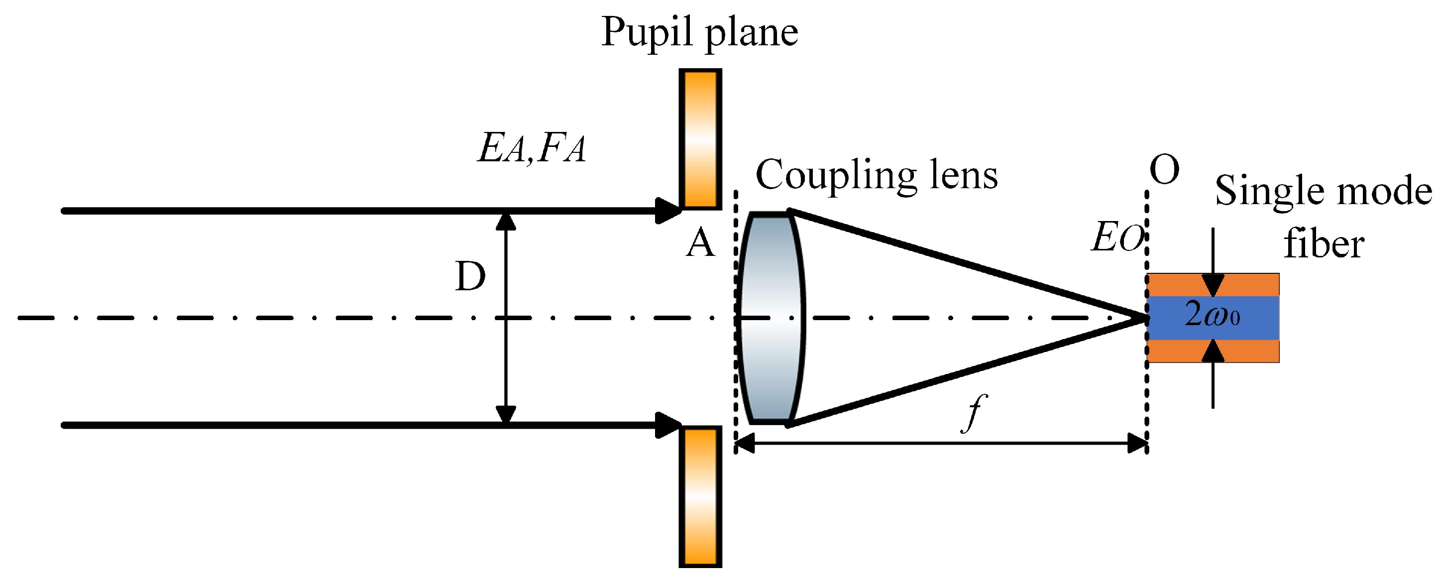
2.1. SMF Coupling Principle
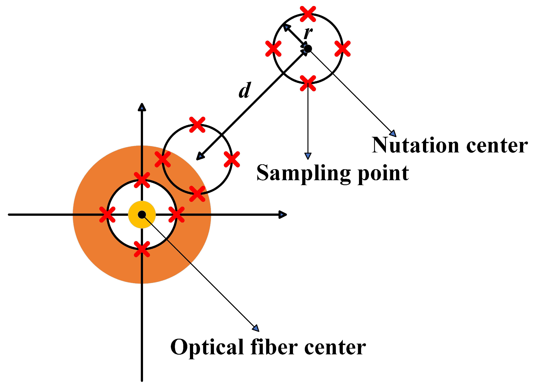
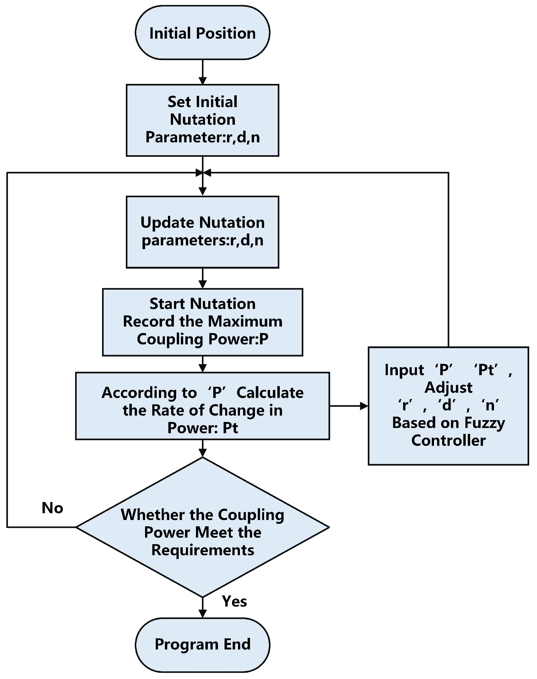
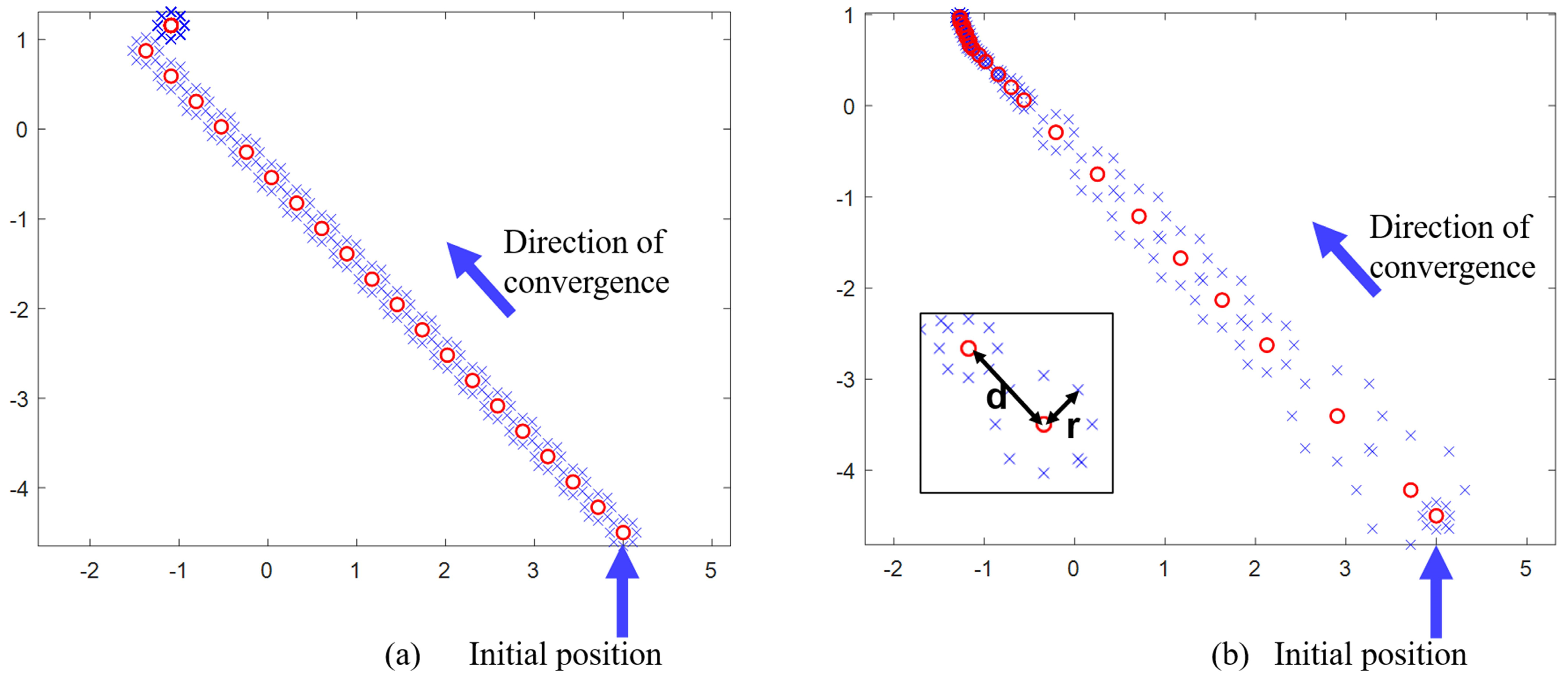
2.2. Fiber Nutation Algorithm
- (1)
- The algorithm initializes parameter setting, and sets the scanning center , the nutation radius , nutation step length , and the number of sampling points per revolution.
- (2)
- Output the control quantity: calculate the control quantity , where:
- (3)
- Move the scanning center: move the scanning center in the direction of the maximum coupling efficiency according to the set nutation step length , that is,
- (4)
- Repeat steps (2) to (3). The above process can be represented by Figure 2.
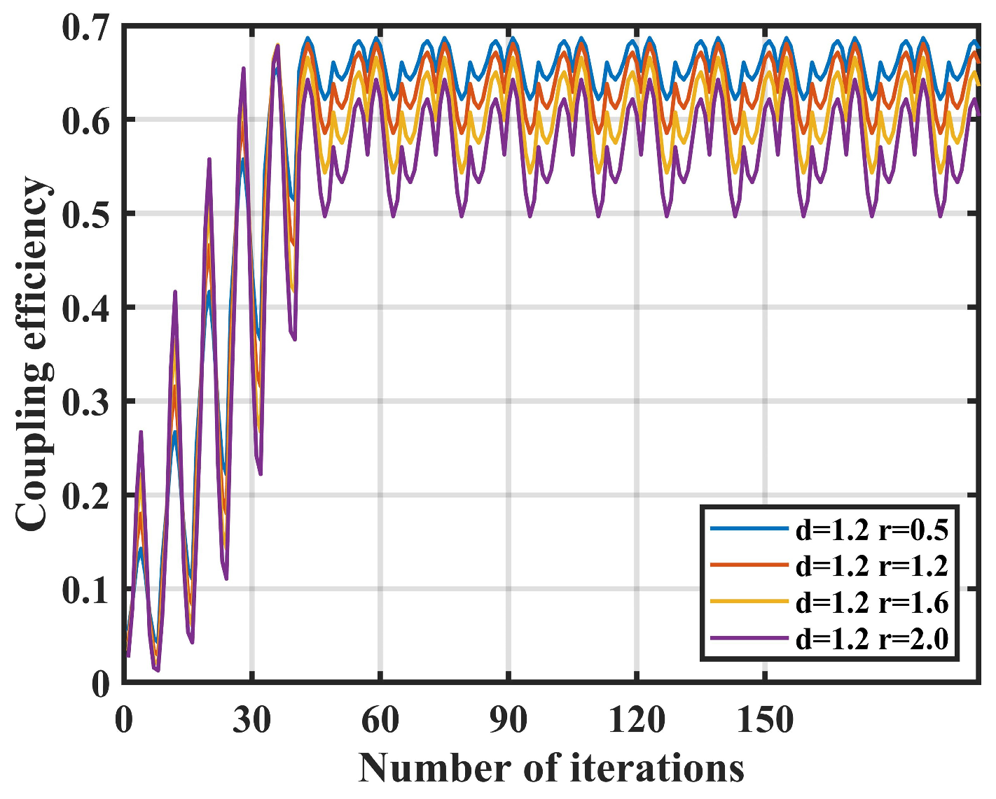
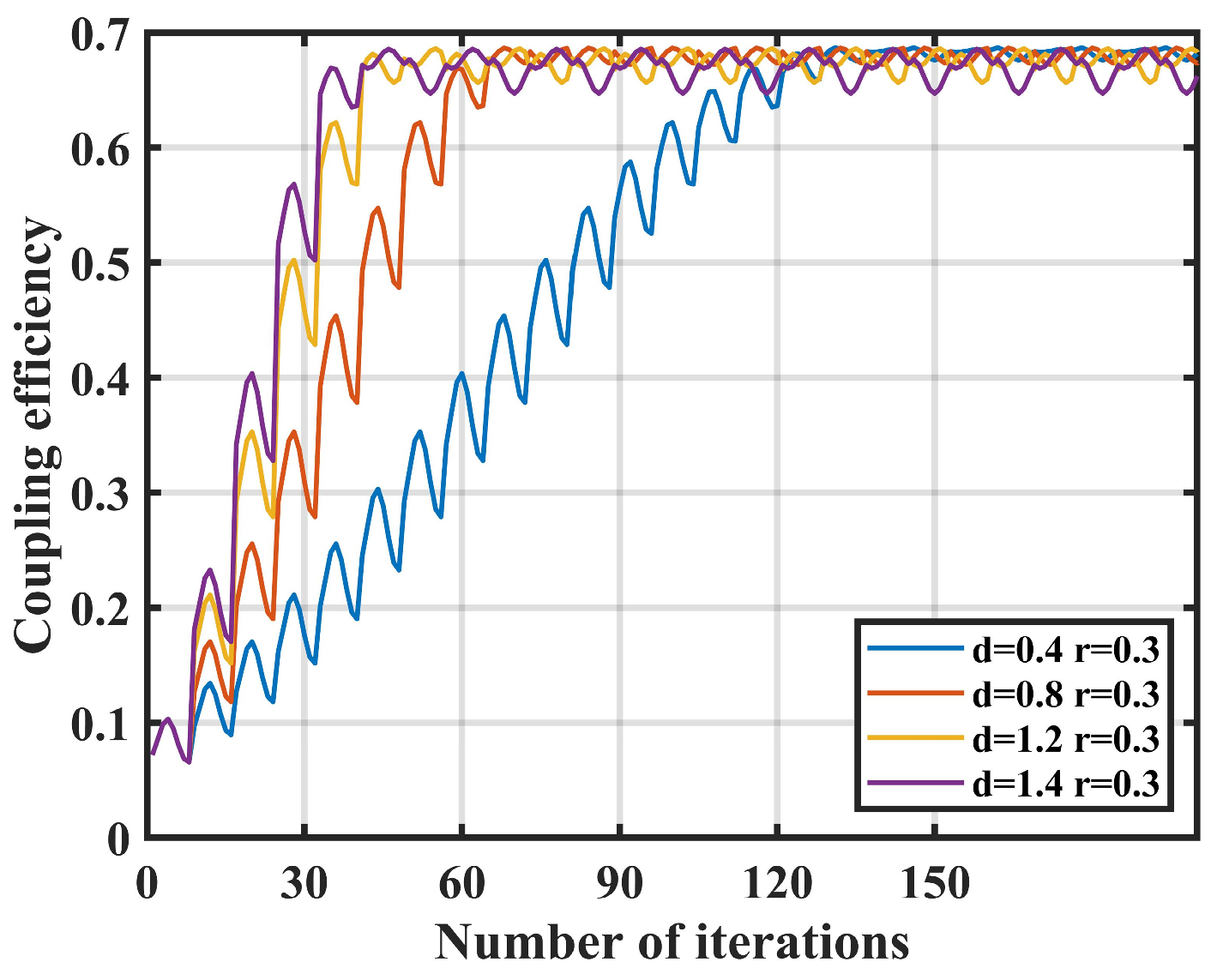
2.3. Analysis of the Influence of Nutation Parameters on Coupling Performance
- (1)
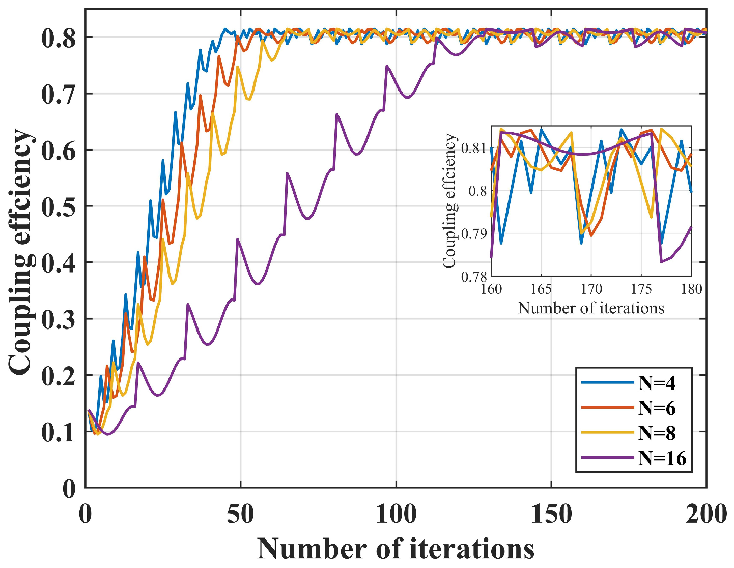
- Coupling speed: the time required for the SMF coupling power to reach its maximum value from the initial value after the algorithm is activated.
- (2)
- Coupling stability: the fluctuation of coupling power after steady-state coupling is achieved, described by the steady-state standard deviation, denoted as .
- (3)
- Coupling efficiency: the steady-state coupling power divided by the input power, with the input power set to 1 in the simulation.
2.4. Fuzzy Control Algorithm
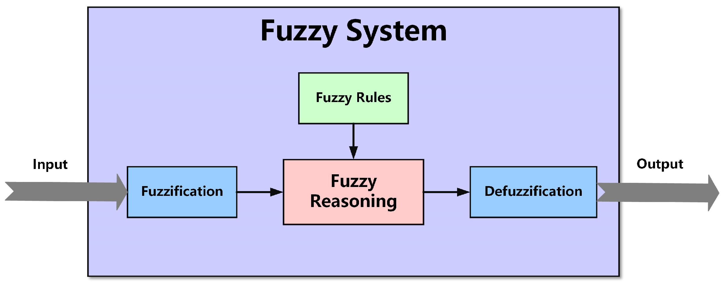
- (1)
- Fuzzification: the primary objective of this step is to convert system input values into fuzzy set values. These fuzzy sets are usually represented by linguistic variables (such as low, medium, and high), which describe the different degrees or ranges of the input variable.
- (2)
- Fuzzy reasoning: after fuzzification, the system applies a set of fuzzy rules to make decisions. These rules define the relationship between inputs and outputs. The fuzzy control algorithm utilizes these rules to determine the corresponding output actions based on specific input combinations. Calculate the membership of a rule premise.
- (3)
- Defuzzification: this step converts the outputs from the fuzzy inference stage into precise control action values. The defuzzification process generates the final non-fuzzy output value, which serves as the actual control input for the fiber nutation algorithm by considering all possible output fuzzy sets and their respective membership degrees. The formula is:
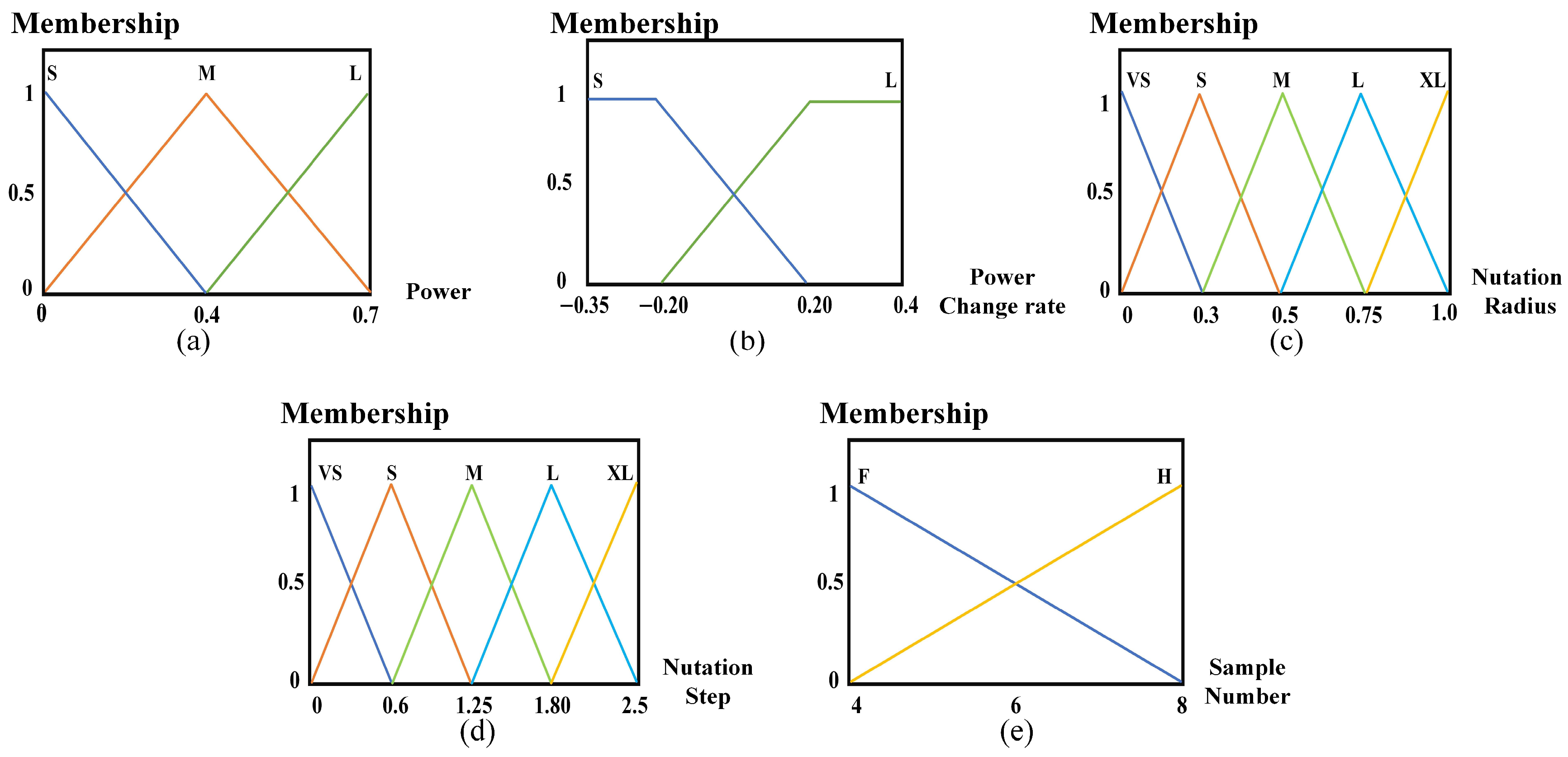
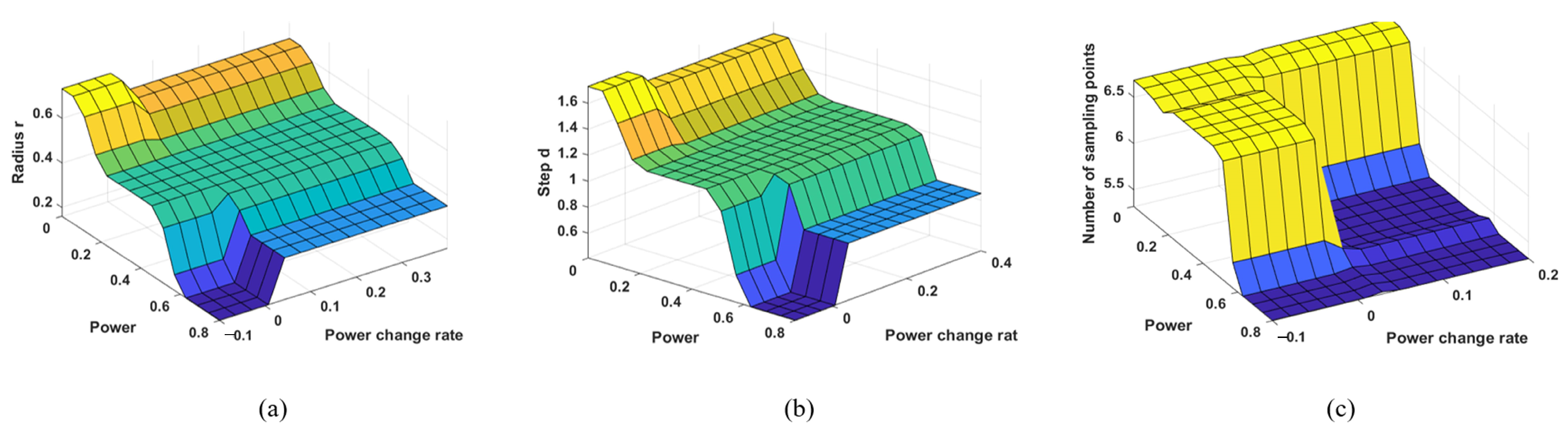
2.5. Fuzzy Controller Design
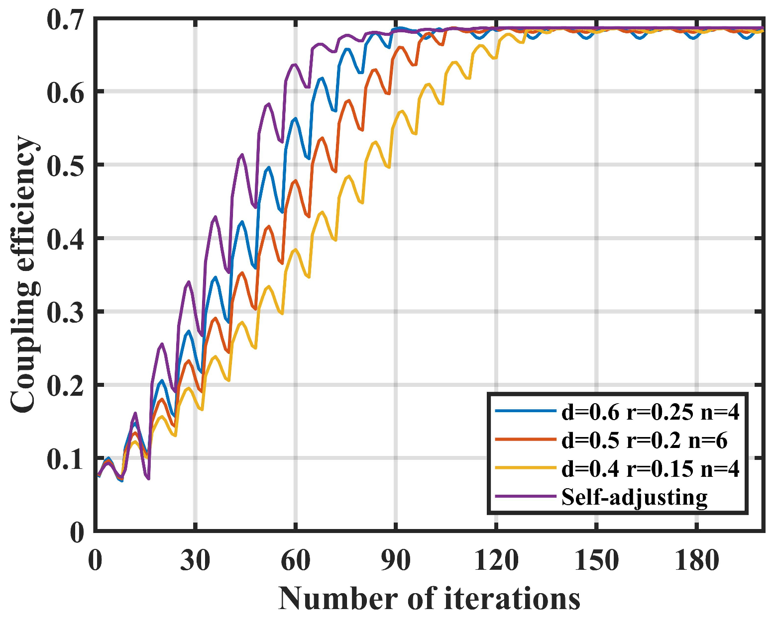
2.6. Simulation and Analysis of Nutation Coupling Algorithm for SMF with Parameter Self-Adjusting Based on Fuzzy Control
2.7. Summary
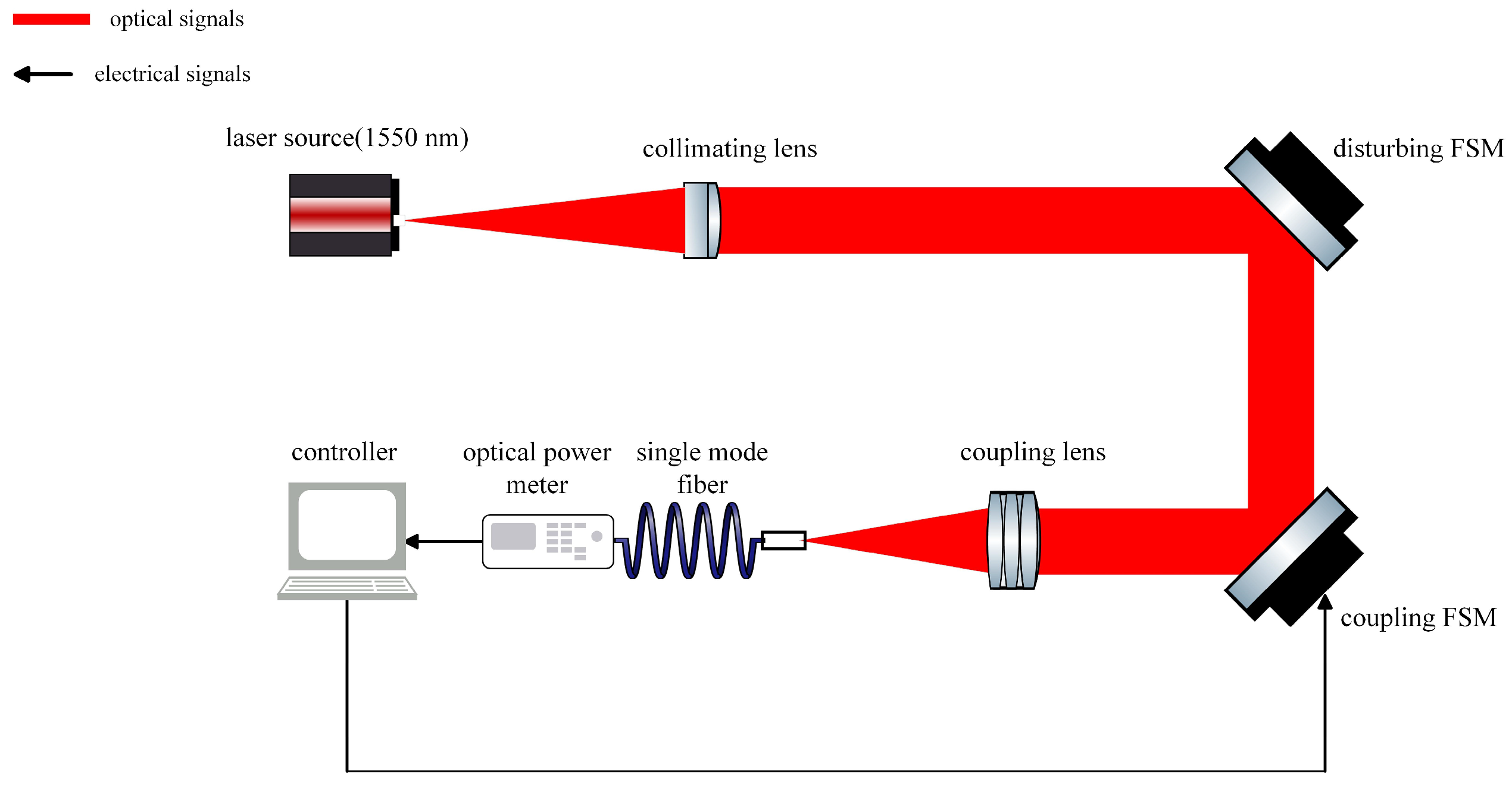
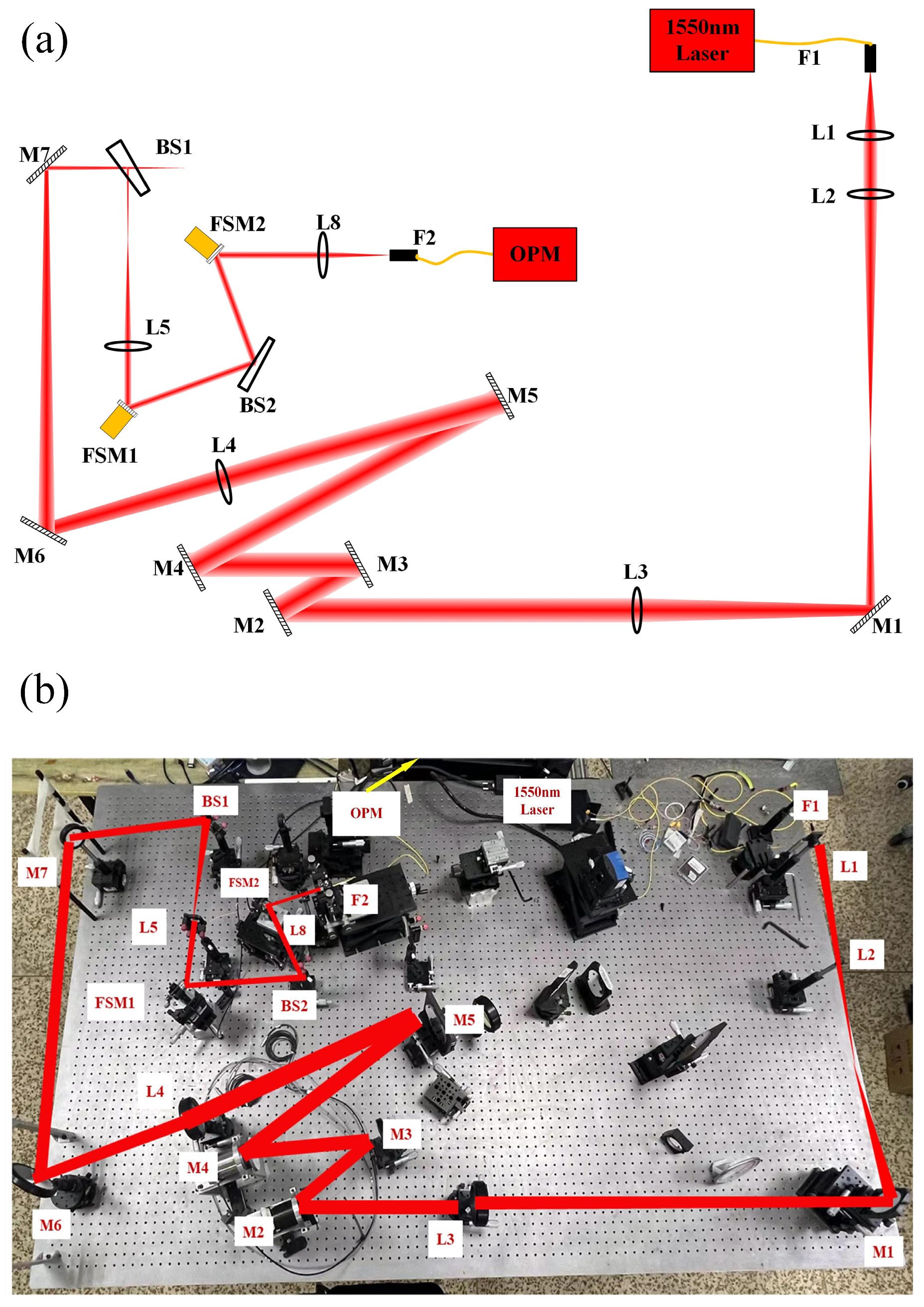
3. Experiment
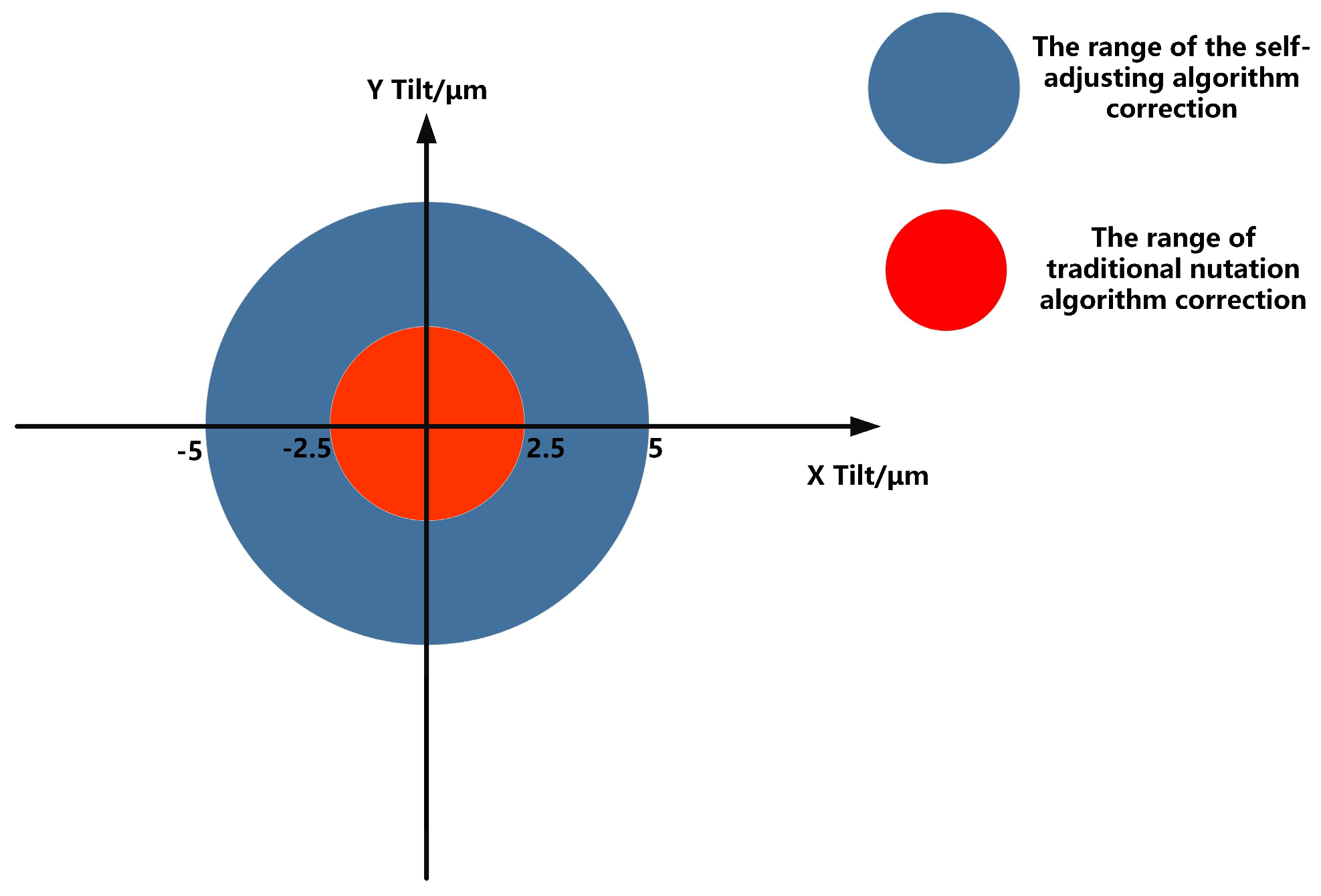
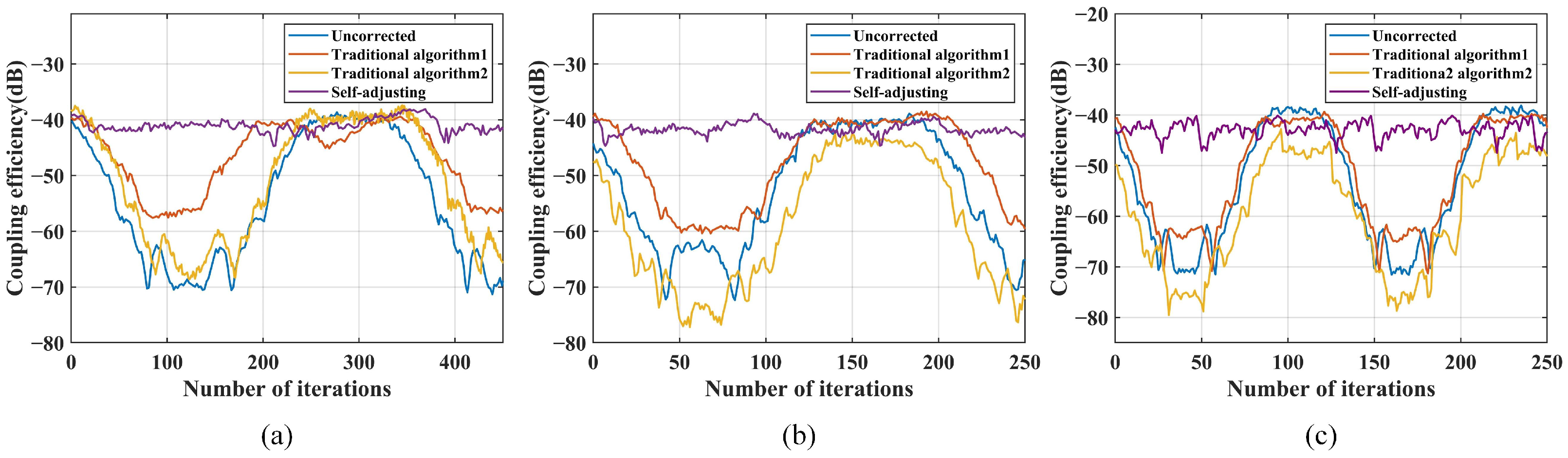
3.1. Static Coupling Experiment of Parameter Self-Adjusting Algorithm
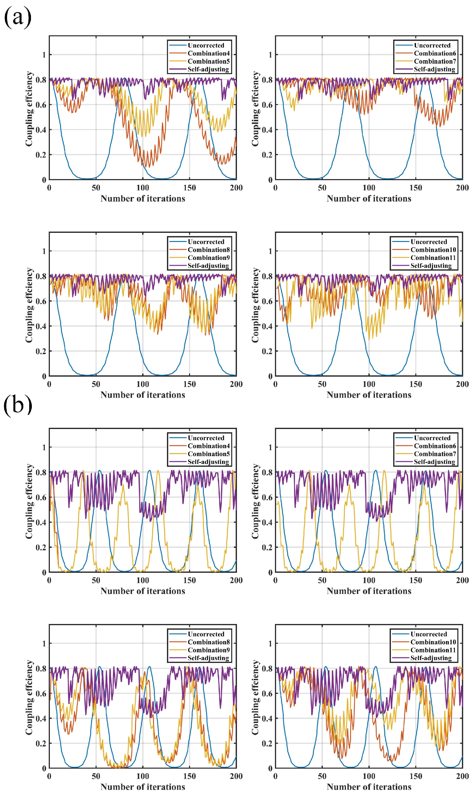
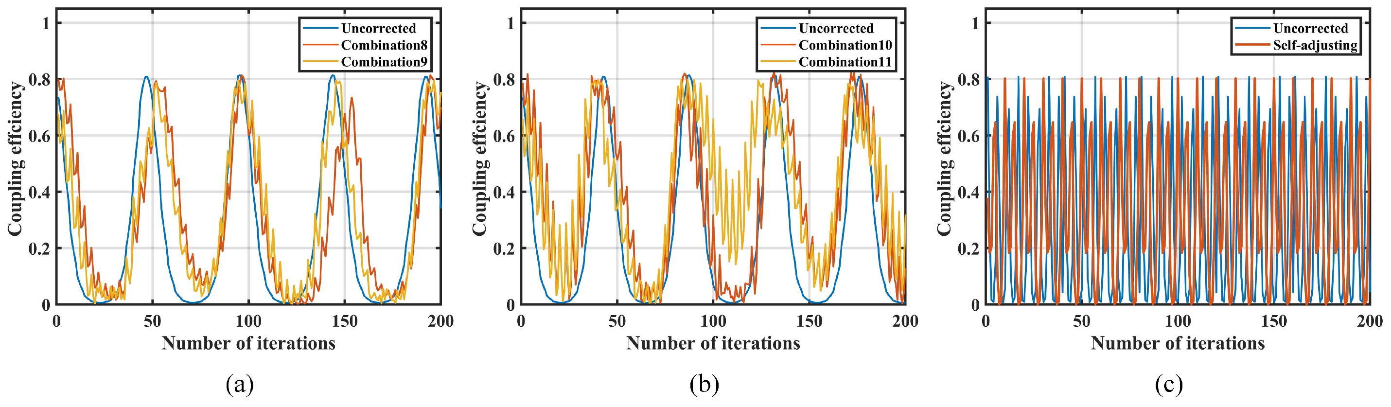
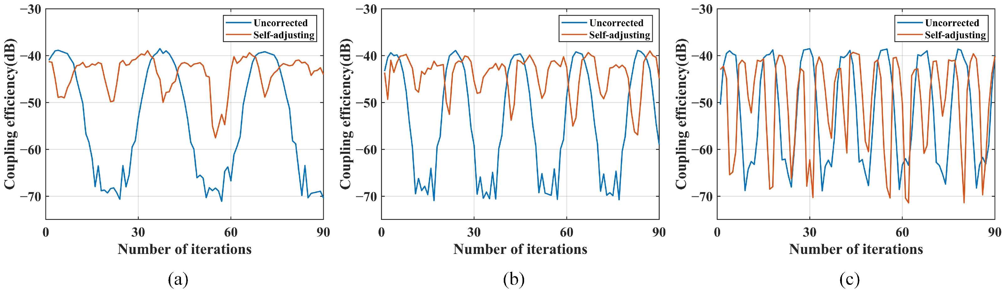
3.2. Dynamic Coupling Experiment of Parameter Self-Adjusting Algorithm
3.3. Summary
4. Conclusions
Author Contributions
Funding
Institutional Review Board Statement
Informed Consent Statement
Data Availability Statement
Conflicts of Interest
References
- Kaushal, H.; Kaddoum, G. Optical communication in space: Challenges and mitigation techniques. IEEE Commun. Surv. Tutor. 2017, 19, 57–96. [Google Scholar] [CrossRef]
- Guiomar, F.P.; Fernandes, M.A.; Nascimento, J.L.; Rodrigues, V.; Monteiro, P.P. Coherent free-space optical communications: Opportunities and challenges. J. Light. Technol. 2022, 40, 3173–3186. [Google Scholar] [CrossRef]
- Kolev, D.R.; Carrasco-Casado, A.; Trinh, P.V.; Shiratama, K.; Ishola, F.; Kotake, H.; Nakazono, J.; Saito, Y.; Kunimori, H.; Kubooka, T.; et al. Latest Developments in the Field of Optical Communications for Small Satellites and Beyond. J. Light. Technol. 2023, 41, 3750–3757. [Google Scholar] [CrossRef]
- Liu, Z.; Gao, S.; Wu, J.; Chen, Y.; Ma, L.; Yu, X.; Wang, X.; Li, R. Research on the NI-MLA Method for Enhancing the Spot Position Detection Accuracy of Quadrant Detectors Under Atmospheric Turbulence. Sensors 2024, 24, 6684. [Google Scholar] [CrossRef]
- Velasco, L.; Ahmadian, M.; Ortiz, L.; Brito, J.P.; Pastor, A.; Rivas, J.M.; Barzegar, S.; Comellas, J.; Martin, V.; Ruiz, M. Scenarios for Optical Encryption Using Quantum Keys. Sensors 2024, 24, 6631. [Google Scholar] [CrossRef]
- Liang, H.; Yi, Z.; Ling, H.; Luo, K. Modeling and Simulation of Inter-Satellite Laser Communication for Space-Based Gravitational Wave Detection. Sensors 2025, 25, 1068. [Google Scholar] [CrossRef] [PubMed]
- Li, Z.; Pan, Z.; Li, Y.; Yang, X.; Geng, C.; Li, X. Advanced root mean square propagation with the warm-up algorithm for fiber coupling. Opt. Express 2023, 3, 23974–23989. [Google Scholar] [CrossRef]
- Dikmelik, Y.; Davidson, F.M. Fiber-coupling efficiency for free-space optical communication through atmospheric turbulence. Appl. Opt. 2005, 44, 4946–4952. [Google Scholar] [CrossRef]
- Zhao, X.; Hou, X.; Zhu, F.; Li, T.; Sun, J.; Zhu, R.; Gao, M.; Yang, Y.; Chen, W. Experimental verification of coherent tracking system based on fiber nutation. Opt. Express 2019, 27, 23996–24006. [Google Scholar] [CrossRef]
- Takenaka, H.; Toyoshima, M.; Takayama, Y. Experimental verification of fiber-coupling efficiency for satellite-to-ground atmospheric laser downlinks. Opt. Express 2012, 20, 15301–15308. [Google Scholar] [CrossRef]
- Lv, F.; Liu, Y.; Gao, S.; Wu, H.; Guo, F. Research on Bandwidth Improvement of Fine Tracking Control System in Space Laser Communication. Photonics 2023, 10, 1179. [Google Scholar] [CrossRef]
- Swanson, E.A.; Bondurant, R.S. Using fiber optics to simplify free-space lasercom systems. Proc. SPIE 1990, 1218, 70–82. [Google Scholar] [CrossRef]
- Hu, Q.; Zhen, L.; Mao, Y.; Zhu, S.; Zhou, X.; Zhou, G. Adaptive stochastic parallel gradient descent approach for efficient fiber coupling. Opt. Express 2020, 28, 13141–13154. [Google Scholar] [CrossRef]
- Bian, Y.; Li, Y.; Chen, E.; Li, W.; Hong, X.; Qiu, J.; Wu, J. Free-space to single-mode fiber coupling efficiency with optical system aberration and fiber positioning error under atmospheric turbulence. J. Opt. 2022, 24, 025703. [Google Scholar] [CrossRef]
- Zhang, L.; Yu, X.; Zhao, B.; Wang, T.; Tong, S. Method for 10 Gbps near-ground quasi-static free-space laser transmission by nutation mutual coupling. Opt. Express 2022, 30, 33465–33478. [Google Scholar] [CrossRef]
- Li, Z.; Pan, Z.; Li, Y.; Yang, X.; Li, F.; Geng, C.; Li, X. Parameter-free fiber coupling method for inter-satellite laser communications based on Gaussian approximation. J. Opt. Commun. Netw. 2024, 16, 258–269. [Google Scholar] [CrossRef]
- Pan, Z.; Li, Z.; Li, Y.; Huang, G.; Zou, F.; Pan, L.; Lin, M.; Li, F.; Geng, C.; Li, X. Experimental demonstration of free-space optical communication under 2 km urban atmosphere using adaptive fiber coupling. Opt. Commun. 2025, 576, 131151. [Google Scholar] [CrossRef]
- Li, B.; Liu, Y.; Tong, S.; Zhang, L.; Yao, H. Adaptive Single-Mode Fiber Coupling Method Based on Coarse-Fine Laser Nutation. IEEE Photonics J. 2018, 10, 1–12. [Google Scholar] [CrossRef]
- Zhu, S.W.; Sheng, L.; Liu, Y.K.; Zhang, Y.; Gao, S. Laser Nutation Coupling Algorithm for Single Mode Fiber Based on Energy Feedback. Chin. J. Lasers 2019, 46, 0206001. [Google Scholar] [CrossRef]
- Toyoshima, M. Maximum fiber coupling efficiency and optimum beam size in the presence of random angular jitter for free-space laser systems and their applications. J. Opt. Soc. Am. A 2006, 23, 2246–2250. [Google Scholar] [CrossRef]
- Chen, B.; Liu, X.P.; Ge, S.S.; Lin, C. Adaptive fuzzy control of a class of nonlinear systems by fuzzy approximation approach. IEEE Trans. Fuzzy Syst. 2012, 20, 1012–1021. [Google Scholar] [CrossRef]
- Labiod, S.; Boucherit, M.S.; Guerra, T.M. Adaptive fuzzy control of a class of MIMO nonlinear systems. Fuzzy Sets Syst. 2005, 151, 59–77. [Google Scholar] [CrossRef]
- Wang, J.; Rad, A.; Chan, P. Indirect adaptive fuzzy sliding mode control: Part I: Fuzzy switching. Fuzzy Sets Syst. 2001, 122, 21–30. [Google Scholar] [CrossRef]
- Passino, K.M.; Yurkovich, S. Fuzzy Control; Addison-Wesley: Boston, MA, USA, 1998; Chapter 2; pp. 60–67. [Google Scholar]
- Zhang, H.; Liu, D. Fuzzy Modeling and Fuzzy Control; Springer Science & Business Media: Berlin/Heidelberg, Germany, 2006; Chapter 1; pp. 9–32. [Google Scholar]
- Cai, X.; Fu, Z.; Xie, H.; Xue, J.; Luo, H.; Ou, N.; Zhou, G. Energy-Feedback Load Simulation Algorithm Based on Fuzzy Control. Appl. Sci. 2022, 12, 5519. [Google Scholar] [CrossRef]
- Chen, Y.-T.; Hsiu, H.; Chen, R.-J.; Chen, P.-N. Stability of virtual reality haptic feedback incorporating fuzzy-passivity control. Meas. Control 2023, 56, 493–506. [Google Scholar] [CrossRef]

| Fixed Parameter | Parameter Value |
|---|---|
| Optical Maser Wavelength | 1550 nm |
| Coupled Lens Equivalent Focal Length | 50 mm |
| Mode Field Diameter | 5.2 μm |
| Diameter | 10 mm |
| Controls Parameter | Pt | P | ||
|---|---|---|---|---|
| S | M | L | ||
| r | S | XL | M | VS |
| L | L | M | S | |
| d | S | XL | M | VS |
| L | L | M | S | |
| n | S | F | F | H |
| L | F | H | H |
| Combined Parameter Selection | Consequence | η | σ | Iterations | ||||
|---|---|---|---|---|---|---|---|---|
| Combination 1 | 0.25 | 0.60 | 4 | Success | 0.678 | 0.0030 | 98 | |
| Combination 2 | 0.2 | 0.50 | 6 | Success | 0.680 | 0.0026 | 114 | |
| Combination 3 | 0.15 | 0.40 | 4 | Success | 0.681 | 0.0016 | 138 | |
| Self-adjusting | Success | 0.683 | 0.00010 | 82 | ||||
| Experimental Group | At 0.5 Hz | At 1.0 Hz | |||||||
|---|---|---|---|---|---|---|---|---|---|
| PV | RMS | σ | PV | RMS | σ | ||||
| Combination 4 | 0.50 | 0.80 | 4 | 0.805 | 0.541 | 0.236 | 0.807 | 0.352 | 0.255 |
| Combination 5 | 0.50 | 1.00 | 6 | 0.469 | 0.669 | 0.137 | 0.807 | 0.347 | 0.252 |
| Combination 6 | 0.60 | 1.20 | 8 | 0.388 | 0.704 | 0.109 | 0.807 | 0.347 | 0.252 |
| Combination 7 | 0.60 | 1.40 | 4 | 0.711 | 0.766 | 0.051 | 0.814 | 0.347 | 0.252 |
| Combination 8 | 0.70 | 1.60 | 6 | 0.614 | 0.650 | 0.151 | 0.814 | 0.407 | 0.263 |
| Combination 9 | 0.70 | 1.80 | 8 | 0.497 | 0.683 | 0.128 | 0.814 | 0.438 | 0.259 |
| Combination 10 | 0.80 | 2.00 | 4 | 0.518 | 0.674 | 0.120 | 0.779 | 0.497 | 0.244 |
| Combination 11 | 0.80 | 2.20 | 4 | 0.525 | 0.687 | 0.123 | 0.711 | 0.565 | 0.199 |
| Self-adjusting | 0.180 | 0.773 | 0.041 | 0.408 | 0.697 | 0.110 | |||
| Parameter Combination | Self-Adjusting | 4 | 5 | 6 | 7 | 8 | 9 | 10 | 11 |
|---|---|---|---|---|---|---|---|---|---|
| Bandwidth/Hz | 10 | 0.8 | 0.8 | 0.9 | 0.9 | 1.1 | 1.1 | 1.2 | 1.2 |
| Initial Position | Coupling Result | Number of Iterations/Times | Steady Accuracy/dBm | |||||||
|---|---|---|---|---|---|---|---|---|---|---|
| Self-Adjusting | Tradition1 | Tradition2 | Self-Adjusting | Tradition1 | Tradition2 | Self-Adjusting | Tradition1 | Tradition2 | ||
| 1 | (0 V, 10 V) | Success | Failure | Failure | 14 | None | None | −36.9 | −54.5 | −53.2 |
| 2 | (2 V, 8 V) | Success | Failure | Failure | 12 | None | None | −36.8 | −54.6 | −53.8 |
| 3 | (3.5 V, 6.5 V) | Success | Success | Success | 8 | 144 | 132 | −36.9 | −37.5 | −37.2 |
| 4 | (3.5 V, 3.5 V) | Success | Success | Success | 8 | 138 | 125 | −37.0 | −37.6 | −37.4 |
| 5 | (5 V, 5 V) | Success | Success | Success | 3 | 68 | 49 | −36.9 | −37.7 | −37.5 |
| 6 | (6.5 V, 6.5 V) | Success | Success | Success | 7 | 136 | 122 | −36.8 | −37.4 | −37.2 |
| 7 | (6.5 V, 3.5 V) | Success | Success | Success | 8 | 154 | 141 | −37.0 | −37.6 | −37.4 |
| 8 | (8 V, 2 V) | Success | Failure | Failure | 11 | None | None | −36.7 | −54.8 | −53.6 |
| 9 | (10 V, 0 V) | Success | Failure | Failure | 14 | None | None | −36.9 | −55.2 | −54.4 |
Disclaimer/Publisher’s Note: The statements, opinions and data contained in all publications are solely those of the individual author(s) and contributor(s) and not of MDPI and/or the editor(s). MDPI and/or the editor(s) disclaim responsibility for any injury to people or property resulting from any ideas, methods, instructions or products referred to in the content. |
© 2025 by the authors. Licensee MDPI, Basel, Switzerland. This article is an open access article distributed under the terms and conditions of the Creative Commons Attribution (CC BY) license (https://creativecommons.org/licenses/by/4.0/).
Share and Cite
Liu, Y.; Li, S.; Lv, F.; Wang, X.; Chen, B.; Guo, C.; Yao, K.; Wang, J. Parameter Self-Adjusting Single-Mode Fiber Nutation Coupling Algorithm Based on Fuzzy Control. Sensors 2025, 25, 3051. https://doi.org/10.3390/s25103051
Liu Y, Li S, Lv F, Wang X, Chen B, Guo C, Yao K, Wang J. Parameter Self-Adjusting Single-Mode Fiber Nutation Coupling Algorithm Based on Fuzzy Control. Sensors. 2025; 25(10):3051. https://doi.org/10.3390/s25103051
Chicago/Turabian StyleLiu, Yongkai, Shuqiang Li, Furui Lv, Ximing Wang, Baogang Chen, Chenzi Guo, Kainan Yao, and Jianli Wang. 2025. "Parameter Self-Adjusting Single-Mode Fiber Nutation Coupling Algorithm Based on Fuzzy Control" Sensors 25, no. 10: 3051. https://doi.org/10.3390/s25103051
APA StyleLiu, Y., Li, S., Lv, F., Wang, X., Chen, B., Guo, C., Yao, K., & Wang, J. (2025). Parameter Self-Adjusting Single-Mode Fiber Nutation Coupling Algorithm Based on Fuzzy Control. Sensors, 25(10), 3051. https://doi.org/10.3390/s25103051