

Time-Frequency Analysis of Motor Imagery During Plantar and Dorsal Flexion Movements Using a Low-Cost Ankle Exoskeleton
 ,
,  , ,
, ,  and
and 
Abstract
1. Introduction
2. Materials and Methods
2.1. Materials
2.1.1. Subjects
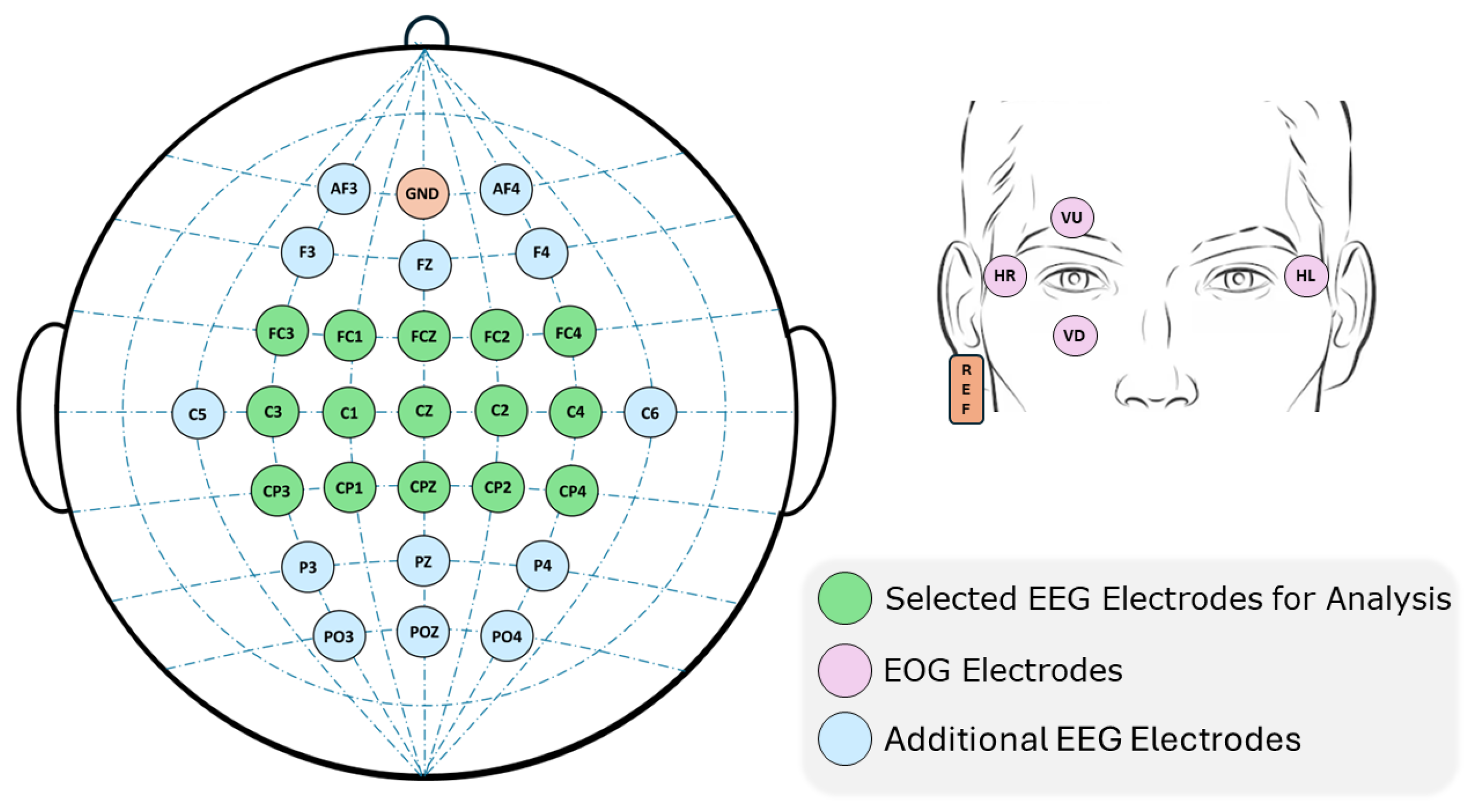
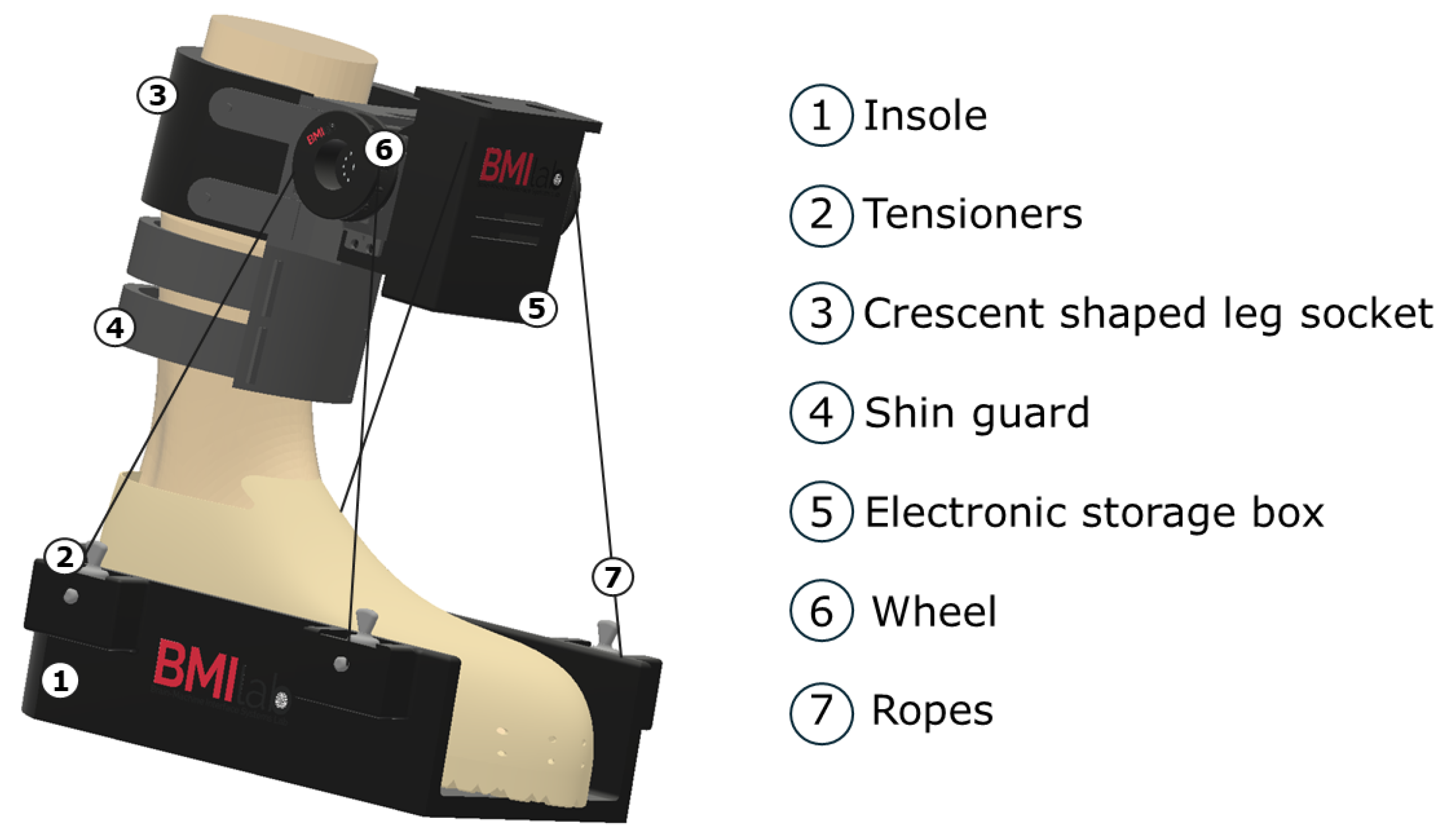
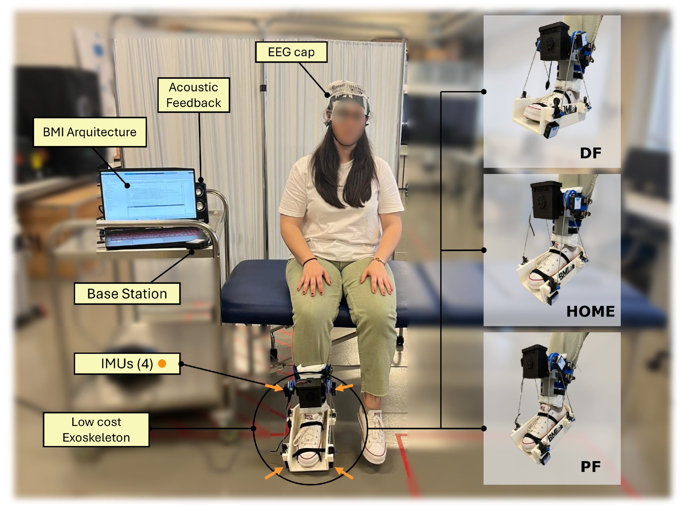
2.1.2. Equipment
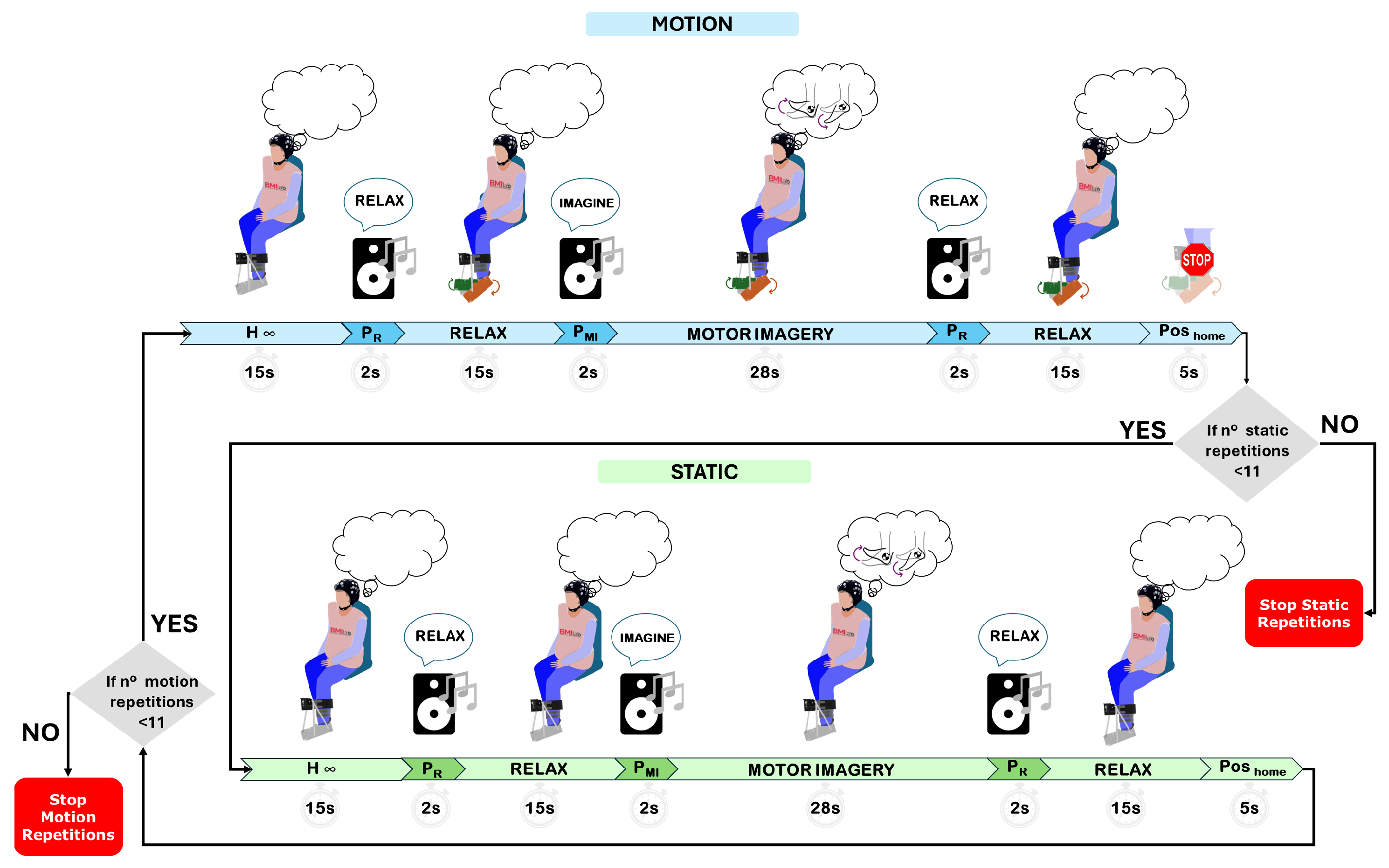
2.1.3. Experimental Protocol
2.2. Methods
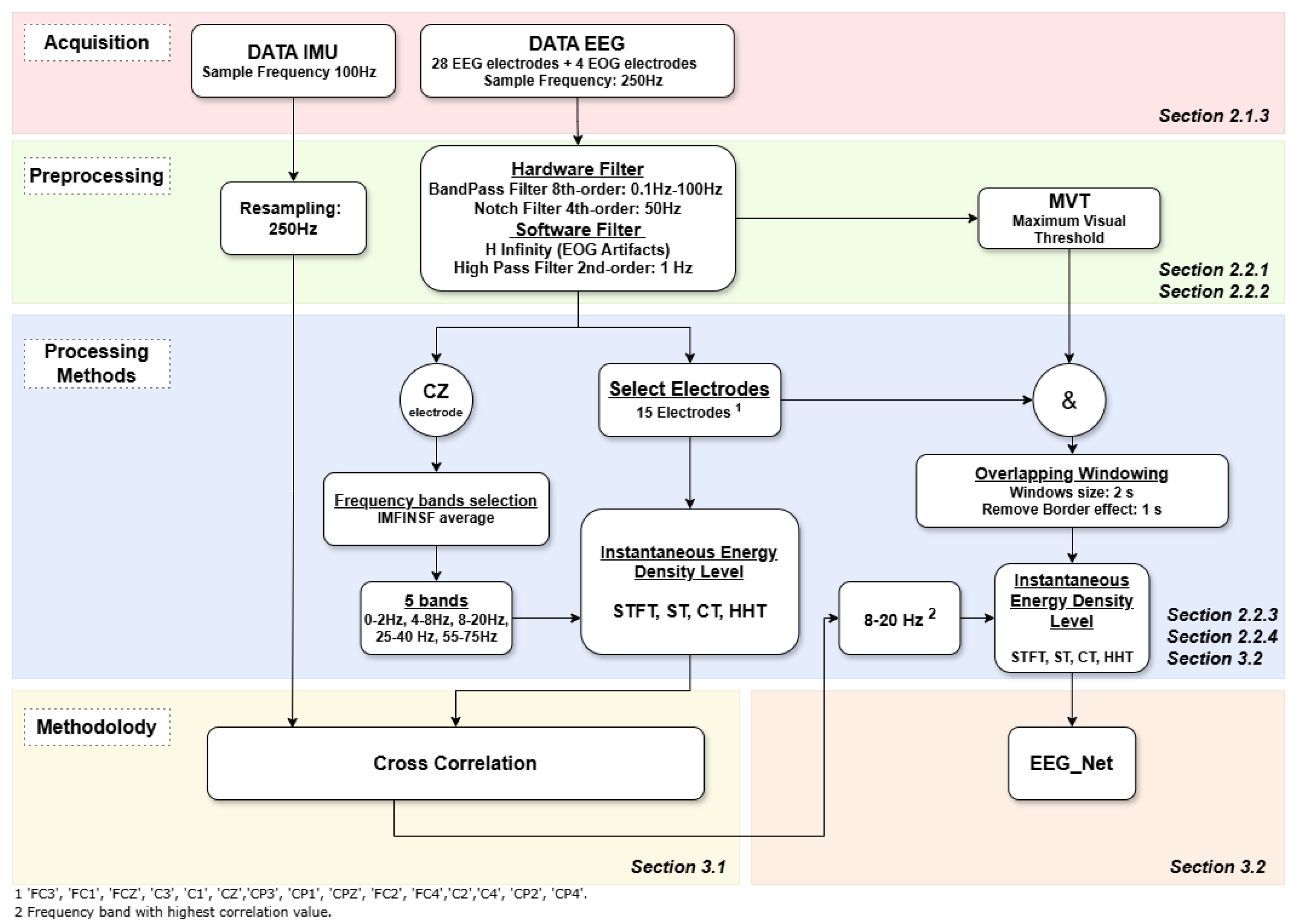
2.2.1. Signal Preprocessing
2.2.2. Normalize Data for Motor Imagery Decoding Analysis
2.2.3. Data Analysis
Short-Time Fourier Transform
Stockwell Transform
Hilbert–Huang Transform with VMD
Chirplet Transform
2.2.4. Frequency Bands Selection
2.2.5. Statistical Analysis
3. Methodology
3.1. Correlation Analysis of Motion Trials
3.2. Motor Imagery Decoding
4. Results
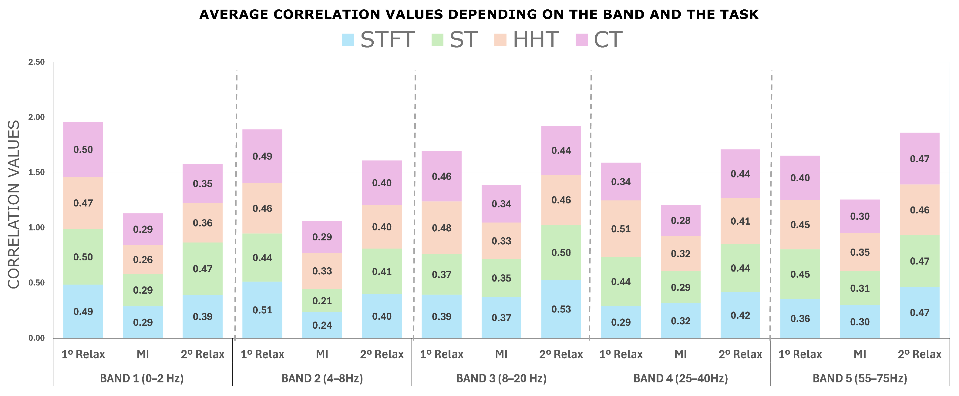
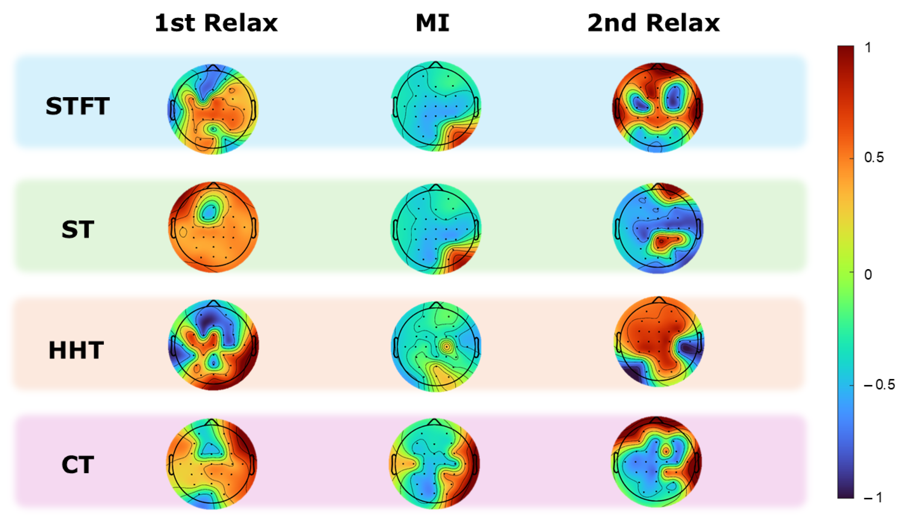
4.1. Motion Correlation Results
- Average correlation per band and mental task.
- Correlation per electrode
- Differences between mental tasks
- Differences between transforms
- Lag analysis
Statistical Analysis of Correlation Results
4.2. Motor Imagery Decoding Results
Statistical Analysis of Motor Imagery Decoding Results
5. Discussion
6. Limitations
7. Conclusions
Author Contributions
Funding
Institutional Review Board Statement
Informed Consent Statement
Data Availability Statement
Conflicts of Interest
References
- He, Y.; Eguren, D.; Azorín, J.M.; Grossman, R.G.; Luu, T.P.; Contreras-Vidal, J.L. Brain-machine interfaces for controlling lower-limb powered robotic systems. J. Neural Eng. 2018, 15, 021004. [Google Scholar] [CrossRef] [PubMed]
- King, C.E.; Wang, P.T.; Chui, L.A.; Do, A.H.; Nenadic, Z. Operation of a brain-computer interface walking simulator for individuals with spinal cord injury. J. Neuroeng. Rehabil. 2013, 10, 77. [Google Scholar] [CrossRef]
- Yang, H.; Guan, C.; Wang, C.C.; Ang, K.K. Detection of motor imagery of brisk walking from electroencephalogram. J. Neurosci. Methods 2015, 244, 33–44. [Google Scholar] [CrossRef] [PubMed]
- Ferrero, L.; Ortiz, M.; Quiles, V.; Iáñez, E.; Flores, J.A.; Azorín, J.M. Brain symmetry analysis during the use of a BCI based on motor imagery for the control of a lower-limb exoskeleton. Symmetry 2021, 13, 1746. [Google Scholar] [CrossRef]
- Shyam, A.K.B.; Wadhwani. Investigation of the Impact of EEG Signal Processing Techniques on Classification Performance. In Proceedings of the Machine Vision and Augmented Intelligence, Patna, India, 24–25 November 2023; Kumar Singh, K., Singh, S., Srivastava, S., Bajpai, M.K., Eds.; Springer Nature: Singapore, 2023; pp. 265–283. [Google Scholar]
- Pup, F.D.; Zanola, A.; Tshimanga, L.F.; Bertoldo, A.; Atzori, M. The More, the Better? Evaluating the Role of EEG Preprocessing for Deep Learning Applications. IEEE Trans. Neural Syst. Rehabil. Eng. 2025, 33, 1061–1070. [Google Scholar] [CrossRef] [PubMed]
- Jiang, X.; Bian, G.B.; Tian, Z. Removal of artifacts from EEG signals: A review. Sensors 2019, 19, 987. [Google Scholar] [CrossRef]
- Ramoser, H.; Müller-Gerking, J.; Pfurtscheller, G. Optimal spatial filtering of single trial EEG during imagined hand movement. IEEE Trans. Rehabil. Eng. 2000, 8, 441–446. [Google Scholar] [CrossRef]
- Herman, P.; Prasad, G.; McGinnity, T.M.; Coyle, D. Comparative analysis of spectral approaches to feature extraction for EEG-based motor imagery classification. IEEE Trans. Neural Syst. Rehabil. Eng. 2008, 16, 317–326. [Google Scholar] [CrossRef]
- Morales, S.; Bowers, M.E. Time-frequency analysis methods and their application in developmental EEG data. Dev. Cogn. Neurosci. 2022, 54, 101067. [Google Scholar] [CrossRef]
- Zhang, L.; Wu, D.; Zhi, L. Method of removing noise from EEG signals based on HHT method. In Proceedings of the 2009 1st International Conference on Information Science and Engineering, ICISE 2009, Nanjing, China, 26–28 December 2009. [Google Scholar] [CrossRef]
- Jindal, K.; Upadhyay, R.; Singh, H.S. Application of hybrid GLCT-PICA de-noising method in automated EEG artifact removal. Biomed. Signal Process. Control 2020, 60, 101977. [Google Scholar] [CrossRef]
- Bhargava, A.; Mann, S. Adaptive Chirplet Transform-Based Machine Learning for P300 Brainwave Classification. In Proceedings of the Proceedings—2020 IEEE EMBS Conference on Biomedical Engineering and Sciences, IECBES 2020, Langkawi Island, Malaysia, 1–3 March 2021. [Google Scholar] [CrossRef]
- Jiang, Y.; Chen, W.; Li, M.; Zhang, T.; You, Y. Synchroextracting chirplet transform-based epileptic seizures detection using EEG. Biomed. Signal Process. Control 2021, 68, 102699. [Google Scholar] [CrossRef]
- Kaur, M.; Upadhyay, R.; Kumar, V. A Hybrid Deep Learning Framework Using Scaling-Basis Chirplet Transform for Motor Imagery EEG Recognition in Brain–Computer Interface Applications. Int. J. Imaging Syst. Technol. 2024, 34, e23127. [Google Scholar] [CrossRef]
- Kalbkhani, H.; Shayesteh, M.G. Stockwell transform for epileptic seizure detection from EEG signals. Biomed. Signal Process. Control 2017, 38, 108–118. [Google Scholar] [CrossRef]
- Ortiz, M.; Rodríguez-Ugarte, M.; Iáñez, E.; Azorín, J.M. Application of the stockwell transform to electroencephalographic signal analysis during gait cycle. Front. Neurosci. 2017, 11, 660. [Google Scholar] [CrossRef]
- Ortiz, M.; Ferrero, L.; Iáñez, E.; Azorín, J.M.; Contreras-Vidal, J.L. Sensory Integration in Human Movement: A New Brain-Machine Interface Based on Gamma Band and Attention Level for Controlling a Lower-Limb Exoskeleton. Front. Bioeng. Biotechnol. 2020, 8, 735. [Google Scholar] [CrossRef]
- Salimpour, S.; Kalbkhani, H.; Seyyedi, S.; Solouk, V. Stockwell transform and semi-supervised feature selection from deep features for classification of BCI signals. Sci. Rep. 2022, 12, 11773. [Google Scholar] [CrossRef]
- Sethi, S.; Upadhyay, R.; Singh, H.S. Stockwell-common spatial pattern technique for motor imagery-based Brain Computer Interface design. Comput. Electr. Eng. 2018, 71, 492–504. [Google Scholar] [CrossRef]
- Wang, L.; Xu, G.; Wang, J.; Yang, S.; Yan, W. Application of Hilbert-Huang transform for the study of motor imagery tasks. In Proceedings of the 30th Annual International Conference of the IEEE Engineering in Medicine and Biology Society, Vancouver, BC, Canada, 20–25 August 2008. [Google Scholar] [CrossRef]
- Yu, Y.; Zhao, Y.; Li, S.; Shi, L.; Li, Z.; Dong, B. Motor imagery EEG discrimination using Hilbert-Huang Entropy. Biomed. Res. 2017, 28, 727–733. [Google Scholar]
- Ortiz, M.; Iáñez, E.; Contreras-Vidal, J.L.; Azorín, J.M. Analysis of the EEG Rhythms Based on the Empirical Mode Decomposition During Motor Imagery When Using a Lower-Limb Exoskeleton. A Case Study. Front. Neurorobot. 2020, 14, 48. [Google Scholar] [CrossRef]
- Kim, H.; Yoshimura, N.; Koike, Y. Characteristics of Kinematic Parameters in Decoding Intended Reaching Movements Using Electroencephalography (EEG). Front. Neurosci. 2019, 13, 1148. [Google Scholar] [CrossRef]
- Lv, J.; Li, Y.; Gu, Z. Decoding hand movement velocity from electroencephalogram signals during a drawing task. BioMed Eng. Online 2010, 9, 64. [Google Scholar] [CrossRef] [PubMed]
- Robinson, N.; Guan, C.; Vinod, A.P. Adaptive estimation of hand movement trajectory in an EEG based brain-computer interface system. J. Neural Eng. 2015, 12, 66019. [Google Scholar] [CrossRef] [PubMed]
- Meier, J.D.; Aflalo, T.N.; Kastner, S.; Graziano, M.S. Complex organization of human primary motor cortex: A high-resolution fMRI study. J. Neurophysiol. 2008, 100, 1800–1812. [Google Scholar] [CrossRef]
- Tobar, A.M.; Hyoudou, R.; Kita, K.; Nakamura, T.; Kambara, H.; Ogata, Y.; Hanakawa, T.; Koike, Y.; Yoshimura, N. Decoding of ankle flexion and extension from cortical current sources estimated from non-invasive brain activity recording methods. Front. Neurosci. 2018, 11, 733. [Google Scholar] [CrossRef]
- O’Keeffe, R.; Shirazi, S.Y.; Vecchio, A.D.; Ibanez, J.; Mrachacz-Kersting, N.; Bighamian, R.; Rizzo, J.; Farina, D.; Atashzar, S.F. Low-frequency motor cortex EEG predicts four levels of rate of change of force during ankle dorsiflexion. bioRxiv 2022. [Google Scholar] [CrossRef]
- Jiang, N.; Gizzi, L.; Mrachacz-Kersting, N.; Dremstrup, K.; Farina, D. A brain-computer interface for single-trial detection of gait initiation from movement related cortical potentials. Clin. Neurophysiol. 2015, 126, 154–159. [Google Scholar] [CrossRef] [PubMed]
- Donati, A.R.; Shokur, S.; Morya, E.; Campos, D.S.; Moioli, R.C.; Gitti, C.M.; Augusto, P.B.; Tripodi, S.; Pires, C.G.; Pereira, G.A.; et al. Long-Term Training with a Brain-Machine Interface-Based Gait Protocol Induces Partial Neurological Recovery in Paraplegic Patients. Sci. Rep. 2016, 6, 30383. [Google Scholar] [CrossRef]
- Pinto, D.; Garnier, M.; Barbas, J.; Chang, S.H.; Charlifue, S.; Field-Fote, E.; Furbish, C.; Tefertiller, C.; Mummidisetty, C.K.; Taylor, H.; et al. Budget impact analysis of robotic exoskeleton use for locomotor training following spinal cord injury in four SCI Model Systems. J. Neuroeng. Rehabil. 2020, 17, 4. [Google Scholar] [CrossRef] [PubMed]
- Collins, S.H.; Wiggin, M.B.; Sawicki, G.S. Reducing the energy cost of human walking using an unpowered exoskeleton. Nature 2015, 522, 212–215. [Google Scholar] [CrossRef]
- Trapero-Asenjo, S.; Gallego-Izquierdo, T.; Pecos-Martín, D.; Nunez-Nagy, S. Translation, cultural adaptation, and validation of the Spanish version of the Movement Imagery Questionnaire-3 (MIQ-3). Musculoskelet. Sci. Pract. 2021, 51, 102313. [Google Scholar] [CrossRef]
- g.tec Medical Engineering GmbH. g.Nautilus PRO FLEXIBLE–Wireless EEG/ECG/EMG System. 2025. Available online: https://www.gtec.at/product/g-nautilus-pro-flexible (accessed on 14 April 2025).
- WIT Motion. WT901BLECL BLE 9-Axis High-Precision Attitude Sensor IMU. 2025. Available online: https://www.wit-motion.com/BLE/52.html (accessed on 14 April 2025).
- Ferrero, L.; Quiles, V.; Ortiz, M.; Iáñez, E.; Azorín, J.M. A BMI based on motor imagery and attention for commanding a lower-limb robotic exoskeleton: A case study. Appl. Sci. 2021, 11, 4106. [Google Scholar] [CrossRef]
- Kilicarslan, A.; Grossman, R.G.; Contreras-Vidal, J.L. A robust adaptive denoising framework for real-time artifact removal in scalp EEG measurements. J. Neural Eng. 2016, 13, 26013. [Google Scholar] [CrossRef]
- Goldberg, G. Supplementary motor area structure and function: Review and hypotheses. Behav. Brain Sci. 1985, 8, 567–588. [Google Scholar] [CrossRef]
- Boehme, T.K.; Bracewell, R. The Fourier Transform and its Applications. Am. Math. Mon. 1966, 73, 27–34. [Google Scholar] [CrossRef]
- Huang, N.E.; Shen, Z.; Long, S.R.; Wu, M.C.; Shih, H.H.; chyuan Yen, N.; Tung, C.C.; Liu, H.H. The empirical mode decomposition and the Hilbert spectrum for nonlinear and non-stationary time series analysis. Proc. R. Soc. A 1996, 454, 903–995. [Google Scholar] [CrossRef]
- Stockwell, R.G.; Mansinha, L.; Lowe, R.P. Localization of the complex spectrum: The S transform. IEEE Trans. Signal Process. 1996, 44, 998–1001. [Google Scholar] [CrossRef]
- Mann, S.; Haykin, S. The Chirplet Transform: Physical Considerations. IEEE Trans. Signal Process. 1995, 43, 2745–2761. [Google Scholar] [CrossRef] [PubMed]
- Fu, K.; Qu, J.; Chai, Y.; Zou, T. Hilbert marginal spectrum analysis for automatic seizure detection in EEG signals. Biomed. Signal Process. Control 2015, 18, 179–185. [Google Scholar] [CrossRef]
- Dragomiretskiy, K.; Zosso, D. Variational mode decomposition. IEEE Trans. Signal Process. 2014, 62, 531–544. [Google Scholar] [CrossRef]
- Peng, Z.K.; Meng, G.; Chu, F.L.; Lang, Z.Q.; Zhang, W.M.; Yang, Y. Polynomial chirplet transform with application to instantaneous frequency estimation. IEEE Trans. Instrum. Meas. 2011, 60, 3222–3229. [Google Scholar] [CrossRef]
- Delgado, A.L.; Delisle-Rodriguez, D.; da Rocha, A.F.; Figueroa, E.S.; López-Delis, A. Revisión sobre nuevos enfoques de terapias de neurorrehabilitación para pacientes con trastornos neurológicos mediante dispositivos de pedaleo. Neurol. Argent. 2024, 16, 31–43. [Google Scholar] [CrossRef]
- Sugumar, D.; Vanathi, P.T. EEG Signal Separation using Improved EEMD-Fast IVA Algorithm. Asian J. Res. Soc. Sci. Humanit. 2017, 7, 1230–1243. [Google Scholar] [CrossRef]
- Field, A. Discovering Statistics Using SPSS Statistics; Sage Publications: Los Angeles, LA, USA, 2013. [Google Scholar]
- Box, G.E.P.; Jenkins, G.M.; Reinsel, G.C. Time Series Analysis: Forecasting and Control, 3rd ed.; Prentice Hall: Englewood Cliffs, NJ, USA, 1994. [Google Scholar]
- Lawhern, V.J.; Solon, A.J.; Waytowich, N.R.; Gordon, S.M.; Hung, C.P.; Lance, B.J. EEGNet: A compact convolutional neural network for EEG-based brain-computer interfaces. J. Neural Eng. 2018, 15, 056013. [Google Scholar] [CrossRef] [PubMed]
- Loshchilov, I.; Hutter, F. SGDR: Stochastic gradient descent with warm restarts. In Proceedings of the 5th International Conference on Learning Representations, ICLR 2017-Conference Track Proceedings, Toulon, France, 24–26 April 2017. [Google Scholar]
- Pfurtscheller, G.; Neuper, C. Motor imagery activates primary sensorimotor area in humans. Neurosci. Lett. 1997, 239, 65–68. [Google Scholar] [CrossRef] [PubMed]
- Friedman, M. The use of ranks to avoid the assumption of normality implicit in the analysis of variance. J. Am. Stat. Assoc. 1937, 32, 675–701. [Google Scholar] [CrossRef]
- Wilcoxon, F. Individual comparisons by ranking methods. Biometrics 1945, 1, 80–83. [Google Scholar] [CrossRef]
- Kruskal, W.H.; Wallis, W.A. Use of ranks in one-criterion variance analysis. J. Am. Stat. Assoc. 1952, 47, 583–621. [Google Scholar] [CrossRef]
- Jeon, Y.; Nam, C.S.; Kim, Y.J.; Whang, M.C. Event-related (De)synchronization (ERD/ERS) during motor imagery tasks: Implications for brain-computer interfaces. Int. J. Ind. Ergon. 2011, 41, 428–436. [Google Scholar] [CrossRef]
- Nakayashiki, K.; Saeki, M.; Takata, Y.; Hayashi, Y.; Kondo, T. Modulation of event-related desynchronization during kinematic and kinetic hand movements. J. Neuroeng. Rehabil. 2014, 11, 90. [Google Scholar] [CrossRef]
- Pfurtscheller, G.; Brunner, C.; Schlögl, A.; da Silva, F.H.L. Mu rhythm (de)synchronization and EEG single-trial classification of different motor imagery tasks. NeuroImage 2006, 31, 153–159. [Google Scholar] [CrossRef]
- Severens, M.; Nienhuis, B.; Desain, P.; Duysens, J. Feasibility of measuring event Related Desynchronization with electroencephalography during walking. In Proceedings of the Annual International Conference of the IEEE Engineering in Medicine and Biology Society, EMBS, San Diego, CA, USA, 28 August–1 September 2012. [Google Scholar] [CrossRef]
- Wagner, J.; Solis-Escalante, T.; Grieshofer, P.; Neuper, C.; Müller-Putz, G.; Scherer, R. Level of participation in robotic-assisted treadmill walking modulates midline sensorimotor EEG rhythms in able-bodied subjects. NeuroImage 2012, 63, 1203–1211. [Google Scholar] [CrossRef] [PubMed]
- Polo-Hortigüela, C.; Juan, J.V.; Ortiz, M.; Iañez, E.; Azorín, J.M. Análisis de señales EEG en movimientos de flexión plantar y dorsal mediante el empleo de un exoesqueleto de bajo coste para la caracterización de la acción motora. In Proceedings of the XLI Congreso Anual de la Sociedad Española de Ingeniería Biomédica, Cartagena, Colombia, 22–24 November 2023; pp. 381–384. [Google Scholar]
- Hooda, N.; Das, R.; Kumar, N. Fusion of EEG and EMG signals for classification of unilateral foot movements. Biomed. Signal Process. Control 2020, 60, 101990. [Google Scholar] [CrossRef]
- Wierzgała, P.; Zapała, D.; Wojcik, G.M.; Masiak, J. Most popular signal processing methods in motor-imagery BCI: A review and meta-analysis. Front. Neuroinform. 2018, 12, 78. [Google Scholar] [CrossRef] [PubMed]


| Motion (Hz) | 0.59 ± 0.15 | 6.07 ± 1.04 | 15.23 ± 2.78 | 32.20 ± 4.64 | 64.42 ± 7.83 |
| Static (Hz) | 0.57 ± 0.12 | 5.67 ± 0.51 | 14.18 ± 1.97 | 30.26 ± 4.24 | 63.36 ± 9.29 |
| 0–2 Hz | 4–8 Hz | 8–20 Hz | 25–40 Hz | 55–75 Hz |
| Motion | Static | ||||||
|---|---|---|---|---|---|---|---|
| Transform | Subject | ACC Relax | ACC MI | Average | ACC Relax | ACC MI | Average |
| Short-Time Fourier Transform | S1 | 0.90 ± 0.11 | 0.92 ± 0.06 | 0.91 ± 0.07 | 0.79 ± 0.18 | 0.93 ± 0.07 | 0.86 ± 0.09 |
| S2 | 0.94 ± 0.04 | 0.94 ± 0.04 | 0.94 ± 0.02 | 0.95 ± 0.05 | 0.96 ± 0.03 | 0.95 ± 0.02 | |
| S3 | 0.91 ± 0.08 | 0.94 ± 0.13 | 0.92 ± 0.09 | 0.88 ± 0.08 | 0.93 ± 0.06 | 0.90 ± 0.06 | |
| S4 | 0.97 ± 0.03 | 0.97 ± 0.03 | 0.97 ± 0.03 | 0.97 ± 0.03 | 0.90 ± 0.05 | 0.89 ± 0.04 | |
| S5 | 0.92 ± 0.08 | 0.94 ± 0.06 | 0.93 ± 0.06 | 0.87 ± 0.09 | 0.90 ± 0.05 | 0.89 ± 0.04 | |
| S6 | 0.96 ± 0.03 | 0.94 ± 0.03 | 0.96 ± 0.02 | 0.96 ± 0.05 | 0.90 ± 0.09 | 0.95 ± 0.06 | |
| Stockwell Transform | S1 | 0.87 ± 0.12 | 0.87 ± 0.07 | 0.87 ± 0.07 | 0.84 ± 0.13 | 0.87 ± 0.08 | 0.85 ± 0.09 |
| S2 | 0.92 ± 0.05 | 0.89 ± 0.05 | 0.90 ± 0.03 | 0.91 ± 0.07 | 0.92 ± 0.05 | 0.92 ± 0.03 | |
| S3 | 0.89 ± 0.09 | 0.94 ± 0.02 | 0.91 ± 0.05 | 0.83 ± 0.13 | 0.91 ± 0.06 | 0.87 ± 0.08 | |
| S4 | 0.94 ± 0.03 | 0.93 ± 0.05 | 0.93 ± 0.03 | 0.93 ± 0.04 | 0.93 ± 0.04 | 0.93 ± 0.03 | |
| S5 | 0.73 ± 0.11 | 0.88 ± 0.09 | 0.81 ± 0.06 | 0.85 ± 0.10 | 0.81 ± 0.08 | 0.83 ± 0.06 | |
| S6 | 0.93 ± 0.04 | 0.88 ± 0.03 | 0.93 ± 0.02 | 0.92 ± 0.05 | 0.81 ± 0.10 | 0.91 ± 0.06 | |
| Hilbert-Huang | S1 | 0.66 ± 0.14 | 0.67 ± 0.15 | 0.66 ± 0.05 | 0.70 ± 0.07 | 0.60 ± 0.07 | 0.65 ± 0.03 |
| S2 | 0.79 ± 0.10 | 0.75 ± 0.08 | 0.77 ± 0.05 | 0.77 ± 0.08 | 0.78 ± 0.10 | 0.77 ± 0.04 | |
| S3 | 0.90 ± 0.09 | 0.95 ± 0.08 | 0.92 ± 0.08 | 0.60 ± 0.69 | 0.74 ± 0.11 | 0.67 ± 0.04 | |
| S4 | 0.67 ± 0.10 | 0.77 ± 0.08 | 0.72 ± 0.05 | 0.68 ± 0.11 | 0.81 ± 0.07 | 0.75 ± 0.04 | |
| S5 | 0.65 ± 0.17 | 0.72 ± 0.13 | 0.68 ± 0.06 | 0.57 ± 0.12 | 0.69 ± 0.12 | 0.63 ± 0.04 | |
| S6 | 0.65 ± 0.10 | 0.72 ± 0.10 | 0.64 ± 0.04 | 0.64 ± 0.09 | 0.69 ± 0.07 | 0.67 ± 0.05 | |
| Chirplet Transform | S1 | 0.90 ± 0.06 | 0.88 ± 0.13 | 0.89 ± 0.08 | 0.85 ± 0.10 | 0.90 ± 0.08 | 0.88 ± 0.07 |
| S2 | 0.89 ± 0.04 | 0.92 ± 0.06 | 0.90 ± 0.03 | 0.98 ± 0.04 | 0.93 ± 0.04 | 0.95 ± 0.03 | |
| S3 | 0.90 ± 0.09 | 0.89 ± 0.12 | 0.90 ± 0.10 | 0.88 ± 0.09 | 0.88 ± 0.08 | 0.88 ± 0.07 | |
| S4 | 0.94 ± 0.03 | 0.96 ± 0.03 | 0.95 ± 0.02 | 0.92 ± 0.04 | 0.97 ± 0.03 | 0.94 ± 0.03 | |
| S5 | 0.90 ± 0.07 | 0.90 ± 0.06 | 0.90 ± 0.05 | 0.84 ± 0.13 | 0.79 ± 0.09 | 0.82 ± 0.05 | |
| S6 | 0.96 ± 0.02 | 0.90 ± 0.04 | 0.95 ± 0.02 | 0.94 ± 0.09 | 0.92 ± 0.09 | 0.93 ± 0.09 | |
Disclaimer/Publisher’s Note: The statements, opinions and data contained in all publications are solely those of the individual author(s) and contributor(s) and not of MDPI and/or the editor(s). MDPI and/or the editor(s) disclaim responsibility for any injury to people or property resulting from any ideas, methods, instructions or products referred to in the content. |
© 2025 by the authors. Licensee MDPI, Basel, Switzerland. This article is an open access article distributed under the terms and conditions of the Creative Commons Attribution (CC BY) license (https://creativecommons.org/licenses/by/4.0/).
Share and Cite
Polo-Hortigüela, C.; Ortiz, M.; Soriano-Segura, P.; Iáñez, E.; Azorín, J.M. Time-Frequency Analysis of Motor Imagery During Plantar and Dorsal Flexion Movements Using a Low-Cost Ankle Exoskeleton. Sensors 2025, 25, 2987. https://doi.org/10.3390/s25102987
Polo-Hortigüela C, Ortiz M, Soriano-Segura P, Iáñez E, Azorín JM. Time-Frequency Analysis of Motor Imagery During Plantar and Dorsal Flexion Movements Using a Low-Cost Ankle Exoskeleton. Sensors. 2025; 25(10):2987. https://doi.org/10.3390/s25102987
Chicago/Turabian StylePolo-Hortigüela, Cristina, Mario Ortiz, Paula Soriano-Segura, Eduardo Iáñez, and José M. Azorín. 2025. "Time-Frequency Analysis of Motor Imagery During Plantar and Dorsal Flexion Movements Using a Low-Cost Ankle Exoskeleton" Sensors 25, no. 10: 2987. https://doi.org/10.3390/s25102987
APA StylePolo-Hortigüela, C., Ortiz, M., Soriano-Segura, P., Iáñez, E., & Azorín, J. M. (2025). Time-Frequency Analysis of Motor Imagery During Plantar and Dorsal Flexion Movements Using a Low-Cost Ankle Exoskeleton. Sensors, 25(10), 2987. https://doi.org/10.3390/s25102987