

Using Infrared Raman Spectroscopy with Machine Learning and Deep Learning as an Automatic Textile-Sorting Technology for Waste Textiles


Abstract
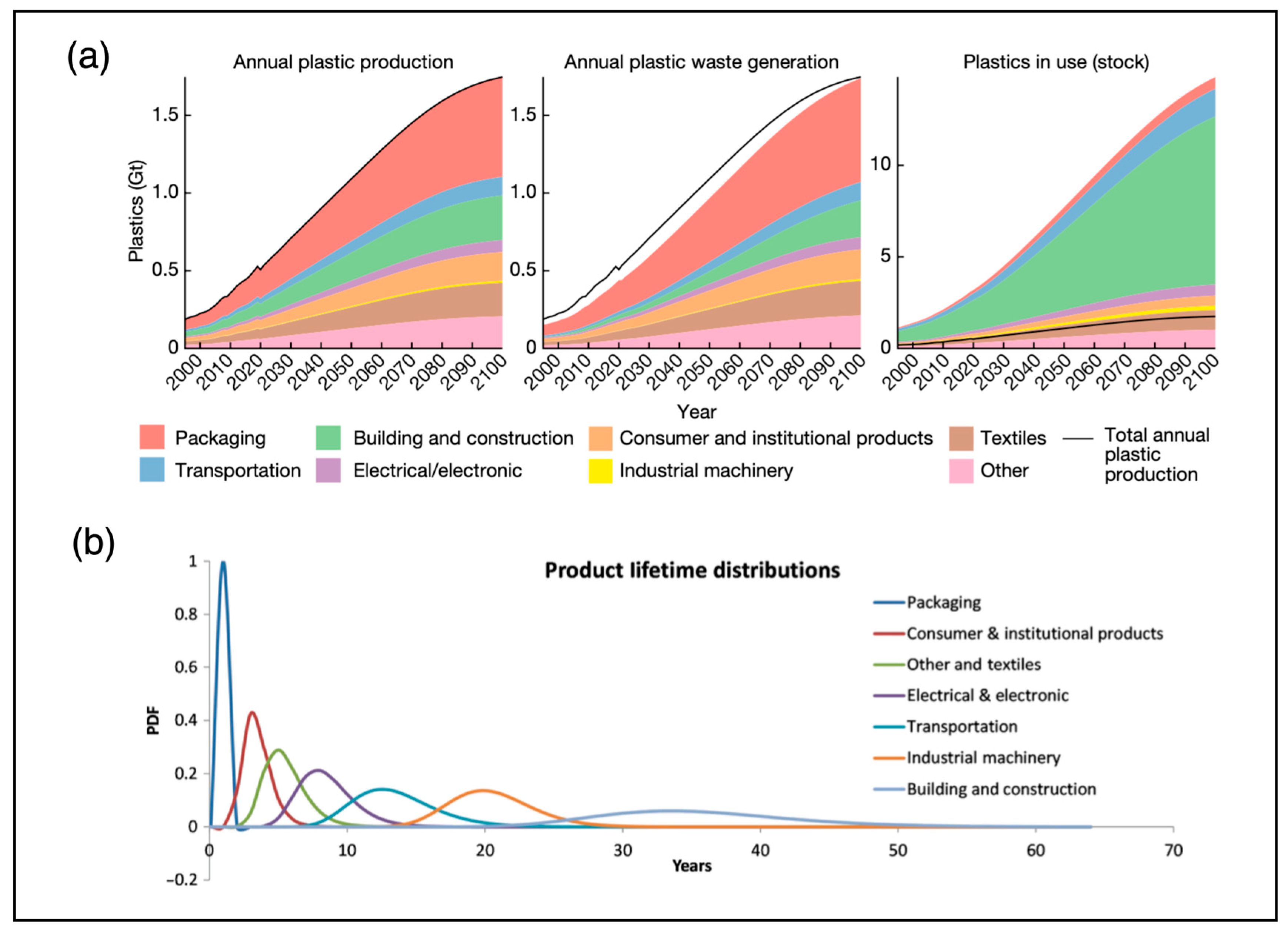
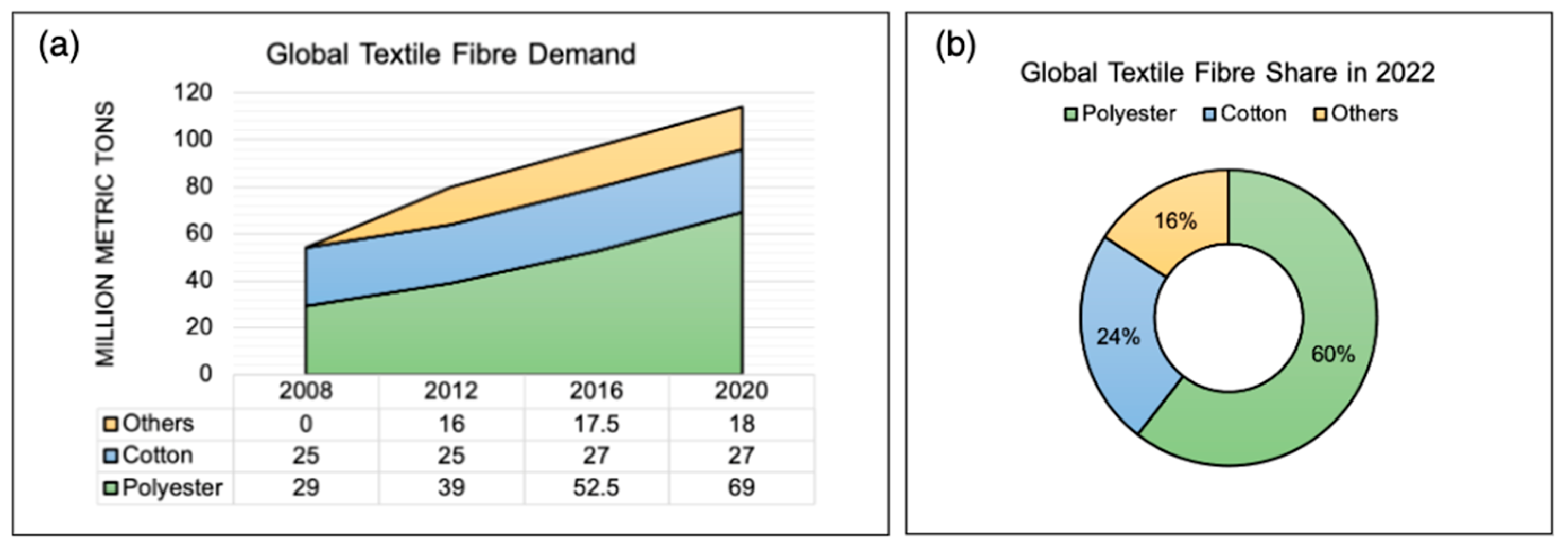
1. Introduction
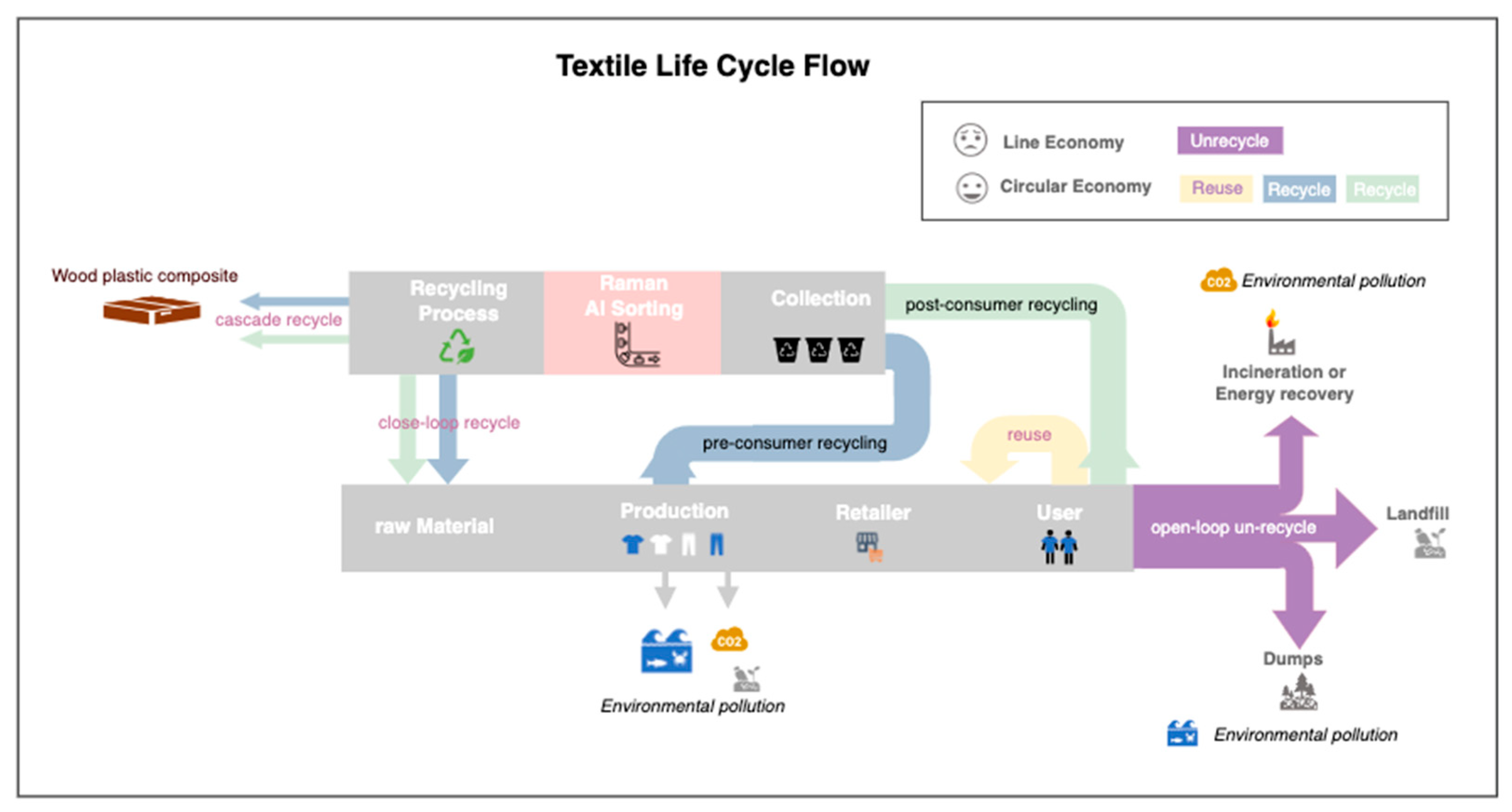
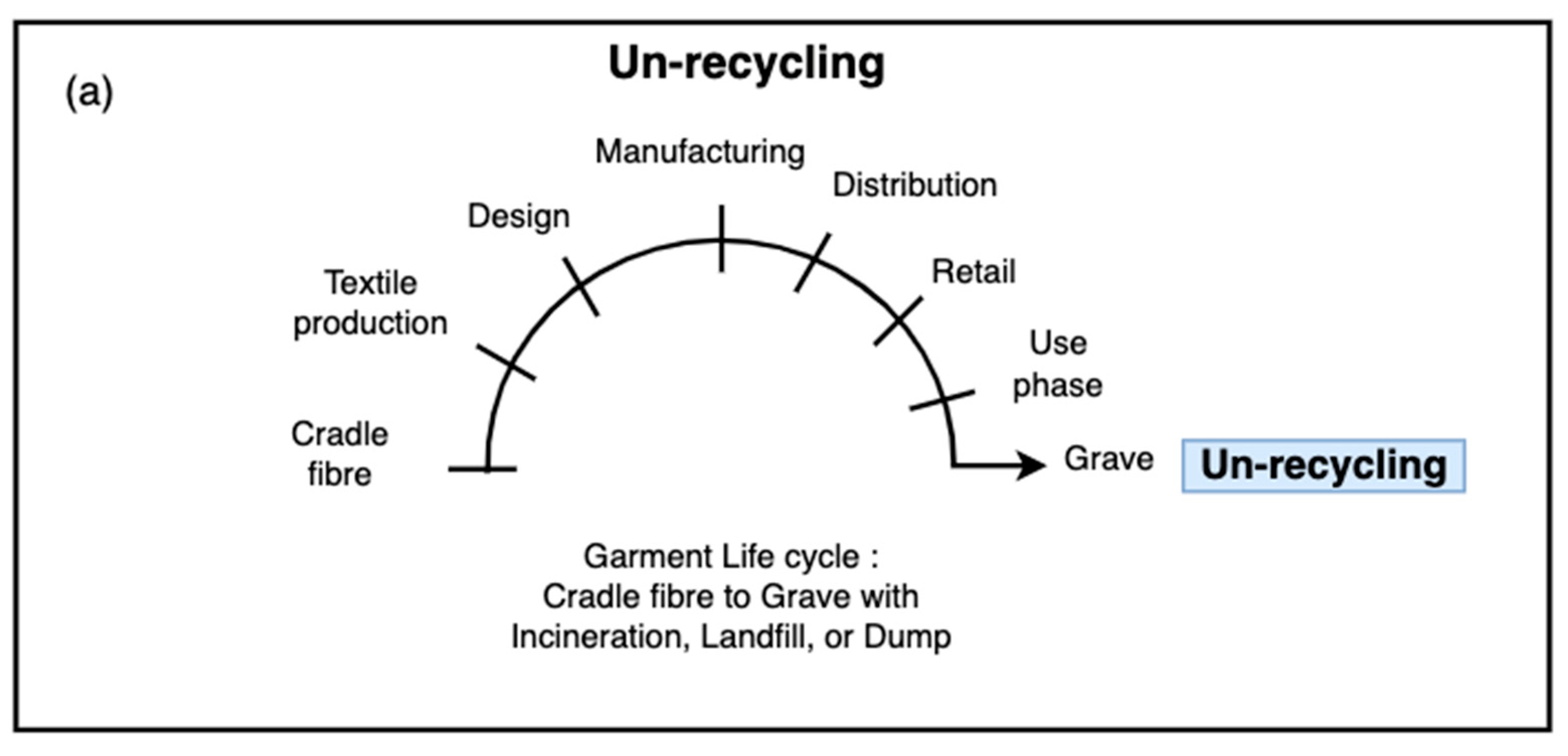
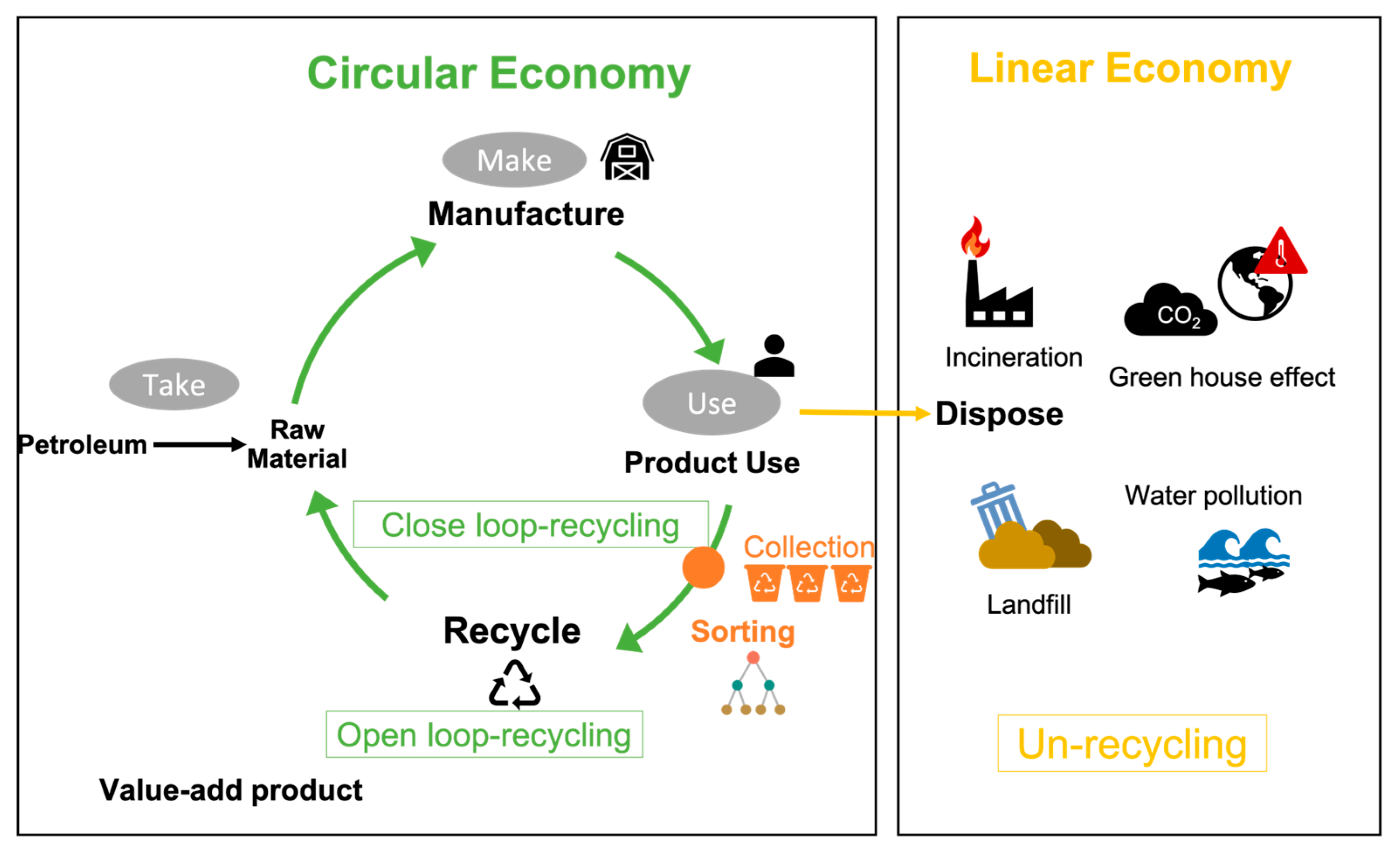
1.1. Textile Recycling and the Circular Economy
1.2. Challenges in Achieving a Circular Economy in the Textile Industry
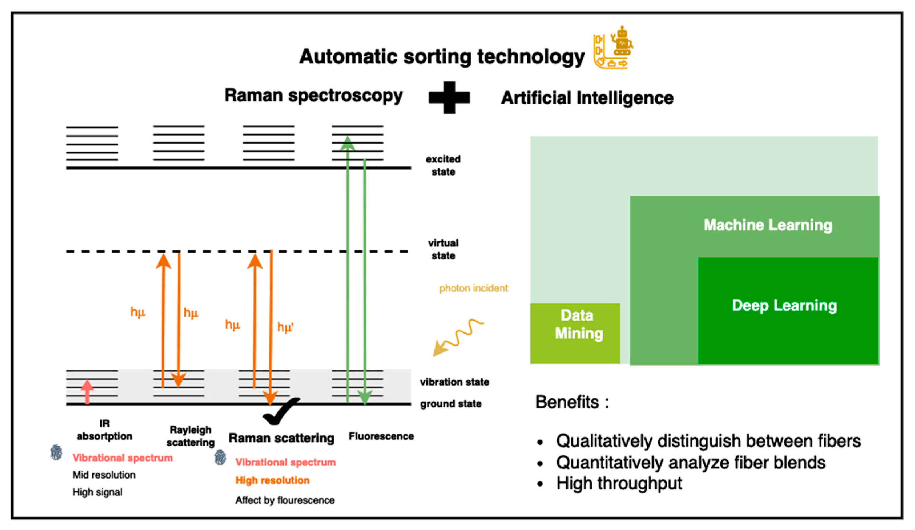
1.3. Vibrational Spectroscopy and AI for Textile Sorting
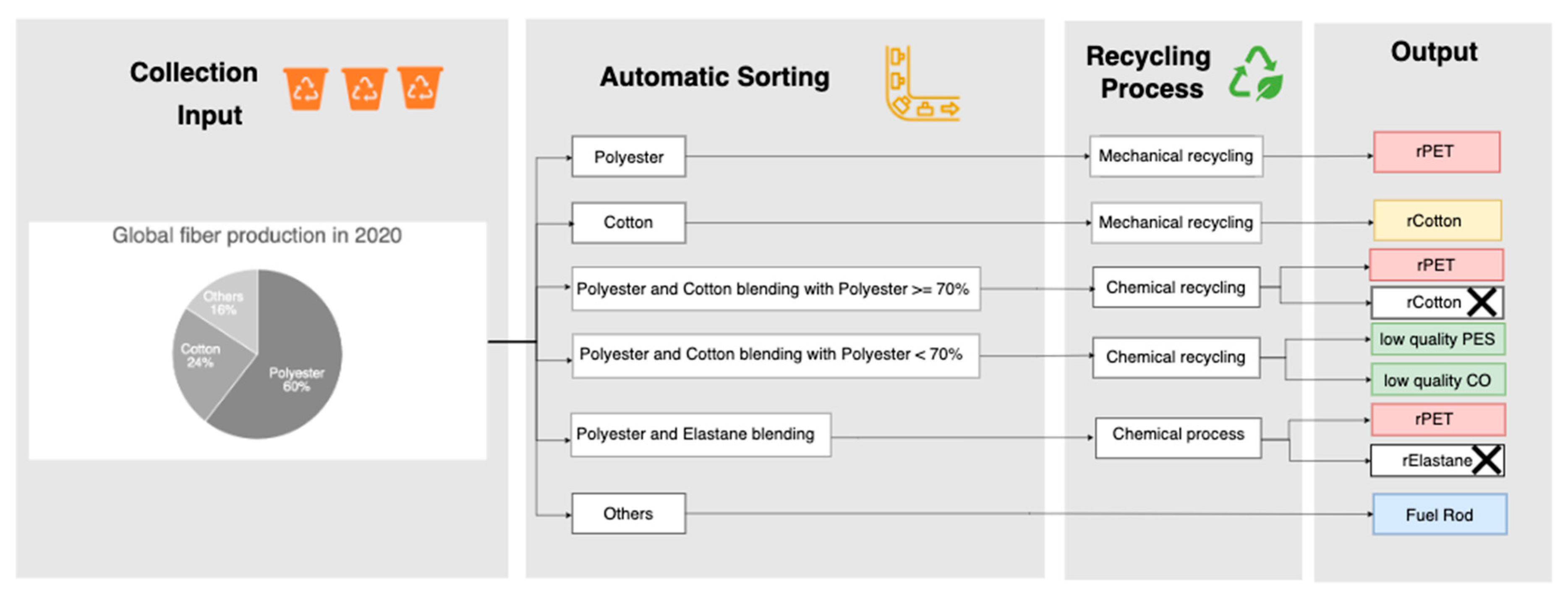
1.4. Importance of Sorting for rPET Recycling
1.5. Sorting and Recycling Processes for Different Textile Classes
1.5.1. 100% Cotton (CO)
- Reason for Sorting: Cotton is a natural fiber that can be efficiently recycled when not contaminated by synthetic materials. Sorting cotton ensures higher purity during recycling, leading to better-quality recycled cotton yarns or fibers;
- Recycling Method: Mechanical Recycling;
- Process: Cotton is shredded, cleaned, carded, and spun into new yarns for reuse;
- Recycling Outcome: High-quality recycled cotton yarns for new textile production.
1.5.2. 100% Polyester (PES)
- Reason for Sorting: Pure polyester can be recycled more efficiently compared to blends. The absence of cotton or other materials ensures that the recycling process can focus on re-polymerizing the polyester into rPET, maintaining its properties for reuse in high-quality textile products;
- Recycling Method: Mechanical Recycling;
- Process: Polyester textiles are shredded, cleaned, carded, and spun into yarns for reuse;
- Recycling Outcome: High-quality recycled polyester (rPET).
1.5.3. Polyester–Cotton Blends (PES/CO ≥ 70%)
- Reason for Sorting: Polyester–cotton blends with a higher percentage of polyester (≥70%) are common in the market because of their cost effectiveness and durability. Sorting these textiles allows for the efficient separation of polyester and cotton for recycling, enabling a higher yield of recycled polyester for rPET production;
- Recycling Method: Chemical Recycling;
- Separation Methods:
- Polyester Dissolution: Chemicals like DMSO dissolve polyester, leaving cotton intact. The polyester is recovered, purified, and re-polymerized into rPET;
- Cellulose Degradation: Cotton is broken down using hydrolysis, leaving behind pure polyester for rPET production;
- Recycling Outcome: High-quality rPET and cellulose for reuse.
1.5.4. Polyester–Cotton Blends (PES/CO < 70%)
- Reason for Sorting: Blends with less than 70% polyester are more challenging to recycle because of the increased presence of cotton. Sorting them separately ensures that a more appropriate recycling method is applied to maximize material recovery. This group often requires additional chemical or combined methods to effectively separate the fibers;
- Recycling Method: Mechanical or Combined Recycling;
- Process: Textiles are shredded and treated with chemical processes to separate polyester and cotton fibers;
- Recycling Outcome: Lower-quality recycled materials, potentially requiring virgin fibers to enhance product performance.
1.5.5. Polyester with Elastane (PES/EA)
- Reason for Sorting: Elastane is typically added in small quantities (<5%) to enhance the elastic properties of textiles, improving stretchability and comfort. Sorting these textiles ensures that the elastane content is taken into account when applying recycling methods, thereby preventing the contamination of recycled polyester and maintaining the quality of the final product;
- Recycling Method: Solvent-Based Recycling or Mechanical Shredding;
- Process:
- ○
- Solvent-Based Techniques: Selective solvents dissolve polyester while isolating elastane for further treatment;
- ○
- Mechanical Shredding: Elastane-contaminated polyester can be shredded into fibers, but this reduces the quality of recycled materials;
- Recycling Outcome: Recycled polyester with minimal elastane contamination, ensuring better-quality rPET.
1.5.6. Others: Blends with Polyamide (PA) or Other Fibers (Three or More Materials)
- Reason for Sorting: Textiles containing polyamide (PA), nylon, or three or more materials (such as polyester mixed with elastane, cotton, and polyamide) are highly complex and difficult to recycle. Sorting these textiles allows for the identification of the most appropriate recycling method for each fiber type, whether it involves downcycling or valorization to value-added products;
- Recycling Method: Downcycling or Valorization;
- Process: Textiles that cannot be efficiently separated are often downcycled to lower-quality products, like wood–plastic composites and insulation materials, or used for energy recovery;
- Recycling Outcome: Limited reuse and potential disposal if not sorted correctly.
1.6. Valorization and the Circular Economy
1.7. Enhancing the Circular Economy and Sustainability
- Utilizing automatic sorting technology—by integrating Raman spectroscopy with AI techniques, such as data mining, machine learning, and deep learning—we can enhance the circular economy and sustainability, as shown in Figure 8, as follows:
- ○
- Enhance closed-loop recycling efficiency with high-purity PET textiles;
- ○
- Divert low-purity textiles to open-loop recycling, ensuring alternative uses instead of disposal;
- ○
- Support waste textile valorization, turning waste into value-added products that contribute to resource sustainability;
- ○
- This approach transforms the textile life cycle from an un-recycling linear economy to a circular economy, minimizing waste, reducing environmental pollution, and ensuring sustainable textile management.
2. Literature Review
2.1. Raman Spectroscopy in Fiber and Textile Analysis
2.2. Machine-Learning and Deep-Learning Models for Raman Spectroscopy
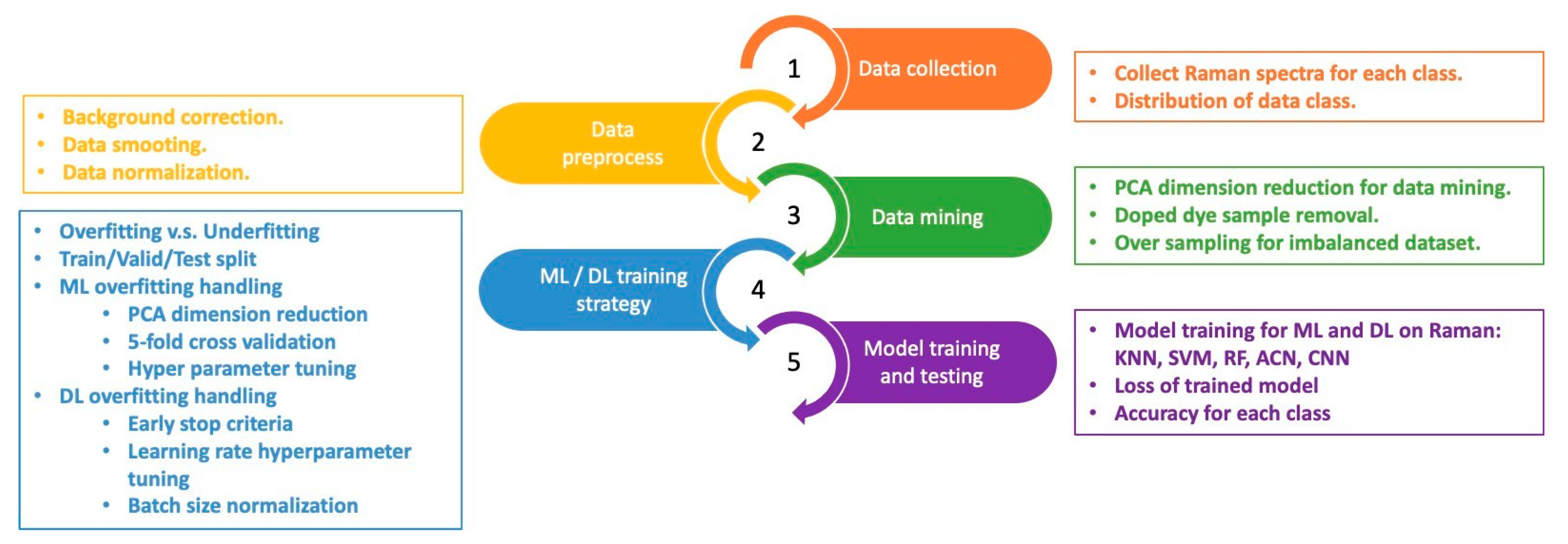
3. Methodology
3.1. Textile Labeling with FTIR Spectroscopy
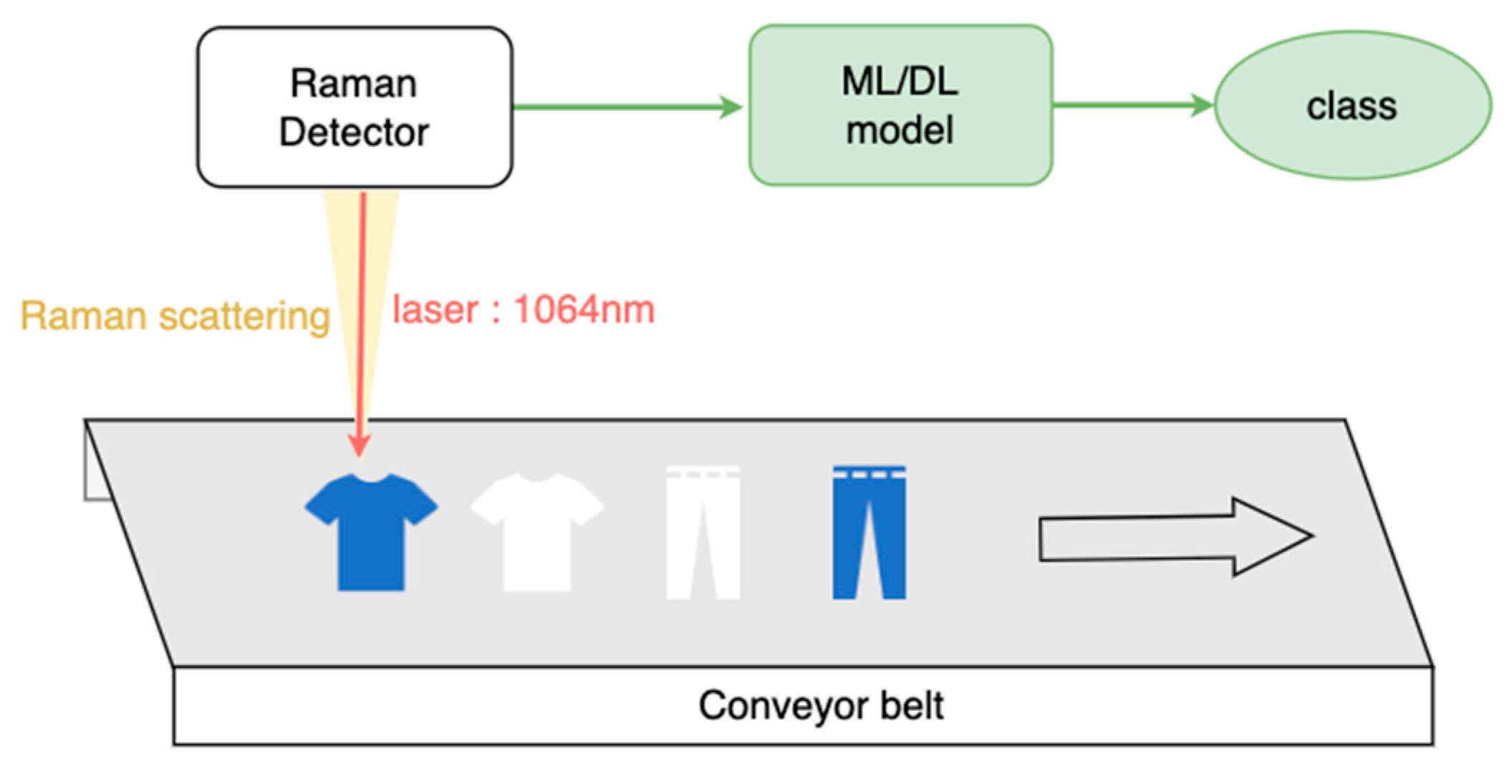
3.2. Raman Online Hardware
- Conveyer speed: 40 cm/s;
- Camera integration time: 1 s;
- Excitation laser wavelength: 1064 nm;
- Raman spectral range: −1775~3597 cm−1;
- Sampling Z-height scan for signal optimization;
- Detection speed: 1 s per piece.
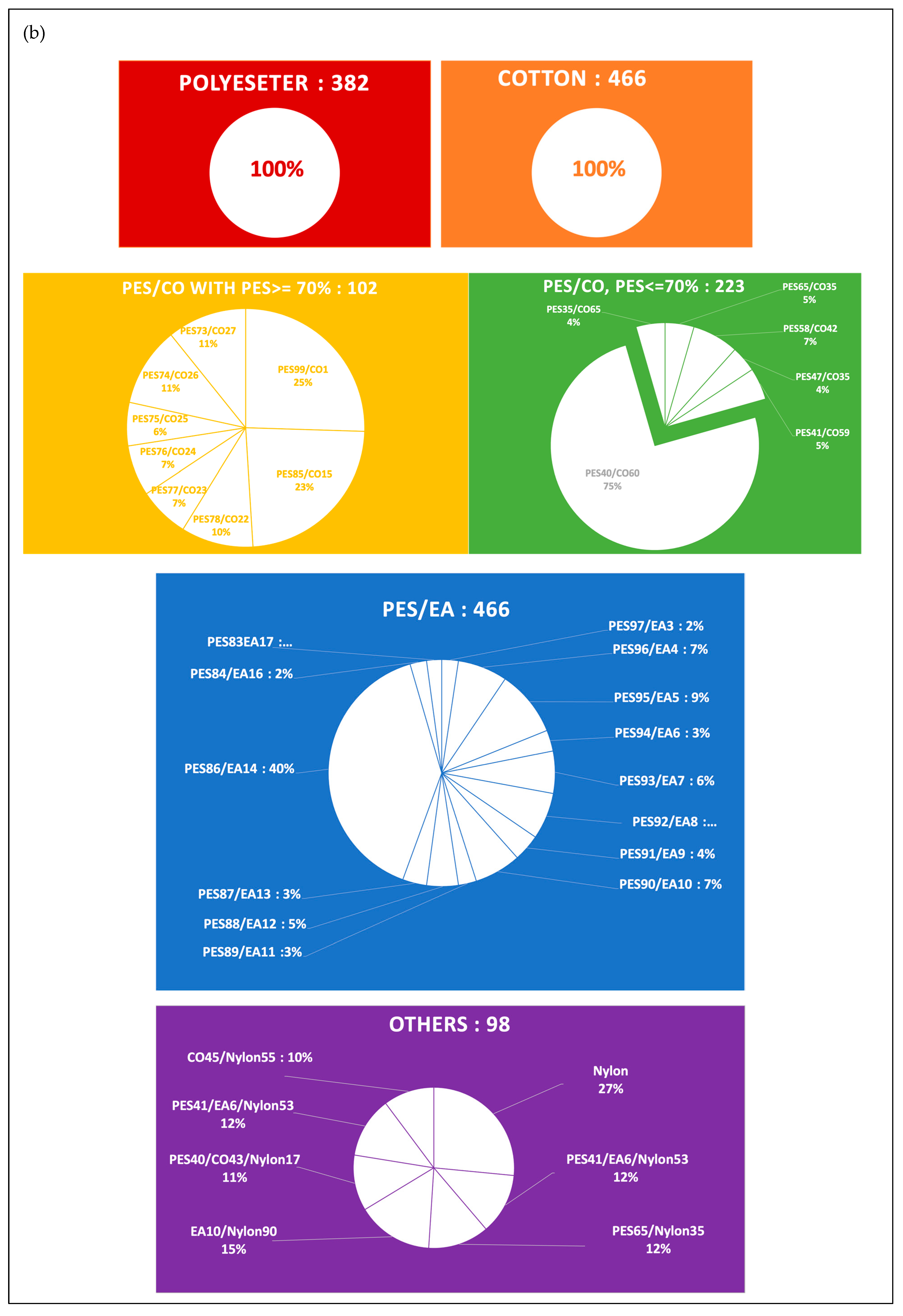
3.3. Data Collection and Label Distribution
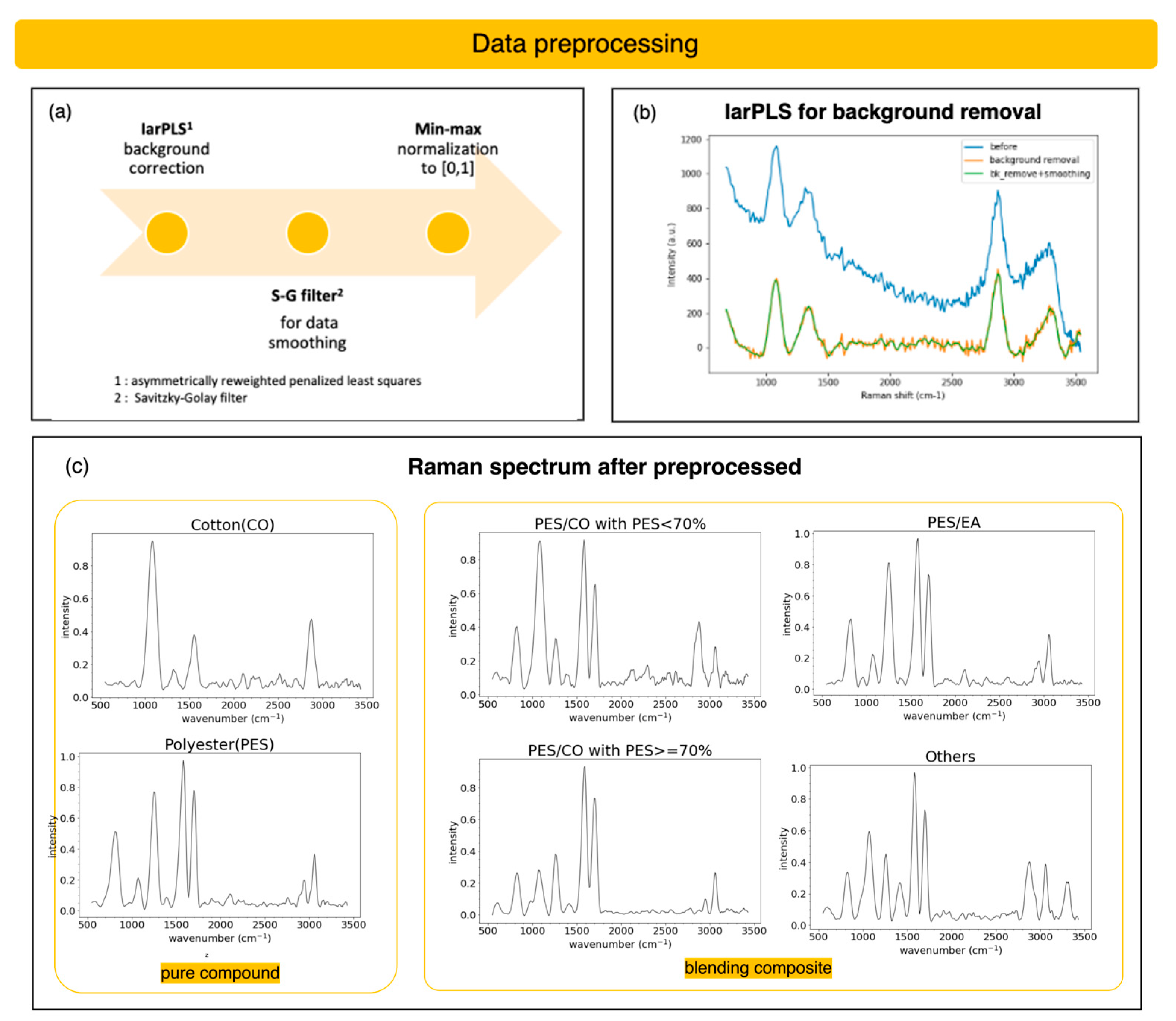
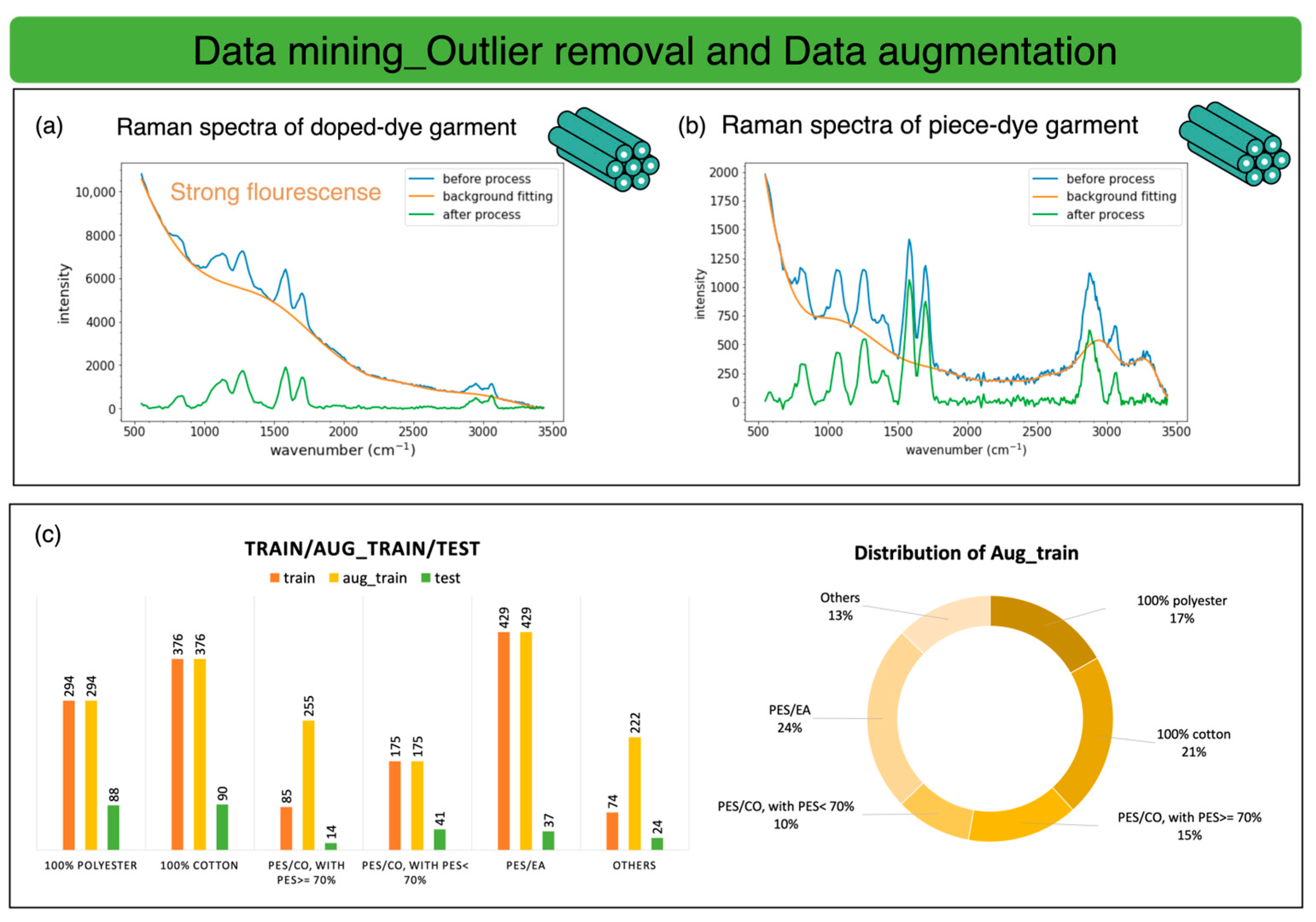
3.4. Data Preprocessing for Fluorescence Background Reduction and Outlier Removal
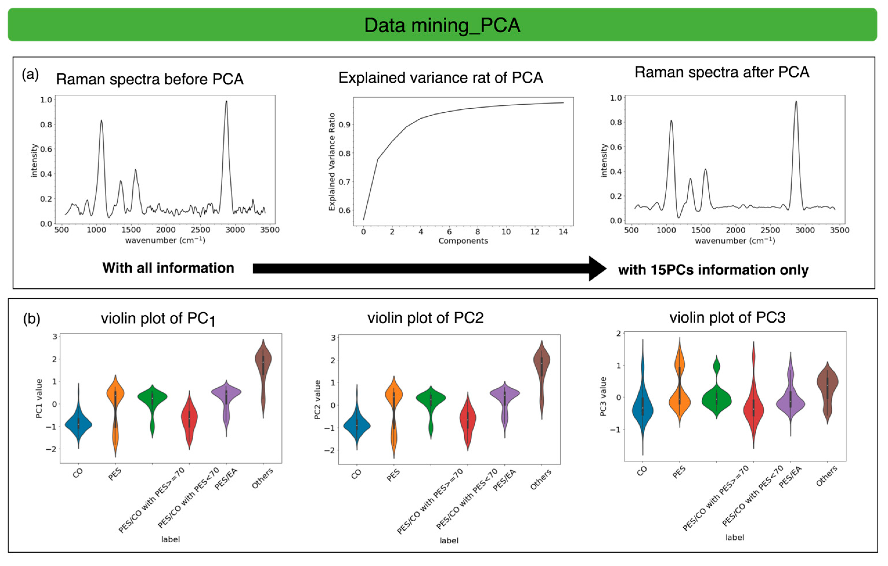
3.5. Data Mining with PCA and Outlier Removal
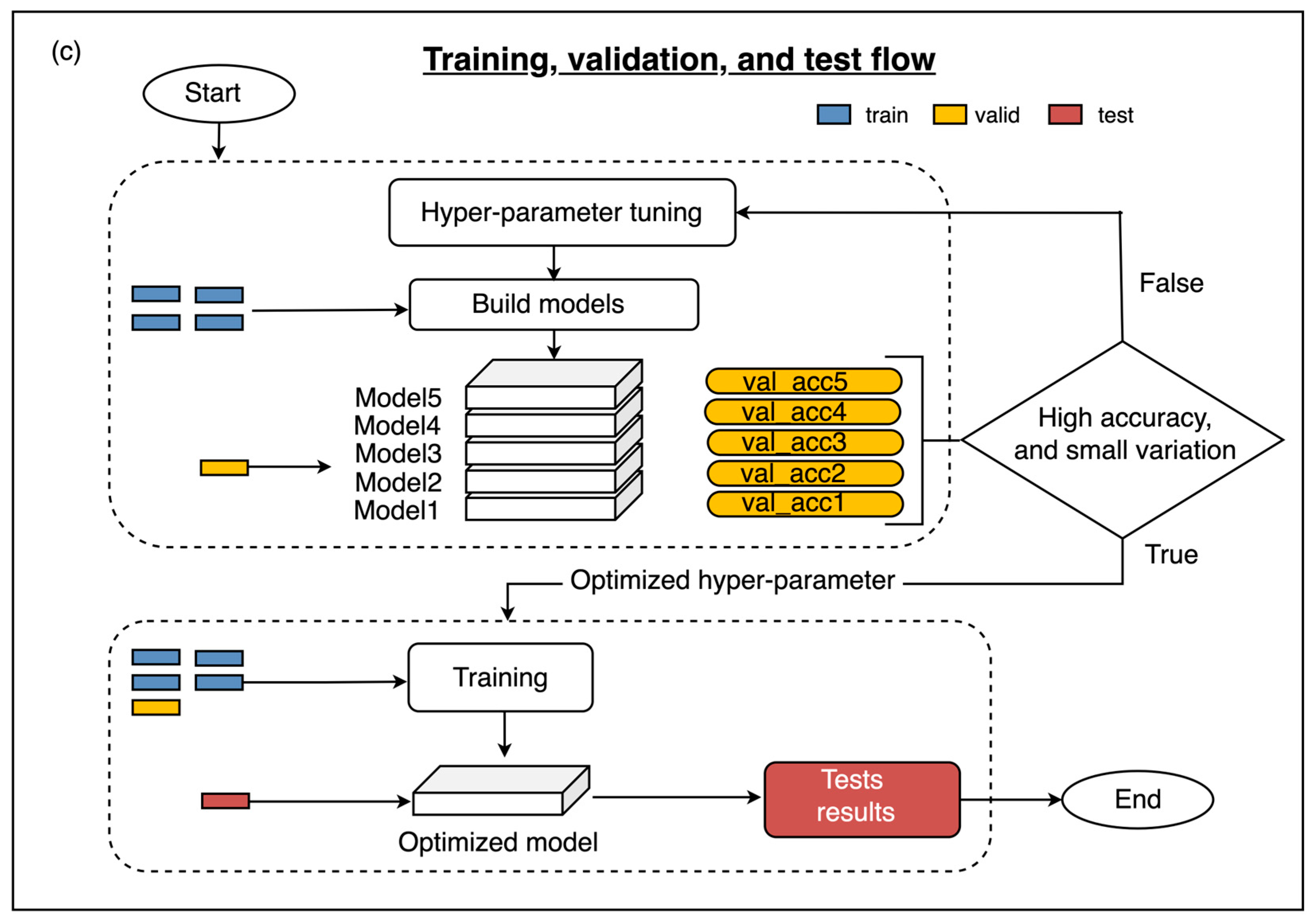
3.6. Model-Training Strategy
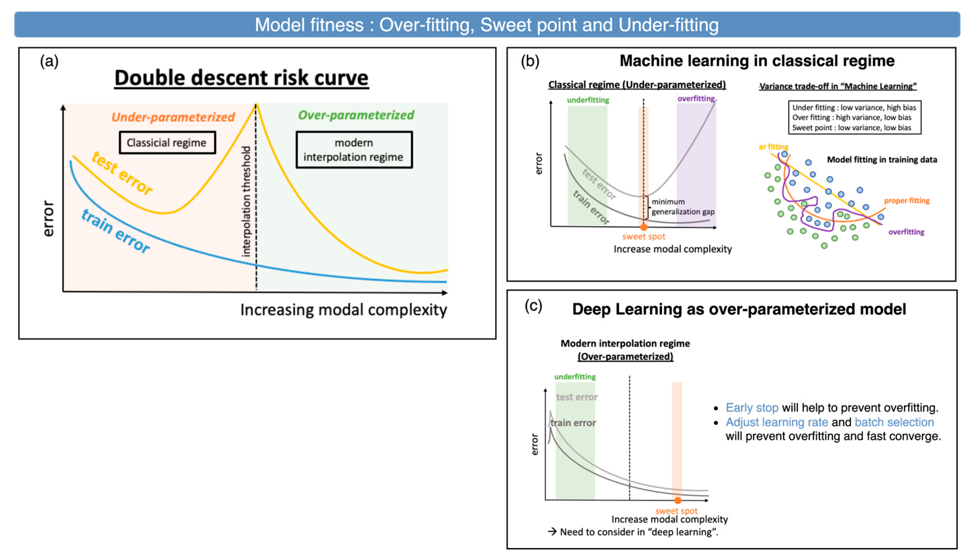
3.6.1. Model Fitness
3.6.2. Machine-Learning Optimization Strategy
3.6.3. Deep-Learning Optimization Strategy
3.7. Model-Training and -Testing Accuracy
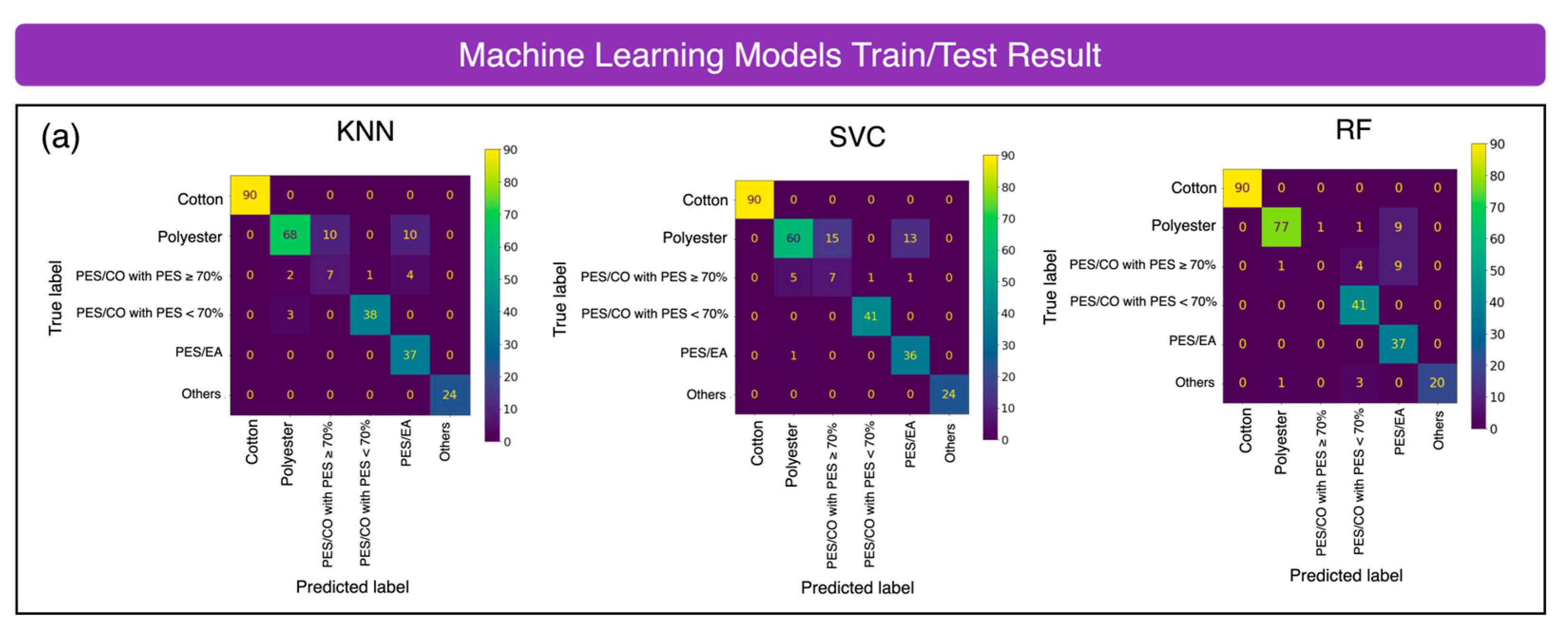
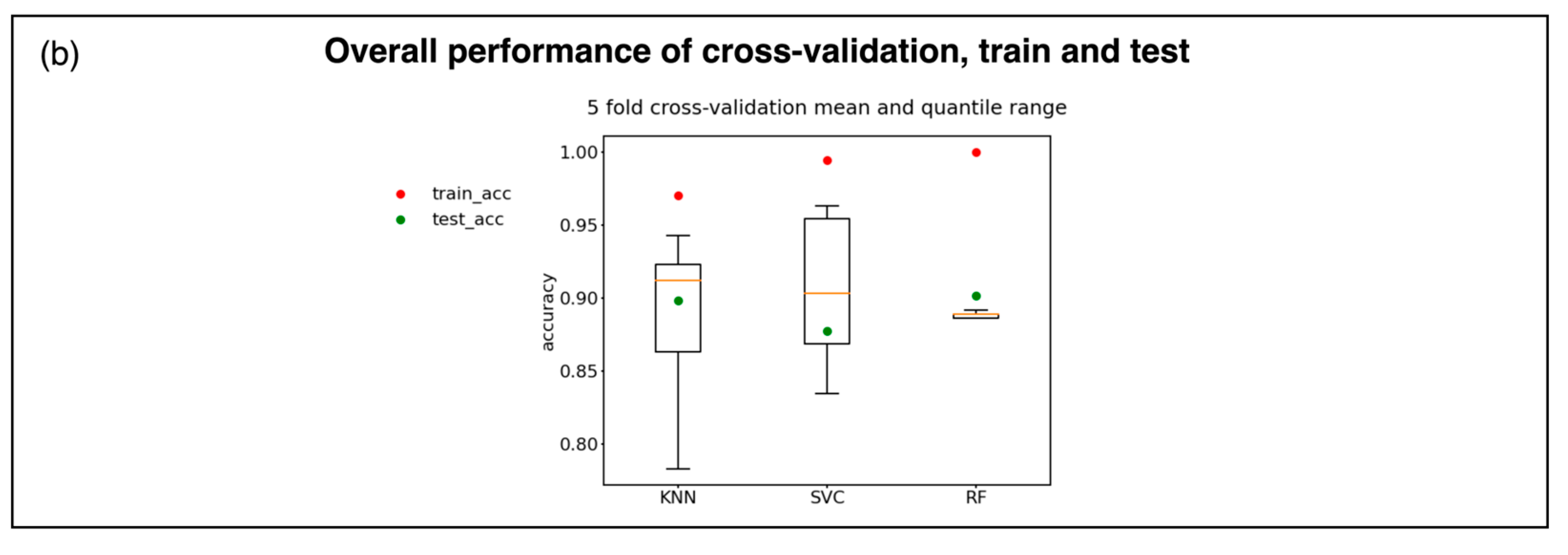
3.7.1. Machine-Learning Training and Testing Accuracies
- K-Nearest Neighbors (KNNs) [24]
- Random Forest (RF) [26]
- Machine learning performance comparison:
3.7.2. Deep-Learning Training and Testing Accuracies
- Artificial Neural Network (ANN)
- Learning rate: 0.001;
- Number of learning epochs: 200;
- Batch size: 128;
- Optimizer: Adam [58];
- Convolutional neural network (CNN).
- Learning rate: 0.001;
- Number of learning epochs: 200;
- Batch size: 128;
- Optimizer: Adam [58].
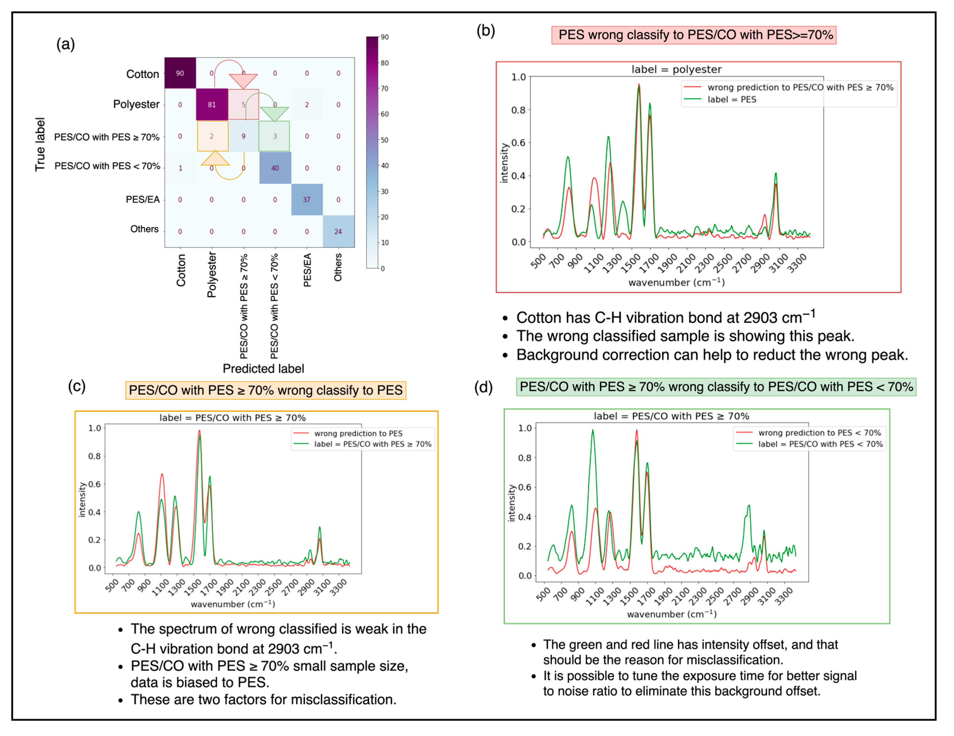
3.8. Misclassification Check for the ANN Model
4. Results and Discussion
5. Conclusions
5.1. Raman Spectroscopy with AI for Waste Textile Sorting
- High Degree of Accuracy in Fiber Type Classification: Achieving over 95% accuracy in distinguishing between fiber types;
- High Degree of Accuracy in Blend Compositional Analysis: Achieving over 95% accuracy in analyzing blended-fiber compositions;
- High Throughput: Enabling automatic sorting at a speed of one piece per second, replacing manual sorting processes.
5.2. Data Preprocessing for Enhanced AI Modeling
- Dimensionality Reduction: Enhancing machine-learning models by reducing complexity;
- Balanced Dataset Preparation: Ensuring clean and relatively balanced datasets for effective model training;
- Fluorescence Signal Reduction: Removing dyes’ fluorescence signals to retain only vibrational spectral information essential for AI modeling.
5.3. Achieving Qualitative and Quantitative Sorting with High Degrees of Accuracy and Efficiency
- Closed-Loop Recycling: Sorting purer textiles for recycling into high-quality recycled PES fibers;
- Open-Loop Recycling: Valorizing waste textiles to value-added products, such as wood–plastic composites [14];
- By improving recycling rates and extending textile lifespans, this technology helps to meet the demand for recycled polyester and supports a circular economy.
5.4. Future Directions
- Expanding Textiles’ Raman Spectral Datasets: Reducing data imbalance, particularly for textile classes like PES/CO with PES ≥ 70%, through dataset expansion;
- Integrated Background Correction: Utilizing autoencoders, for self-adaptive learning to correct for background interference, seamlessly connected to ANN or CNN networks for one-stage classification.
Author Contributions
Funding
Institutional Review Board Statement
Informed Consent Statement
Data Availability Statement
Conflicts of Interest
Abbreviations
| Abbreviation | Definition |
| 3R | reduction, reuse, and recycling |
| AI | artificial intelligence |
| ANN | artificial neural network |
| CE | circular economy |
| CLR | closed-loop recycling |
| CNN | convolutional neural network |
| CO | cotton |
| DL | deep learning |
| EA | elastance (spandex) |
| ESG | environmentally sustainable governance |
| FTIR | Fourier-transform infrared |
| IRS | infrared spectroscopy |
| ITRI | Industrial Technology Research Institute |
| kNN | k-nearest neighbor |
| LCA | life cycle assessment |
| ML | machine learning |
| NIRS | near-infrared spectroscopy |
| OLR | open-loop recycling |
| PC | principal component |
| PCA | principal component analysis |
| PES | polyester |
| PES/CO | polyester and cotton blend |
| PES/EA | polyester and elastance blend |
| PA | polyamide |
| RF | random forest |
| rPET | recycled polyethylene terephthalate |
| S-G filter. | Savitzky–Golay filter |
| SVM | support vector machine |
References
- Stegmann, P.; Daioglou, V.; Londo, M.; Vuuren, D.P.V.; Junginger, M. Plastic futures and their CO2 emissions. Nature 2022, 612, 272–276. [Google Scholar] [CrossRef]
- Geyer, R.; Jambeck, J.R.; Law, K.L. Production, use, and fate of all plastics ever made. Sci. Adv. 2017, 3, e1700782. [Google Scholar] [CrossRef] [PubMed]
- MDBC. A New Life for Fabrics and Plastics; Malaysia Dutch Business Council: Kuala Lumpur, Malaysia, 2021; Available online: https://www.mdbc.com.my/wp-content/uploads/2021/12/M4M-Environmental-Business-Kloth.pdf (accessed on 19 December 2024).
- Payne, A. Open-and closed-loop recycling of textile and apparel products. In Handbook of Life Cycle Assessment (LCA) of Textiles and Clothing; Woodhead Publishing Series in Textiles: Delhi, India, 2015; pp. 103–123. [Google Scholar] [CrossRef]
- Rudisch, K.; Jüngling, S.; Mendoza, R.C.; Woggon, U.K.; Budde, I.; Malzacher, M.; Pufahl, K. Paving the road to a circular textile economy with AI. In Informatik 2021; Gesellschaft für Informatik: Bonn, Germany, 2021; pp. 313–320. [Google Scholar] [CrossRef]
- Sathyanarayana, D.N. Vibrational Spectroscopy: Theory and Applications; New Age International Publisher: Delhi, India, 2015. [Google Scholar]
- Pasquini, C. Near infrared spectroscopy: A mature analytical technique with new perspectives—A review. Anal. Chim. Acta 2018, 1026, 8–36. [Google Scholar] [CrossRef]
- Long, D.A. The Characterization of Chemical Purity Organic Compounds; Staveley, L.A.K., Ed.; Elviser: Amsterdam, The Netherlands, 1977; pp. 149–162. [Google Scholar]
- Lyon, L.A.; Keating, C.D.; Fox, A.P.; Baker, B.E.; He, L.; Nicewarner, S.R.; Mulvaney, S.P.; Natan, M.J. Raman spectroscopy. Anal. Chem. 1998, 70, 341–362. [Google Scholar] [CrossRef] [PubMed]
- Mulvaney, S.P.; Keating, C.D. Raman spectroscopy. Anal. Chem. 2000, 72, 145–158. [Google Scholar] [CrossRef]
- Muthu, S.S.; Li, Y.; Hu, J.Y.; Mok, P.Y. Recyclability Potential Index (RPI): The concept and quantification of RPI for textile fibres. Ecol. Indic. 2012, 18, 58–62. [Google Scholar] [CrossRef]
- Ling, C.; Shi, S.; Hou, W.; Yan, Z. Separation of waste polyester/cotton blended fabrics by phosphotungstic acid and preparation of terephthalic acid. Polym. Degrad. Stab. 2019, 161, 157–165. [Google Scholar] [CrossRef]
- Wang, H.; Kaur, G.; Pensupa, N.; Uisan, K.; Du, C.; Yang, X.; Lin, C.S.K. Textile waste valorization using submerged filamentous fungal fermentation. Process Saf. Environ. Prot. 2018, 118, 143–151. [Google Scholar] [CrossRef]
- Subramanian, K.; Sarkar, M.K.; Wang, H.; Qin, Z.H.; Chopra, S.S.; Jin, M.; Kumar, V.; Chen, C.; Tsang, C.W.; Lin, C.S.K. An overview of cotton and polyester, and their blended waste textile valorisation to value-added products: A circular economy approach–research trends, opportunities and challenges. Crit. Rev. Environ. Sci. Technol. 2022, 52, 3921–3942. [Google Scholar] [CrossRef]
- Hou, W.; Ling, C.; Shi, S.; Yan, Z.; Zhang, M.; Zhang, B.; Dai, J. Separation and characterization of waste cotton/polyester blend fabric with hydrothermal method. Fibers Polym. 2018, 19, 742–750. [Google Scholar] [CrossRef]
- Islam, S.; Ahmed, S.; Arifuzzaman, M.; Islam, A.S.; Akter, S. Relationship in between strength and polyester content percentage of cotton polyester blended woven fabrics. Int. J. Cloth. Sci. 2019, 6, 1–6. [Google Scholar]
- Kudelski, A. Analytical applications of Raman spectroscopy. Talanta 2008, 76, 1–8. [Google Scholar] [CrossRef] [PubMed]
- Wiley, J.H.; Atalla, R.H. Band assignments in the Raman spectra of celluloses. Carbohydr. Res. 1987, 160, 113–129. [Google Scholar] [CrossRef]
- Edwards, H.; Farwell, D.; Webster, D. FT Raman microscopy of untreated natural plant fibres. Spectrochim. Acta Part A Mol. Biomol. Spectrosc. 1997, 53, 2383–2392. [Google Scholar] [CrossRef]
- Kavkler, K.; Demšar, A. Examination of cellulose textile fibres in historical objects by micro-Raman spectroscopy. Spectrochim. Acta Part A Mol. Biomol. Spectrosc. 2011, 78, 740–746. [Google Scholar] [CrossRef]
- Carey, C.; Boucher, T.; Mahadevan, S.; Bartholomew, P.; Dyar, M. Machine learning tools formineral recognition and classification from Raman spectroscopy. J. Raman Spectrosc. 2015, 46, 894–903. [Google Scholar] [CrossRef]
- Guo, S.; Popp, J.; Bocklitz, T. Chemometric analysis in Raman spectroscopy from experimental design to machine learning-based modeling. Nat. Protoc. 2021, 16, 5426–5459. [Google Scholar] [CrossRef]
- Qi, Y. Recent progresses in machine learning assisted Raman spectroscopy. Adv. Opt. Mater. 2023, 11, 2203104. [Google Scholar] [CrossRef]
- Peterson, L.E. K-nearest neighbor. Scholarpedia 2009, 4, 1883. [Google Scholar] [CrossRef]
- Myles, A.J.; Feudale, R.N.; Liu, Y.; Woody, N.A.; Brown, S.D. An introduction to decision tree modeling. J. Chemom. 2004, 18, 275–285. [Google Scholar] [CrossRef]
- Biau, G.; Scornet, E. A random forest guided tour. Test 2016, 25, 197–227. [Google Scholar] [CrossRef]
- Burges, C.J. A tutorial on support vector machines for pattern recognition. Data Min. Knowl. Discov. 1998, 2, 121–167. [Google Scholar] [CrossRef]
- Gunn, S.R. Support vector machines for classification and regression. ISIS Tech. Rep. 1998, 14, 5–16. [Google Scholar]
- Furey, T.S.; Cristianini, N.; Duffy, N.; Bednarski, D.W.; Schummer, M.; Haussler, D. Support vector machine classification and validation of cancer tissue samples using microarray expression data. Bioinformatics 2000, 16, 906–914. [Google Scholar] [CrossRef]
- Finkelstein, M.O.; Fairley, W.B. A Bayesian approach to identification evidence. Harv. Law Rev. 1970, 83, 489–517. [Google Scholar] [CrossRef]
- Yegnanarayana, B. Artificial Neural Networks; PHI Learning Pvt. Ltd.: Delhi, India, 2009. [Google Scholar]
- Albawi, S.; Mohammed, T.A.; Al-Zawi, S. Understanding of a convolutional neural network. In Proceedings of the 2017 International Conference on Engineering and Technology (ICET), Antalya, Turkey, 21–23 August 2017; Volume 10. [Google Scholar]
- Schuster, M.; Paliwal, K.K. Bidirectional recurrent neural networks. IEEE Trans. Signal Process. 1997, 45, 2673–2681. [Google Scholar] [CrossRef]
- Goodfellow, I.; Pouget-Abadie, J.; Mirza, M.; Xu, B.; Warde-Farley, D.; Ozair, S.; Courville, A.; Bengio, Y. Generative adversarial nets. Adv. Neural Inf. Process. System 2014, 27, 1–9. Available online: https://proceedings.neurips.cc/paper_files/paper/2014/file/5ca3e9b122f61f8f06494c97b1afccf3-Paper.pdf (accessed on 19 December 2024).
- Fan, X.; Ming, W.; Zeng, H.; Zhang, Z.; Lu, H. Deep learning-based component identification for the Raman spectra of mixtures. Analyst 2019, 144, 1789–1798. [Google Scholar] [CrossRef]
- Ho, C.S. Rapid identification of pathogenic bacteria using Raman spectroscopy and deep learning. Nat. Commun. 2019, 10, 4927. [Google Scholar] [CrossRef]
- Ralbovsky, N.M.; Lednev, I.K. Towards development of a novel universal medical diagnostic method: Raman spectroscopy and machine learning. Chem. Soc. Rev. 2020, 49, 7428–7453. [Google Scholar] [CrossRef] [PubMed]
- Neo, E.R.K.; Yeo, Z.; Low, J.S.C.; Goodship, V.; Debattista, K. A review on chemometric techniques with infrared, Raman and laser-induced breakdown spectroscopy for sorting plastic waste in the recycling industry. Resour. Conserv. Recycl. 2022, 180, 106217. [Google Scholar] [CrossRef]
- Maruthamuthu, M.K.; Raffiee, A.H.; Oliveira, D.M.D.; Ardekani, A.M.; Verma, M.S. Raman spectra-based deep learning: A tool to identify microbial contamination. MicrobiologyOpen 2020, 9, e1122. [Google Scholar] [CrossRef] [PubMed]
- Kow, P.Y.; Hsia, I.W.; Chang, L.C.; Chang, F.J. Real-time image-based air quality estimation by deep learning neural networks. J. Environ. Manag. 2022, 307, 114560. [Google Scholar] [CrossRef]
- Industrial Technology Research Institute. Available online: https://www.itri.org.tw/english/index.aspx (accessed on 19 December 2024).
- Online Raman Textile Sorter in ITRI. Available online: https://www.itri.org.tw/ListStyle.aspx?DisplayStyle=01_content&SiteID=1&MmmID=1036233376244004650&MGID=1163436641542114306 (accessed on 19 December 2024).
- Castro, M.; Pereira, F.; Aller, A.; Littlejohn, D. Raman spectrometry as a screening tool for solvent-extracted azo dyes from polyester-based textile fibres. Polym. Test. 2020, 91, 106765. [Google Scholar] [CrossRef]
- Ye, J.; Tian, Z.; Wei, H.; Li, Y. Baseline correction method based on improved asymmetrically reweighted penalized least squares for the Raman spectrum. Appl. Opt. 2020, 59, 10933–10943. [Google Scholar] [CrossRef] [PubMed]
- Savitzky, A.; Golay, M.J. Smoothing and differentiation of data by simplified least squares procedures. Anal. Chem. 1964, 36, 1627–1639. [Google Scholar] [CrossRef]
- Schafer, R.W. What is a Savitzky-Golay filter? IEEE Signal Process. Mag. 2011, 28, 111–117. [Google Scholar] [CrossRef]
- Belkin, M.; Hsu, D.; Ma, S.; Mandal, S. Reconciling modern machine-learning practice and the classical bias-variance trade-off. Proc. Natl. Acad. Sci. USA 2019, 116, 15849–15854. [Google Scholar] [CrossRef] [PubMed]
- Mathew, A.; Amudha, P.; Sivakumari, S. Deep learning techniques: An overview. In Advanced Machine Learning Technologies and Applications: Proceedings of AMLTA 2020; Springer: Singapore, 2021; pp. 599–608. [Google Scholar]
- Li, S.; Song, W.; Fang, L.; Chen, Y.; Ghamisi, P.; Benediktsson, J.A. Deep learning for hyperspectral image classification: An overview. IEEE Trans. Geosci. Remote Sens. 2019, 57, 6690–6709. [Google Scholar] [CrossRef]
- Cheng, H.T.; Koc, L.; Harmsen, J.; Shaked, T.; Chandra, T.; Aradhye, H.; Anderson, G.; Corrado, G.; Chai, W.; Ispir, M.; et al. Wide & deep learning for recommender systems. In Proceedings of the 1st Workshop on Deep Learning for Recommender Systems, New York, NY, USA, 15 September 2016; pp. 7–10. [Google Scholar]
- Zhao, Z.Q.; Zheng, P.; Xu, S.T.; Wu, X. Object detection with deep learning: A review. IEEE Trans. Neural Netw. Learn. Syst. 2019, 30, 3212–3232. [Google Scholar] [CrossRef]
- Prechelt, L. Automatic early stopping using cross validation: Quantifying the criteria. Neural Netw. 1998, 11, 761–767. [Google Scholar] [CrossRef] [PubMed]
- Gotmare, A.; Keskar, N.S.; Xiong, C.; Socher, R. A closer look at deep learning heuristics: Learning rate restarts, warmup and distillation. arXiv 2018, arXiv:1810.13243. [Google Scholar] [CrossRef]
- Smith, S.L.; Kindermans, P.J.; Ying, C.; Le, Q.V. Don’t decay the learning rate, increase the batch size. arXiv 2017, arXiv:1711.00489. [Google Scholar] [CrossRef]
- Scholkopf, B.; Sung, K.K.; Burges, C.J.; Girosi, F.; Niyogi, P.; Poggio, T.; Vapnik, V. Comparing support vector machines with Gaussian kernels to radial basis function classifiers. IEEE Trans. Signal Process. 1997, 45, 2758–2765. [Google Scholar] [CrossRef]
- Luo, R.; Popp, J.; Bocklitz, T. Deep learning for Raman spectroscopy: A review. Analytica 2022, 3, 287–301. [Google Scholar] [CrossRef]
- Misra, D. Mish: A self regularized non-monotonic activation function. arXiv 2019, arXiv:1908.08681. [Google Scholar] [CrossRef]
- Kingma, D.P.; Ba, J. Adam: A method for stochastic optimization. arXiv 2014, arXiv:1412.6980. [Google Scholar] [CrossRef]
- Krizhevsky, A.; Hinton, G. Convolutional deep belief networks on cifar 10. Unpubl. Manuscr. 2010, 40, 1–9. [Google Scholar]
- Deng, J.; Dong, W.; Socher, R.; Li, L.J.; Li, K.; Fei-Fei, L. Imagenet: A large-scale hierarchical image database. In Proceedings of the IEEE Conference on Computer Vision and Pattern Recognition, Miami, FL, USA, 20–25 June 2009; pp. 248–255. [Google Scholar] [CrossRef]
- Ramachandran, P.; Zoph, B.; Le, Q.V. Swish: A self-gated activation function. arXiv 2017, arXiv:1710.05941. [Google Scholar] [CrossRef]
- Puchowicz, D.; Cieslak, M. Raman spectroscopy in the analysis of textile structures. In Recent Developments in Atomic Force Microscopy and Raman Spectroscopy for Materials Characterization; IntechOpen: London, UK, 2022; pp. 1–21. [Google Scholar] [CrossRef]
- Grady, A.; Dennis, A.C.; Denvir, D.; Mcgarvey, J.J.; Bell, S.E. Quantitative Raman spectroscopy of highly fluorescent samples using pseudosecond derivatives and multivariate analysis. Anal. Chem. 2001, 73, 2058–2065. [Google Scholar] [CrossRef] [PubMed]
- Chequer, F.D.; de Oliveira, G.A.R.; Ferraz, E.A.; Cardoso, J.C.; Zanoni, M.B.; de Oliveira, D.P. Textile dyes: Dyeing process and environmental impact. In Eco-Friendly Textile Dyeing and Finishing; IntechOpen Limited: London, UK, 2013; Volume 6, pp. 151–176. Available online: https://www.intechopen.com/chapters/41411 (accessed on 19 December 2024).
- Varadarajan, G.; Venkatachalam, P. Sustainable textile dyeing processes. Environ. Chem. Lett. 2016, 14, 113–122. [Google Scholar] [CrossRef]
- Yaseen, D.; Scholz, M. Textile dye wastewater characteristics and constituents of synthetic effluents: A critical review. Int. J. Environ. Sci. Technol. 2019, 16, 1193–1226. [Google Scholar] [CrossRef]
- Vaswani, A.; Shazeer, N.; Parmar, N.; Uszkoreit, J.; Jones, L.; Gomez, A.N.; Kaiser, Ł.; Polosukhin, I. Attention is all you need. In Proceedings of the Neural Information Processing Systems (NIPS 2017), Long Beach, CA, USA, 4–9 December 2017; Volume 30. Available online: https://proceedings.neurips.cc/paper_files/paper/2017/file/3f5ee243547dee91fbd053c1c4a845aa-Paper.pdf (accessed on 19 December 2024).
- Chang, M.; He, C.; Du, Y.; Qiu, Y.; Wang, L.; Chen, H. RaT: Raman Transformer for highly accurate melanoma detection with critical features visualization. Spectrochim. Acta Part A Mol. Biomol. Spectrosc. 2024, 305, 123475. [Google Scholar] [CrossRef]


| KNN | SVC | RF | ||
|---|---|---|---|---|
| Five fold cross-validation | Validation accuracy | 88.40% | 99.00% | 100.00% |
| Validation STD | 5.70% | 4.90% | 0.43% | |
| Training accuracy | 97.00% | 90.40% | 91.40% | |
| Testing accuracy | 89.50% | 88.00% | 90.00% | |
| KNN | SVC | RF | ANN | CNN | |
|---|---|---|---|---|---|
| Training accuracy | 97.00% | 90.40% | 91.40% | 96.20% | 98.00% |
| Validation accuracy | 88.40% | 99.00% | 100.00% | 93.50% | 97.00% |
| Testing accuracy | 89.50% | 88.00% | 90.00% | 96.90% | 93.50% |
| Fabric Type | Number of Samples | Number of Samples Correctly Classified | Accuracy of the ANN Model (%) |
|---|---|---|---|
| Cotton (CO) | 90 | 90 | 100.0% |
| Polyester (PES) | 88 | 81 | 92.0% |
| PES/CO with PES ≥ 70% | 14 | 9 | 64.3% |
| PES/CO with PES < 70% | 41 | 40 | 97.5% |
| PES/EA | 37 | 37 | 100.0% |
| Others | 24 | 24 | 100.0% |
Disclaimer/Publisher’s Note: The statements, opinions and data contained in all publications are solely those of the individual author(s) and contributor(s) and not of MDPI and/or the editor(s). MDPI and/or the editor(s) disclaim responsibility for any injury to people or property resulting from any ideas, methods, instructions or products referred to in the content. |
© 2024 by the authors. Licensee MDPI, Basel, Switzerland. This article is an open access article distributed under the terms and conditions of the Creative Commons Attribution (CC BY) license (https://creativecommons.org/licenses/by/4.0/).
Share and Cite
Tsai, P.-F.; Yuan, S.-M. Using Infrared Raman Spectroscopy with Machine Learning and Deep Learning as an Automatic Textile-Sorting Technology for Waste Textiles. Sensors 2025, 25, 57. https://doi.org/10.3390/s25010057
Tsai P-F, Yuan S-M. Using Infrared Raman Spectroscopy with Machine Learning and Deep Learning as an Automatic Textile-Sorting Technology for Waste Textiles. Sensors. 2025; 25(1):57. https://doi.org/10.3390/s25010057
Chicago/Turabian StyleTsai, Pei-Fen, and Shyan-Ming Yuan. 2025. "Using Infrared Raman Spectroscopy with Machine Learning and Deep Learning as an Automatic Textile-Sorting Technology for Waste Textiles" Sensors 25, no. 1: 57. https://doi.org/10.3390/s25010057
APA StyleTsai, P.-F., & Yuan, S.-M. (2025). Using Infrared Raman Spectroscopy with Machine Learning and Deep Learning as an Automatic Textile-Sorting Technology for Waste Textiles. Sensors, 25(1), 57. https://doi.org/10.3390/s25010057