
LSTM-Autoencoder Based Anomaly Detection Using Vibration Data of Wind Turbines


Abstract
1. Introduction
- The objective of this study was to diagnose faults using unsupervised learning based on time series vibration data in a noisy environment.
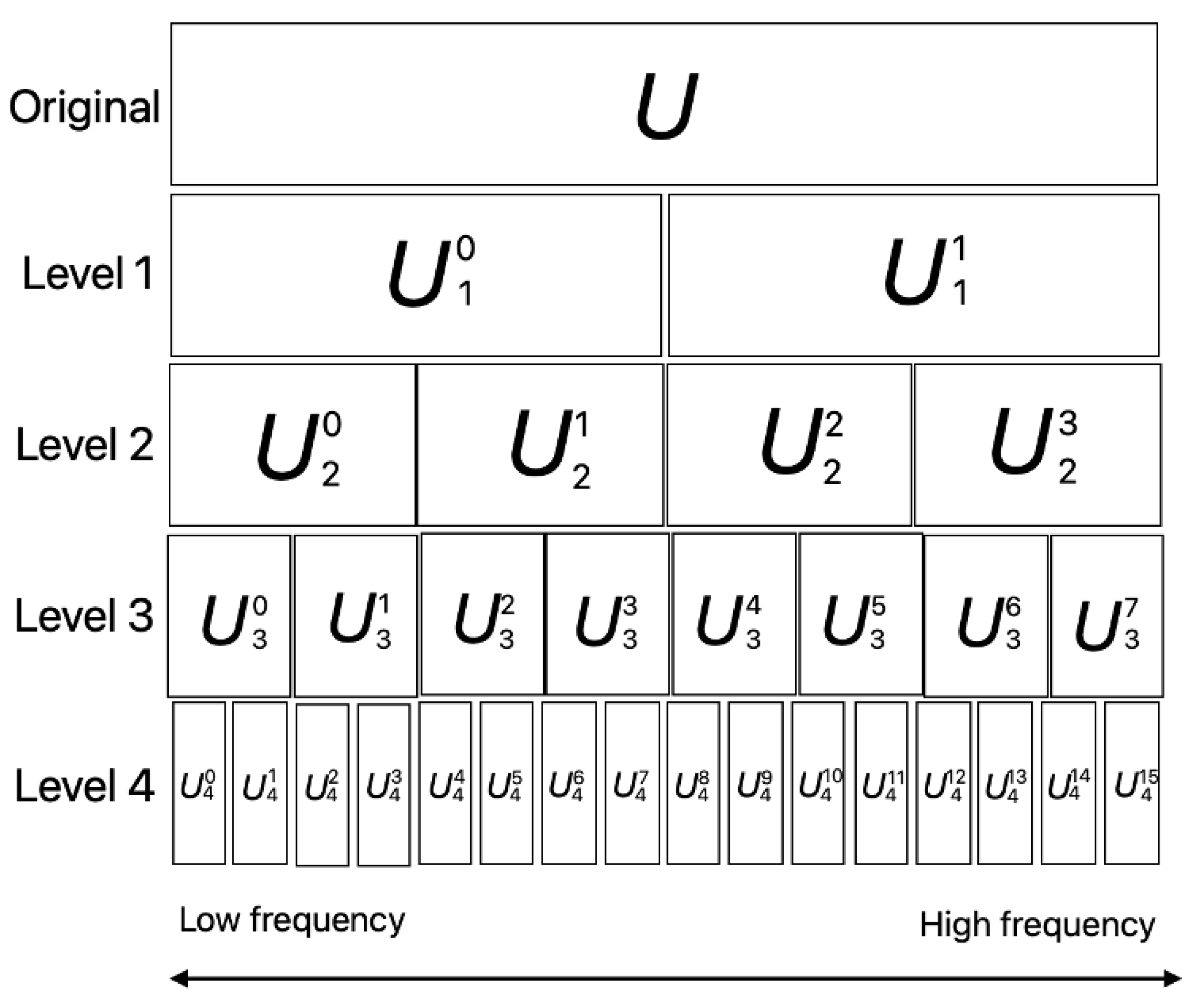
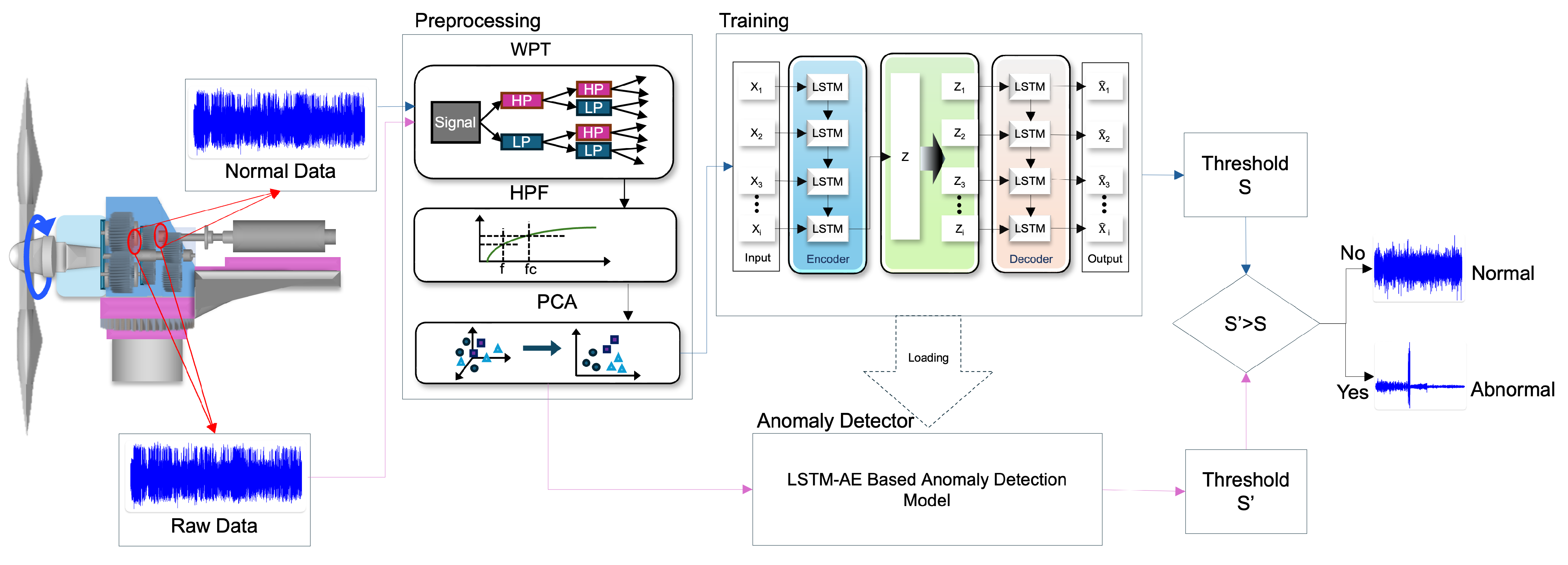
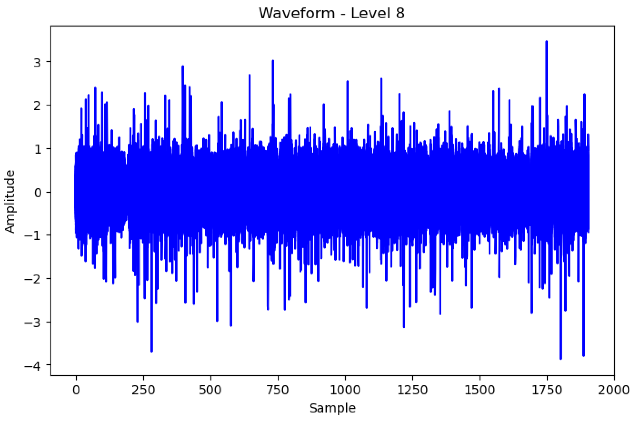
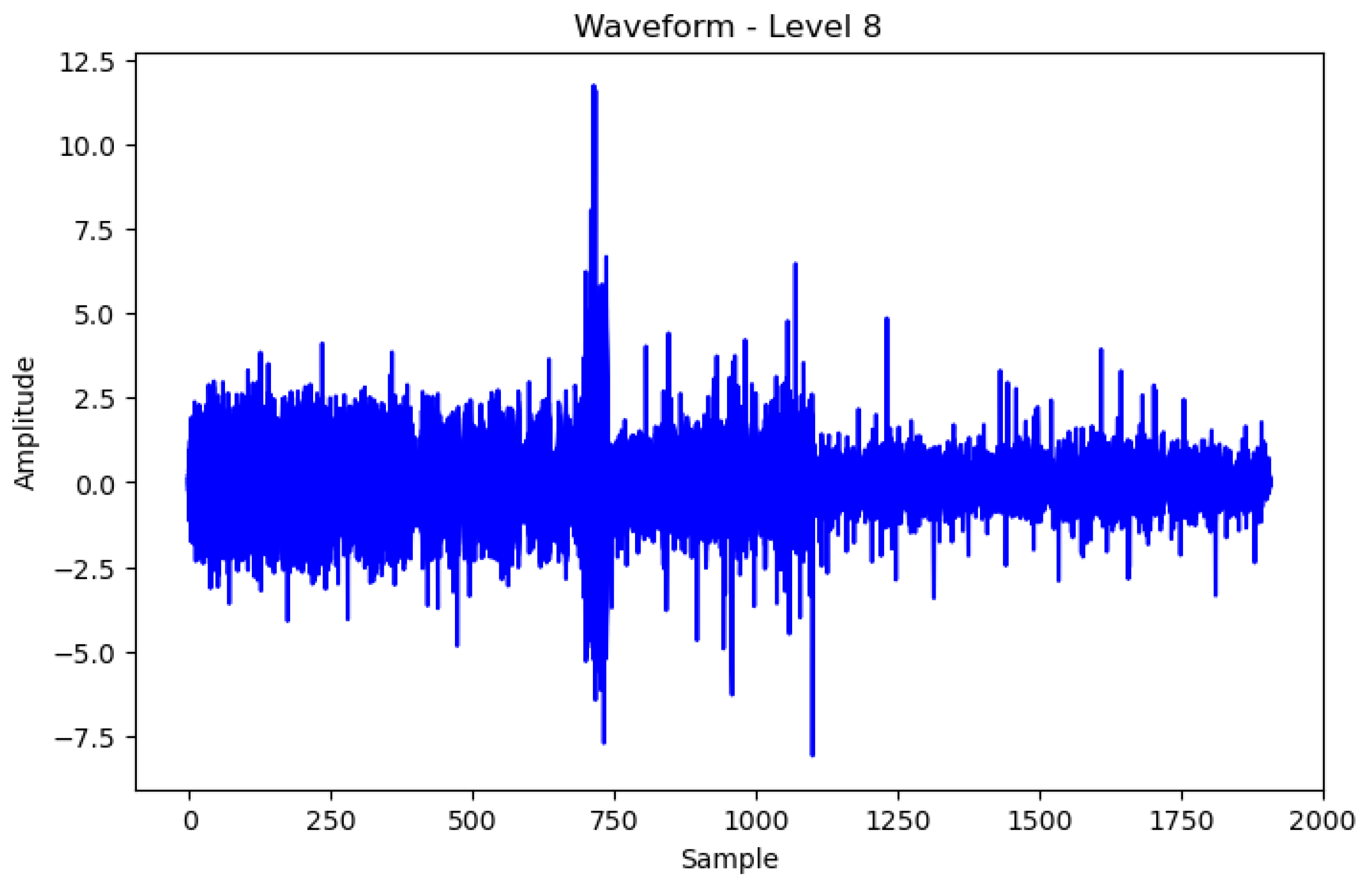
- In this study, we used wavelet packet decomposition to decompose one signal into multiple bandwidth signals and used a high-frequency filter to emphasize the high-frequency part. We used the filtered signal through principal component analysis to benefit from computing resources and analysis through dimensionality reduction.
- When applying the preprocessing method proposed in this study, the reconstruction error of learning and predicting the data by unsupervised learning was about 97%, which was better than the reconstruction error (about 94%) when no preprocessing method was previously applied.
- The preprocessing method proposed in this study has shown that it improves performance even for simple models. The results of this study are expected to be useful in signal and speech processing and will be helpful for new preprocessing methods.
2. Related Work
2.1. Wind Power Generators
2.2. Preprocessing Methods
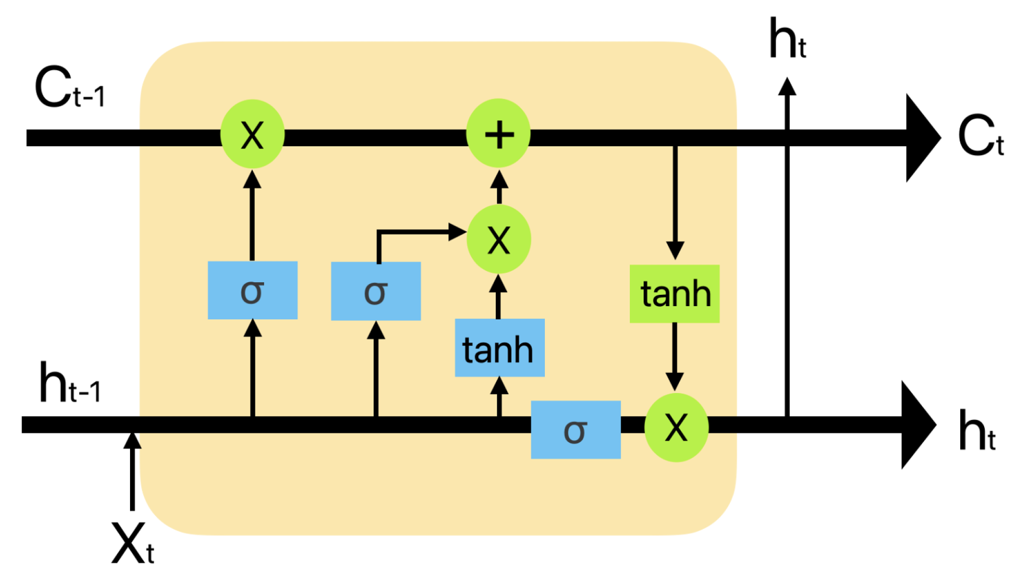
2.3. LSTM
2.4. Anomaly Detection
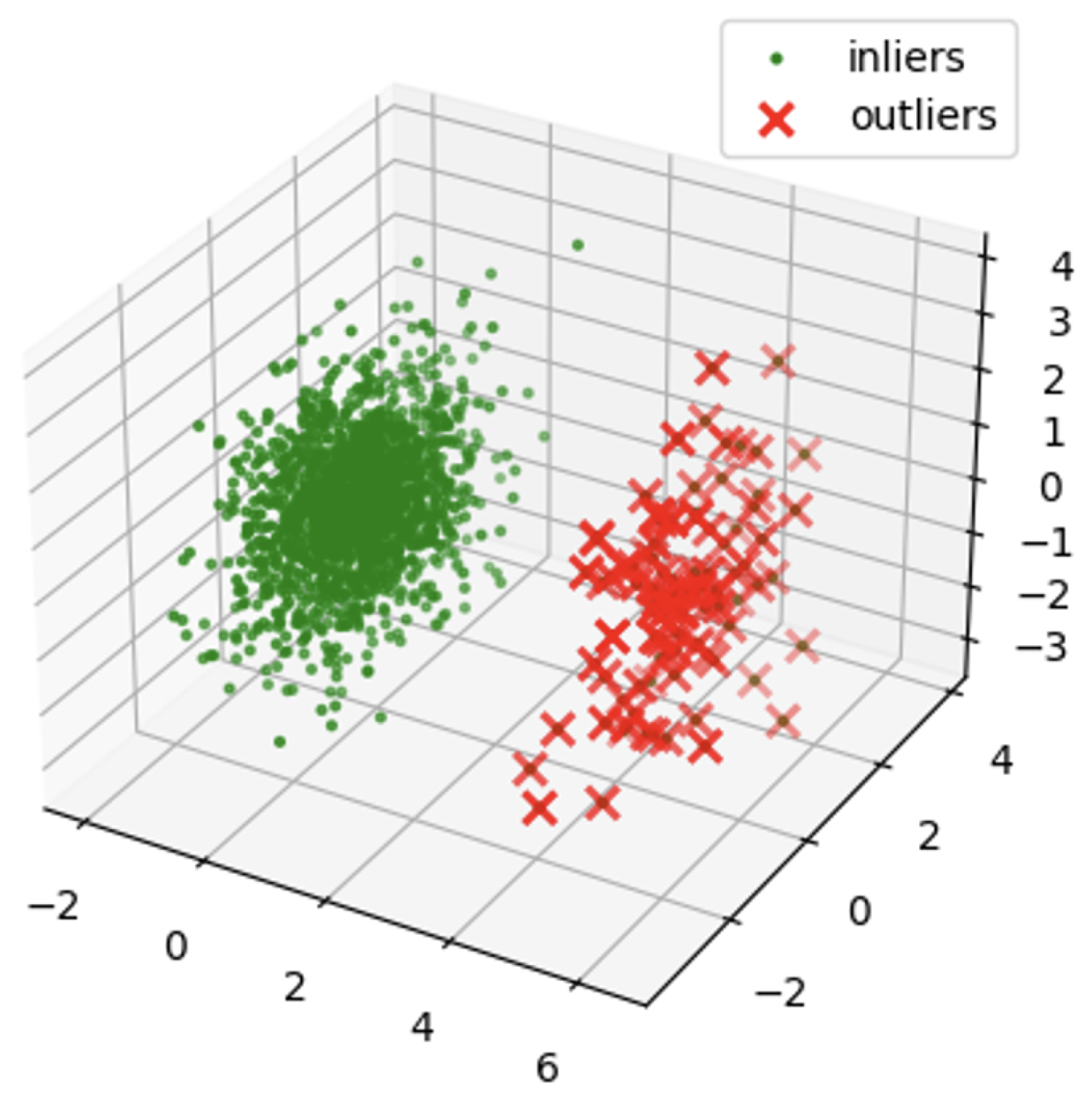
2.5. Isolation Forest
3. LSTM Autoencoder Based Anomaly Detection
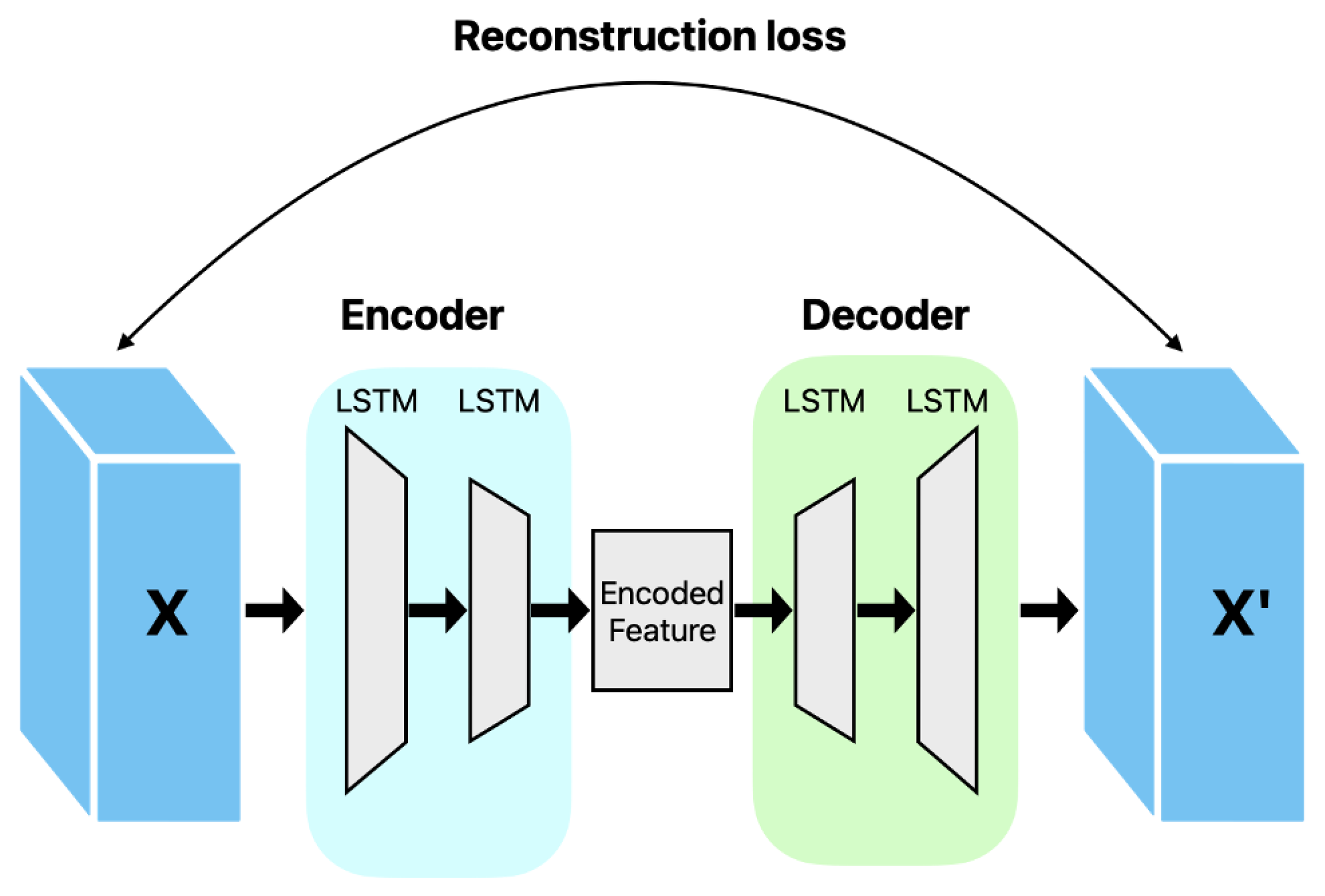
3.1. Model Structure
3.2. Anomaly Detector
3.3. Loss Function
4. Experiment and Results
4.1. Experiment Environments
4.2. Parameter Setting
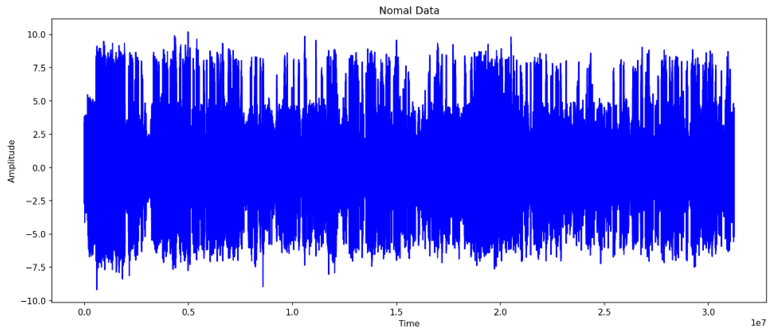
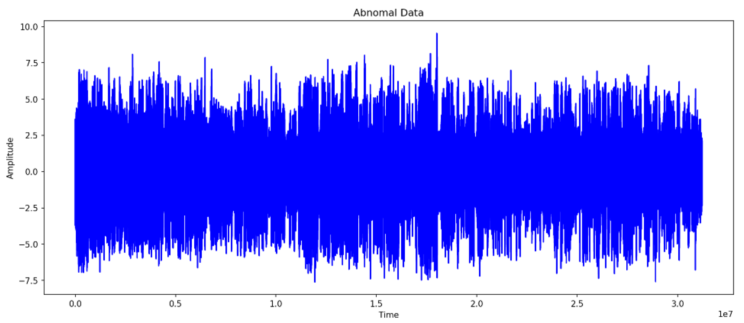
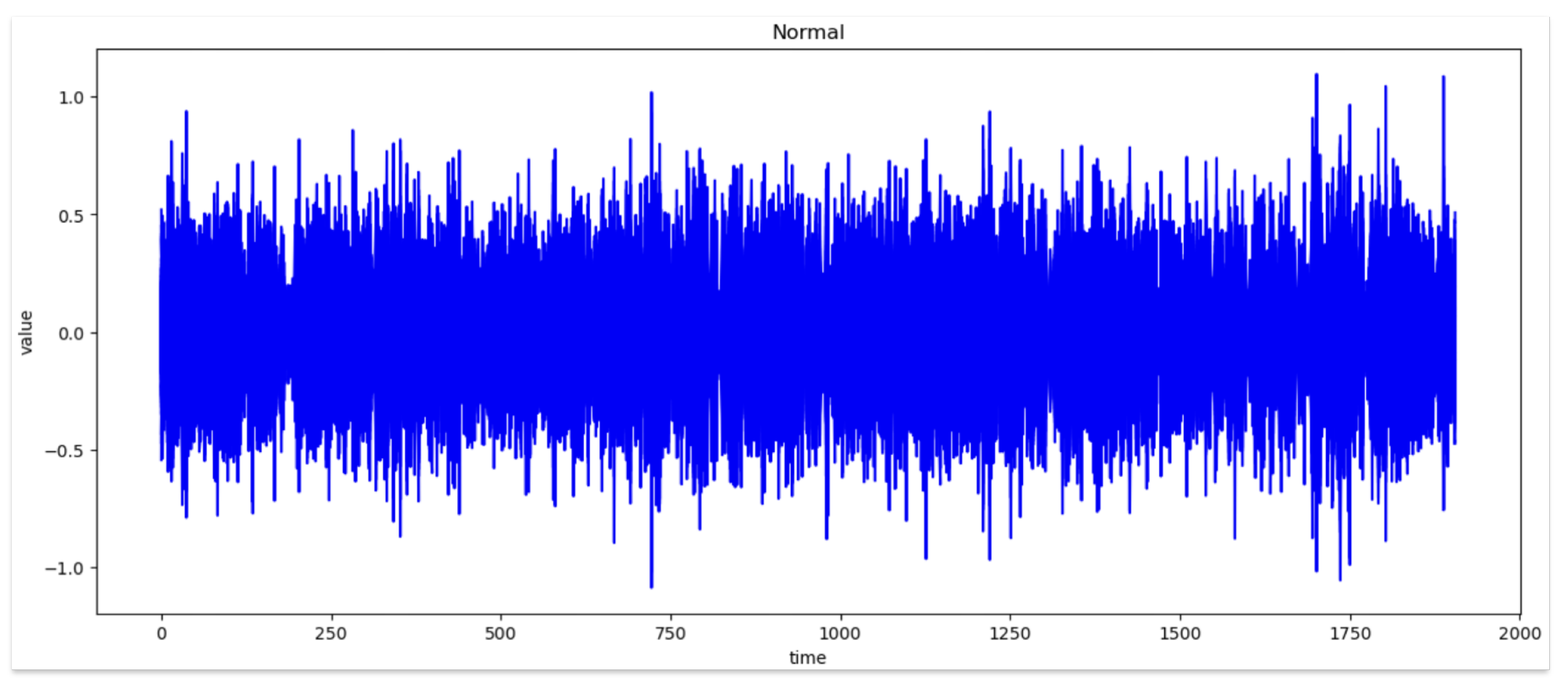
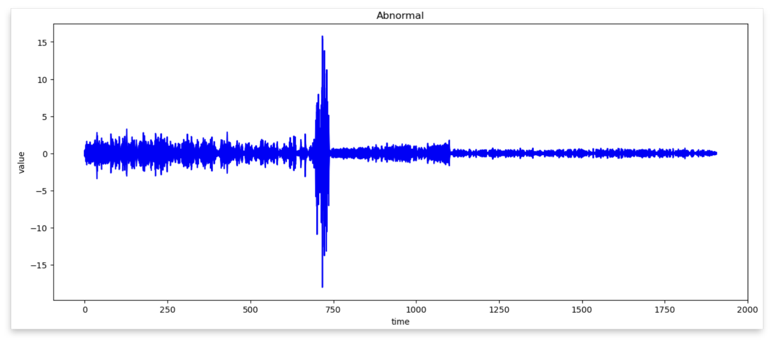
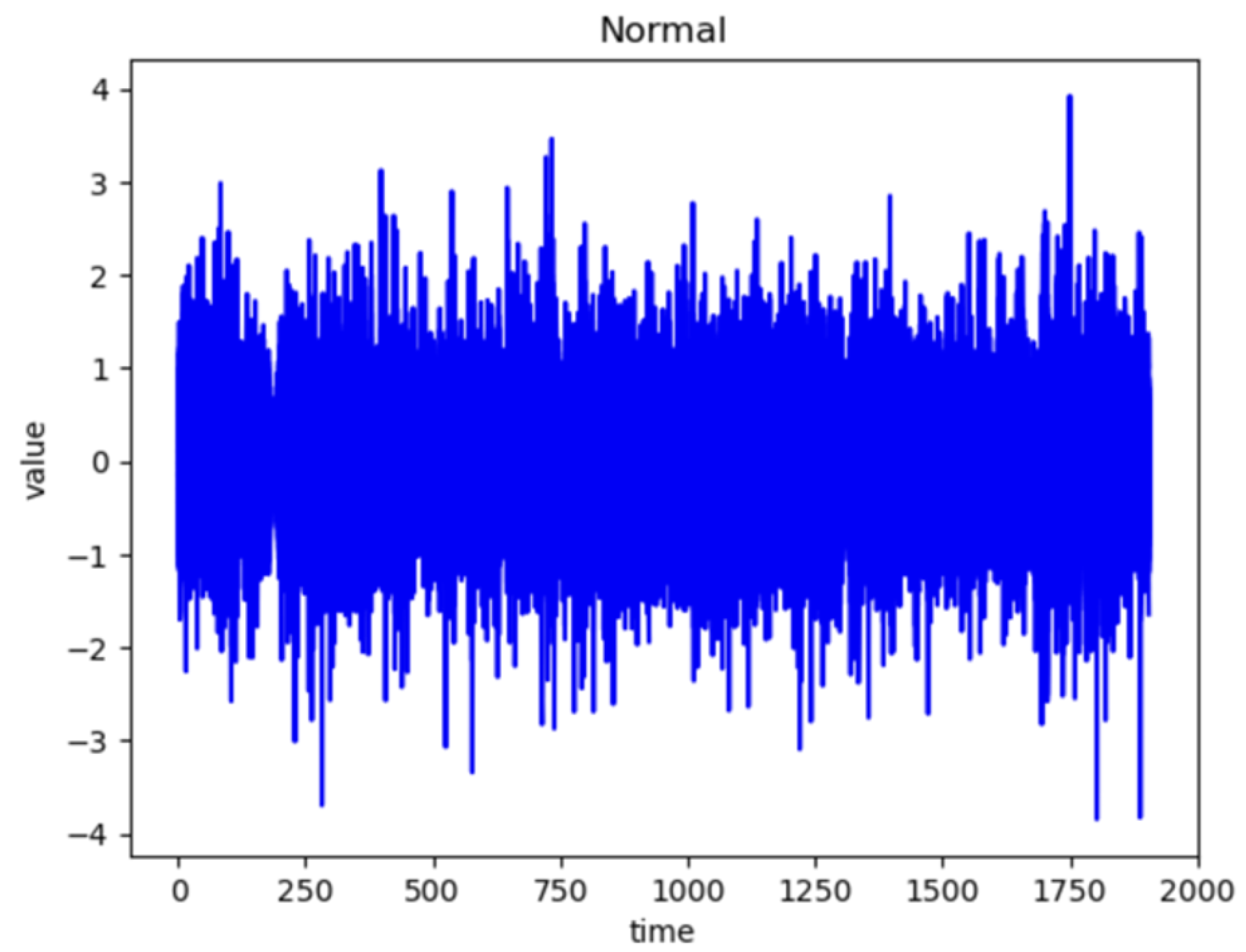
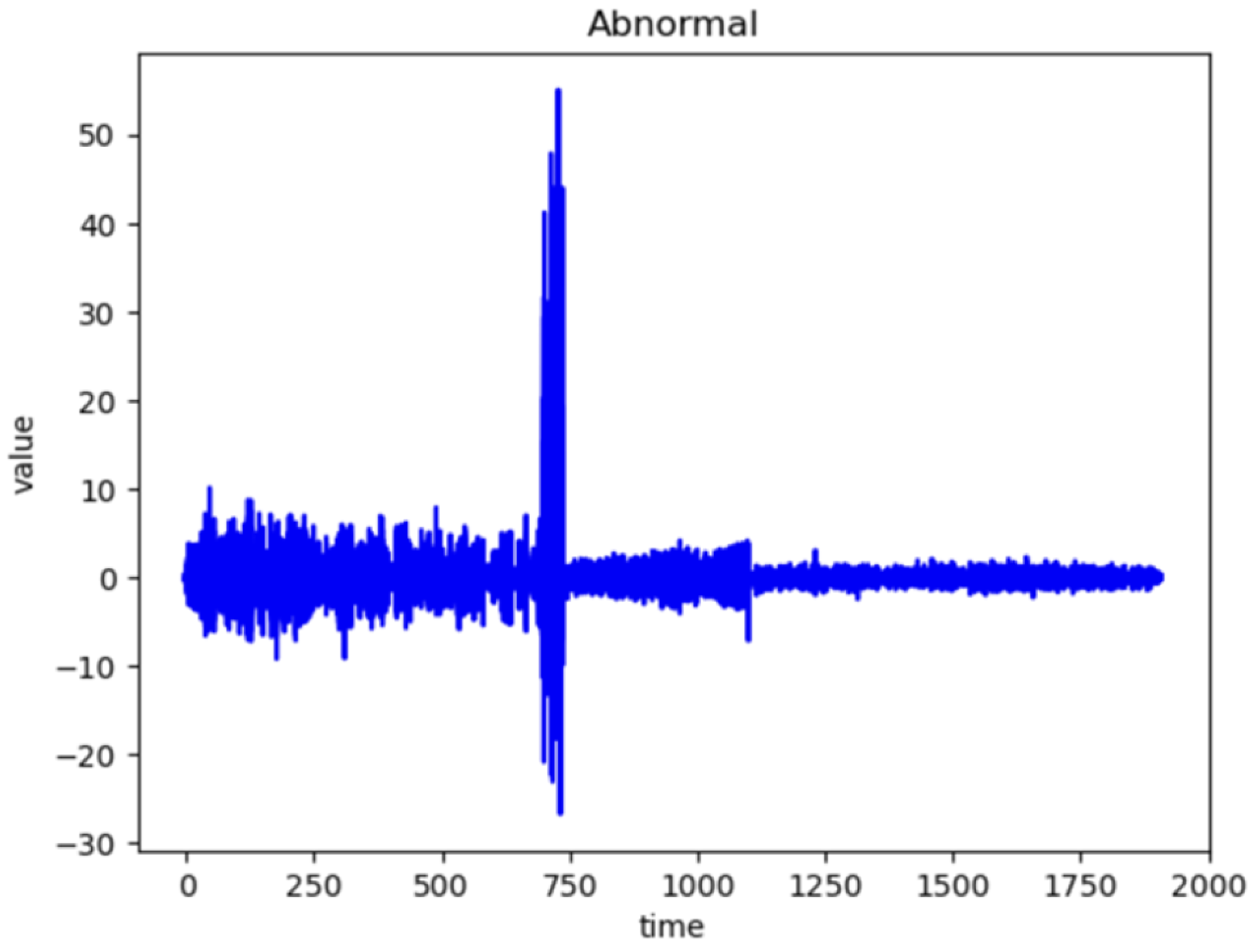
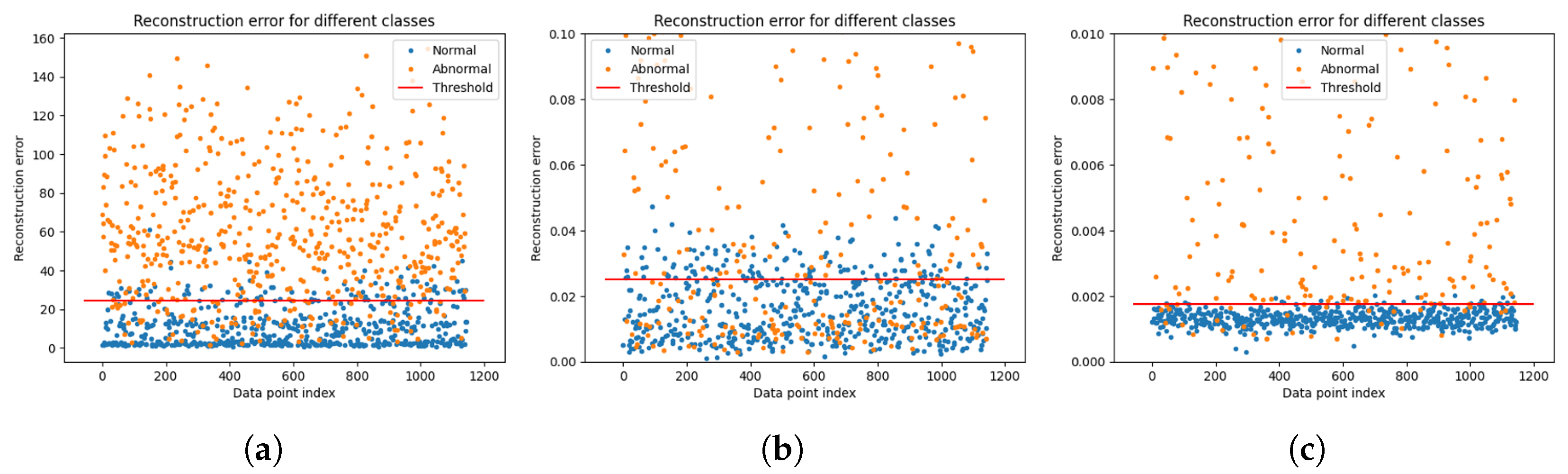
4.3. Comparison of Normal and Abnormal Data
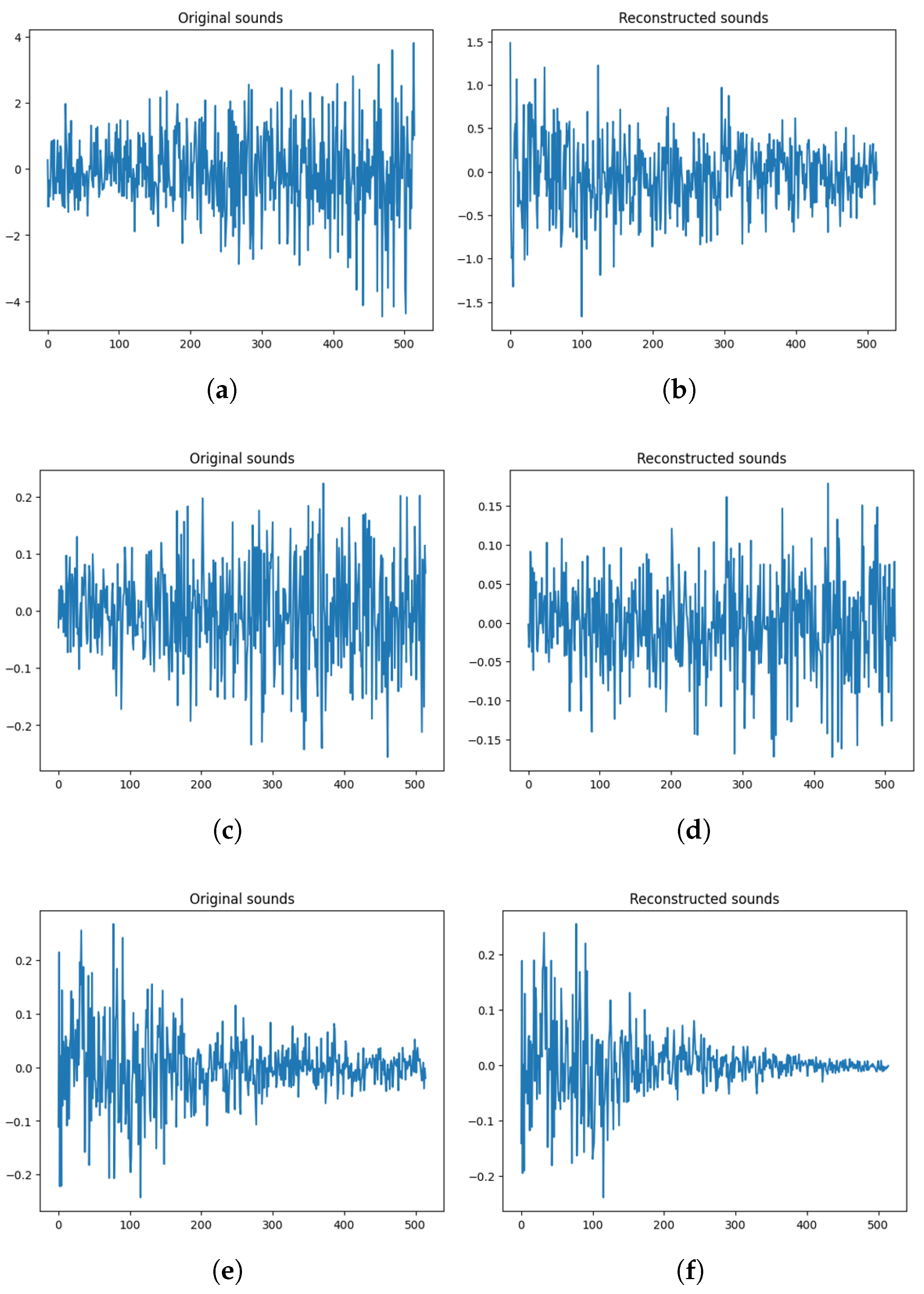
4.4. Results
4.5. Discussion
5. Conclusions
Author Contributions
Funding
Institutional Review Board Statement
Informed Consent Statement
Data Availability Statement
Acknowledgments
Conflicts of Interest
References
- Peng, Z. Modelling and Simulation of Direct Drive Permanent Magnet Wind Power Generation System Based on Simulink. In Proceedings of the IEEE 2021 2nd International Conference on Intelligent Computing and Human-Computer Interaction (ICHCI), Shenyang, China, 17–19 November 2021; pp. 344–350. [Google Scholar]
- Sikiru, S.; Oladosu, T.L.; Amosa, T.I.; Olutoki, J.O.; Ansari, M.; Abioye, K.J.; Rehman, Z.U.; Soleimani, H. Hydrogen-powered horizons: Transformative technologies in clean energy generation, distribution, and storage for sustainable innovation. Int. J. Hydrogen Energy 2024, 56, 1152–1182. [Google Scholar] [CrossRef]
- Ding, X.; Liu, X. Renewable energy development and transportation infrastructure matters for green economic growth? Empirical evidence from China. Econ. Anal. Policy 2023, 79, 634–646. [Google Scholar] [CrossRef]
- Omer, A.M. Energy, environment and sustainable development. Renew. Sustain. Energy Rev. 2008, 12, 2265–2300. [Google Scholar] [CrossRef]
- Nguyen, M.P.; Ponomarenko, T.; Nguyen, N. Energy Transition in Vietnam: A Strategic Analysis and Forecast. Sustainability 2024, 16, 1969. [Google Scholar] [CrossRef]
- Mandal, D.K.; Bose, S.; Biswas, N.; Manna, N.K.; Cuce, E.; Benim, A.C. Solar Chimney Power Plants for Sustainable Air Quality Management Integrating Photocatalysis and Particulate Filtration: A Comprehensive Review. Sustainability 2024, 16, 2334. [Google Scholar] [CrossRef]
- Liang, W.; Liu, W. Key technologies analysis of small scale non-grid-connected wind turbines: A review. In Proceedings of the IEEE 2010 World Non-Grid-Connected Wind Power and Energy Conference, Nanjing, China, 5–7 November 2010; pp. 1–6. [Google Scholar]
- Ackermann, T.; Söder, L. Wind energy technology and current status: A review. Renew. Sustain. Energy Rev. 2000, 4, 315–374. [Google Scholar] [CrossRef]
- Mary, S.A.J.; Sarika, S. Fault Diagnosis and Control Techniques for Wind Energy Conversion System: A Systematic Review. In Proceedings of the IEEE 2022 Third International Conference on Intelligent Computing Instrumentation and Control Technologies (ICICICT), Kannur, India, 11–12 August 2022; pp. 700–704. [Google Scholar]
- Zemali, Z.; Cherroun, L.; Hadroug, N.; Hafaifa, A.; Iratni, A.; Alshammari, O.S.; Colak, I. Robust intelligent fault diagnosis strategy using Kalman observers and neuro-fuzzy systems for a wind turbine benchmark. Renew. Energy 2023, 205, 873–898. [Google Scholar] [CrossRef]
- Chen, J.; Li, J.; Chen, W.; Wang, Y.; Jiang, T. Anomaly detection for wind turbines based on the reconstruction of condition parameters using stacked denoising autoencoders. Renew. Energy 2020, 147, 1469–1480. [Google Scholar] [CrossRef]
- Gupta, S.; Muthiyan, N.; Kumar, S.; Nigam, A.; Dinesh, D.A. A supervised deep learning framework for proactive anomaly detection in cloud workloads. In Proceedings of the 2017 14th IEEE India Council International Conference (INDICON), Roorkee, India, 15–17 December 2017; pp. 1–6. [Google Scholar]
- Lee, M.C.; Lin, J.C.; Gan, E.G. ReRe: A lightweight real-time ready-to-go anomaly detection approach for time series. In Proceedings of the 2020 IEEE 44th Annual Computers, Software, and Applications Conference (COMPSAC), Madrid, Spain, 13–17 July 2020; pp. 322–327. [Google Scholar]
- Wang, Q.; Bu, S.; He, Z. Achieving predictive and proactive maintenance for high-speed railway power equipment with LSTM-RNN. IEEE Trans. Ind. Inform. 2020, 16, 6509–6517. [Google Scholar] [CrossRef]
- Ji, T.; Sivakumar, A.N.; Chowdhary, G.; Driggs-Campbell, K. Proactive anomaly detection for robot navigation with multi-sensor fusion. IEEE Robot. Autom. Lett. 2022, 7, 4975–4982. [Google Scholar] [CrossRef]
- Spantideas, S.; Giannopoulos, A.; Cambeiro, M.A.; Trullols-Cruces, O.; Atxutegi, E.; Trakadas, P. Intelligent Mission Critical Services over Beyond 5G Networks: Control Loop and Proactive Overload Detection. In Proceedings of the IEEE 2023 International Conference on Smart Applications, Communications and Networking (SmartNets), Istanbul, Turkiye, 25–27 July 2023; pp. 1–6. [Google Scholar]
- Huang, D.; Zhang, W.A.; Guo, F.; Liu, W.; Shi, X. Wavelet packet decomposition-based multiscale CNN for fault diagnosis of wind turbine gearbox. IEEE Trans. Cybern. 2021, 53, 443–453. [Google Scholar] [CrossRef] [PubMed]
- Bhandari, B.; Poudel, S.R.; Lee, K.T.; Ahn, S.H. Mathematical modeling of hybrid renewable energy system: A review on small hydro-solar-wind power generation. Int. J. Precis. Eng. Manuf.-Green Technol. 2014, 1, 157–173. [Google Scholar] [CrossRef]
- Jiang, G.; He, H.; Xie, P.; Tang, Y. Stacked multilevel-denoising autoencoders: A new representation learning approach for wind turbine gearbox fault diagnosis. IEEE Trans. Instrum. Meas. 2017, 66, 2391–2402. [Google Scholar] [CrossRef]
- Bengio, Y.; Courville, A.C.; Vincent, P. Unsupervised feature learning and deep learning: A review and new perspectives. CoRR abs/1206.5538 2012, 1, 2012. [Google Scholar]
- Kuzu, A.; Baran, E.A.; Bogosyan, S.; Gokasan, M.; Sabanovic, A. Wavelet packet transform-based compression for teleoperation. Proc. Inst. Mech. Eng. Part I J. Syst. Control. Eng. 2015, 229, 639–651. [Google Scholar] [CrossRef]
- Lotfollahi-Yaghin, M.A.; Koohdaragh, M. Examining the function of wavelet packet transform (WPT) and continues wavelet transform (CWT) in recognizing the crack specification. KSCE J. Civ. Eng. 2011, 15, 497–506. [Google Scholar] [CrossRef]
- Prieto, M.; Novo, B.; Manzanedo, F. The Wavelet Packet Transform and its application to identify arc furnace current and voltage harmonics. In Proceedings of the 2008 IEEE Canada Electric Power Conference, Vancouver, BC, Canada, 6–7 October 2008; pp. 1–6. [Google Scholar]
- Stein, S.A.M.; Loccisano, A.E.; Firestine, S.M.; Evanseck, J.D. Principal components analysis: A review of its application on molecular dynamics data. Annu. Rep. Comput. Chem. 2006, 2, 233–261. [Google Scholar]
- Babu, P.A.; Prasad, K. Removal of ocular artifacts from EEG signals by fast RLS algorithm using wavelet transform. Int. J. Comput. Appl. 2011, 21, 1–5. [Google Scholar] [CrossRef]
- Magid, S.A.; Zhang, Y.; Wei, D.; Jang, W.D.; Lin, Z.; Fu, Y.; Pfister, H. Dynamic high-pass filtering and multi-spectral attention for image super-resolution. In Proceedings of the IEEE/CVF International Conference on Computer Vision, Montreal, BC, Canada, 11–17 October 2021; pp. 4288–4297. [Google Scholar]
- Kiakojouri, A.; Lu, Z.; Mirring, P.; Powrie, H.; Wang, L. A Novel Hybrid Technique Combining Improved Cepstrum Pre-Whitening and High-Pass Filtering for Effective Bearing Fault Diagnosis Using Vibration Data. Sensors 2023, 23, 9048. [Google Scholar] [CrossRef]
- Moharm, K.; Eltahan, M.; Elsaadany, E. Wind speed forecast using LSTM and Bi-LSTM algorithms over gabal El-Zayt wind farm. In Proceedings of the IEEE 2020 International Conference on Smart Grids and Energy Systems (SGES), Perth, Australia, 23–26 November 2020; pp. 922–927. [Google Scholar]
- Nguyen, H.D.; Tran, K.P.; Thomassey, S.; Hamad, M. Forecasting and Anomaly Detection approaches using LSTM and LSTM Autoencoder techniques with the applications in supply chain management. Int. J. Inf. Manag. 2021, 57, 102282. [Google Scholar] [CrossRef]
- Sagheer, A.; Kotb, M. Unsupervised pre-training of a deep LSTM-based stacked autoencoder for multivariate time series forecasting problems. Sci. Rep. 2019, 9, 19038. [Google Scholar] [CrossRef] [PubMed]
- Park, D.; Hoshi, Y.; Kemp, C.C. A multimodal anomaly detector for robot-assisted feeding using an lstm-based variational autoencoder. IEEE Robot. Autom. Lett. 2018, 3, 1544–1551. [Google Scholar] [CrossRef]
- Geiger, A.; Liu, D.; Alnegheimish, S.; Cuesta-Infante, A.; Veeramachaneni, K. Tadgan: Time series anomaly detection using generative adversarial networks. In Proceedings of the 2020 IEEE International Conference on Big Data (Big Data), Atlanta, GA, USA, 10–13 December 2020; pp. 33–43. [Google Scholar]
- Chen, H.; Liu, H.; Chu, X.; Liu, Q.; Xue, D. Anomaly detection and critical SCADA parameters identification for wind turbines based on LSTM-AE neural network. Renew. Energy 2021, 172, 829–840. [Google Scholar] [CrossRef]
- Said Elsayed, M.; Le-Khac, N.A.; Dev, S.; Jurcut, A.D. Network anomaly detection using LSTM based autoencoder. In Proceedings of the 16th ACM Symposium on QoS and Security for Wireless and Mobile Networks, Alicante, Spain, 16–20 November 2020; pp. 37–45. [Google Scholar]
- Goldstein, M.; Uchida, S. A comparative evaluation of unsupervised anomaly detection algorithms for multivariate data. PLoS ONE 2016, 11, e0152173. [Google Scholar] [CrossRef] [PubMed]
- Aggarwal, C.C.; Yu, P.S. Outlier detection for high dimensional data. In Proceedings of the 2001 ACM SIGMOD International Conference on Management of Data, Santa Barbara, CA, USA, 21–24 May 2001; pp. 37–46. [Google Scholar]
- Xiang, G.; Min, W. Applying Semi-supervised cluster algorithm for anomaly detection. In Proceedings of the IEEE 2010 Third International Symposium on Information Processing, Qingdao, China, 15–17 October 2010; pp. 43–45. [Google Scholar]
- Kiran, B.R.; Thomas, D.M.; Parakkal, R. An overview of deep learning based methods for unsupervised and semi-supervised anomaly detection in videos. J. Imaging 2018, 4, 36. [Google Scholar] [CrossRef]
- Lashgari, E.; Liang, D.; Maoz, U. Data augmentation for deep-learning-based electroencephalography. J. Neurosci. Methods 2020, 346, 108885. [Google Scholar] [CrossRef] [PubMed]
- Wulsin, D.; Gupta, J.; Mani, R.; Blanco, J.; Litt, B. Modeling electroencephalography waveforms with semi-supervised deep belief nets: Fast classification and anomaly measurement. J. Neural Eng. 2011, 8, 036015. [Google Scholar] [CrossRef] [PubMed]
- Manevitz, L.M.; Yousef, M. One-class SVMs for document classification. J. Mach. Learn. Res. 2001, 2, 139–154. [Google Scholar]
- Längkvist, M.; Karlsson, L.; Loutfi, A. A review of unsupervised feature learning and deep learning for time-series modeling. Pattern Recognit. Lett. 2014, 42, 11–24. [Google Scholar] [CrossRef]
- Li, J.L.; Zhou, Y.F.; Ying, Z.Y.; Xu, H.; Li, Y.; Li, X. Anomaly Detection Based on Isolated Forests. In Proceedings of the Advances in Artificial Intelligence and Security: 7th International Conference, ICAIS 2021, Dublin, Ireland, 19–23 July 2021; pp. 486–495. [Google Scholar]
- Liu, F.T.; Ting, K.M.; Zhou, Z.H. Isolation forest. In Proceedings of the 2008 Eighth IEEE International Conference on Data Mining, Pisa, Italy, 15–19 December 2008; pp. 413–422. [Google Scholar]
- He, K.; Li, X. Time–frequency feature extraction of acoustic emission signals in aluminum alloy MIG welding process based on SST and PCA. IEEE Access 2019, 7, 113988–113998. [Google Scholar] [CrossRef]
- Xiang, S.; Qin, Y.; Zhu, C.; Wang, Y.; Chen, H. LSTM networks based on attention ordered neurons for gear remaining life prediction. ISA Trans. 2020, 106, 343–354. [Google Scholar] [CrossRef] [PubMed]
- Xu, X.; Yoneda, M. Multitask air-quality prediction based on LSTM-autoencoder model. IEEE Trans. Cybern. 2019, 51, 2577–2586. [Google Scholar] [CrossRef] [PubMed]
- Yan, H.; Liu, Z.; Chen, J.; Feng, Y.; Wang, J. Memory-augmented skip-connected autoencoder for unsupervised anomaly detection of rocket engines with multi-source fusion. ISA Trans. 2023, 133, 53–65. [Google Scholar] [CrossRef] [PubMed]
- Ferris, M.H.; McLaughlin, M.; Grieggs, S.; Ezekiel, S.; Blasch, E.; Alford, M.; Cornacchia, M.; Bubalo, A. Using ROC curves and AUC to evaluate performance of no-reference image fusion metrics. In Proceedings of the IEEE 2015 National Aerospace and Electronics Conference (NAECON), Dayton, OH, USA, 15–19 June 2015; pp. 27–34. [Google Scholar]
- Priyanto, C.Y.; Hendry; Purnomo, H.D. Combination of Isolation Forest and LSTM Autoencoder for Anomaly Detection. In Proceedings of the 2021 2nd International Conference on Innovative and Creative Information Technology (ICITech), Salatiga, Indonesia, 23–25 September 2021; pp. 35–38. [Google Scholar] [CrossRef]
- Martin-del Campo, S.; Sandin, F.; Strömbergsson, D. Dictionary learning approach to monitoring of wind turbine drivetrain bearings. arXiv 2019, arXiv:1902.01426. [Google Scholar] [CrossRef]
- Maleki, S.; Maleki, S.; Jennings, N.R. Unsupervised anomaly detection with LSTM autoencoders using statistical data-filtering. Appl. Soft Comput. 2021, 108, 107443. [Google Scholar] [CrossRef]


| Normal Data | Abnormal Data | |
|---|---|---|
| Components = 515 | 0.9890 | 0.9856 |
| PCA Data | HPF-PCA Data | WPT-HPF-PCA Data | |
|---|---|---|---|
| Epoch 30 | 35.0556 | 0.1078 | 0.0065 |
| Epoch 60 | 24.8907 | 0.0604 | 0.0029 |
| Epoch 90 | 18.6556 | 0.0333 | 0.0021 |
| Epoch 120 | 14.2359 | 0.0220 | 0.0017 |
| Epoch 150 | 11.7810 | 0.0181 | 0.0015 |
| PCA | HPF-PCA | WPT-HPF-PCA | |
|---|---|---|---|
| AUC | 0.9410 | 0.8622 | 0.9744 |
Disclaimer/Publisher’s Note: The statements, opinions and data contained in all publications are solely those of the individual author(s) and contributor(s) and not of MDPI and/or the editor(s). MDPI and/or the editor(s) disclaim responsibility for any injury to people or property resulting from any ideas, methods, instructions or products referred to in the content. |
© 2024 by the authors. Licensee MDPI, Basel, Switzerland. This article is an open access article distributed under the terms and conditions of the Creative Commons Attribution (CC BY) license (https://creativecommons.org/licenses/by/4.0/).
Share and Cite
Lee, Y.; Park, C.; Kim, N.; Ahn, J.; Jeong, J. LSTM-Autoencoder Based Anomaly Detection Using Vibration Data of Wind Turbines. Sensors 2024, 24, 2833. https://doi.org/10.3390/s24092833
Lee Y, Park C, Kim N, Ahn J, Jeong J. LSTM-Autoencoder Based Anomaly Detection Using Vibration Data of Wind Turbines. Sensors. 2024; 24(9):2833. https://doi.org/10.3390/s24092833
Chicago/Turabian StyleLee, Younjeong, Chanho Park, Namji Kim, Jisu Ahn, and Jongpil Jeong. 2024. "LSTM-Autoencoder Based Anomaly Detection Using Vibration Data of Wind Turbines" Sensors 24, no. 9: 2833. https://doi.org/10.3390/s24092833
APA StyleLee, Y., Park, C., Kim, N., Ahn, J., & Jeong, J. (2024). LSTM-Autoencoder Based Anomaly Detection Using Vibration Data of Wind Turbines. Sensors, 24(9), 2833. https://doi.org/10.3390/s24092833