

A Hybrid Soft Sensor Model for Measuring the Oxygen Content in Boiler Flue Gas

Abstract
1. Introduction
- (1)
- The prediction of the oxygen content in flue gas typically involves multiple variables, which often have noise and redundant information present in the actual data. By using PCA, the high-dimensional dataset can be transformed into a lower-dimensional one, thereby enhancing the computational efficiency and accuracy of the soft measurement method. By utilizing Pearson’s method for selecting auxiliary variables and combining it with PCA, it is possible to transform high-dimensional datasets into low-dimensional ones. Additionally, the implementation of the 3σ criteria and smooth curve methods can effectively eliminate abnormal data, resulting in enhanced computational efficiency and accuracy in soft sensing.
- (2)
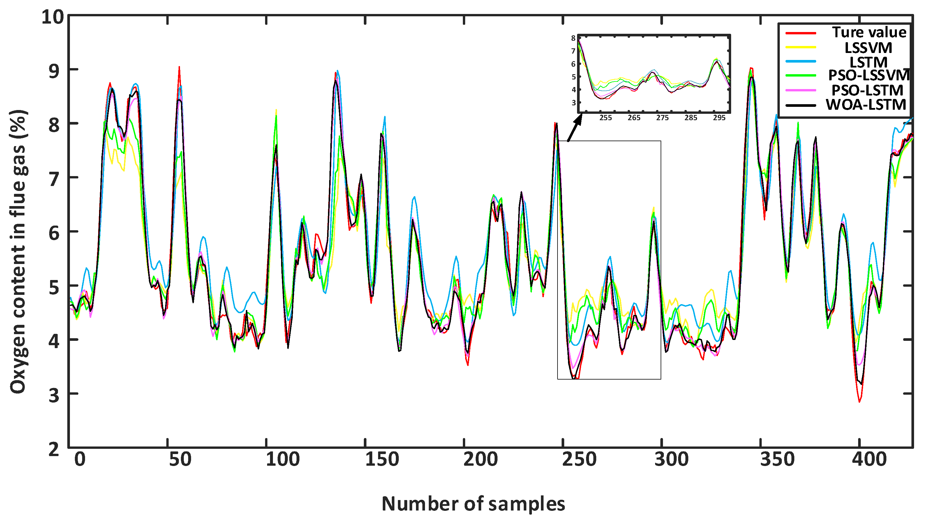
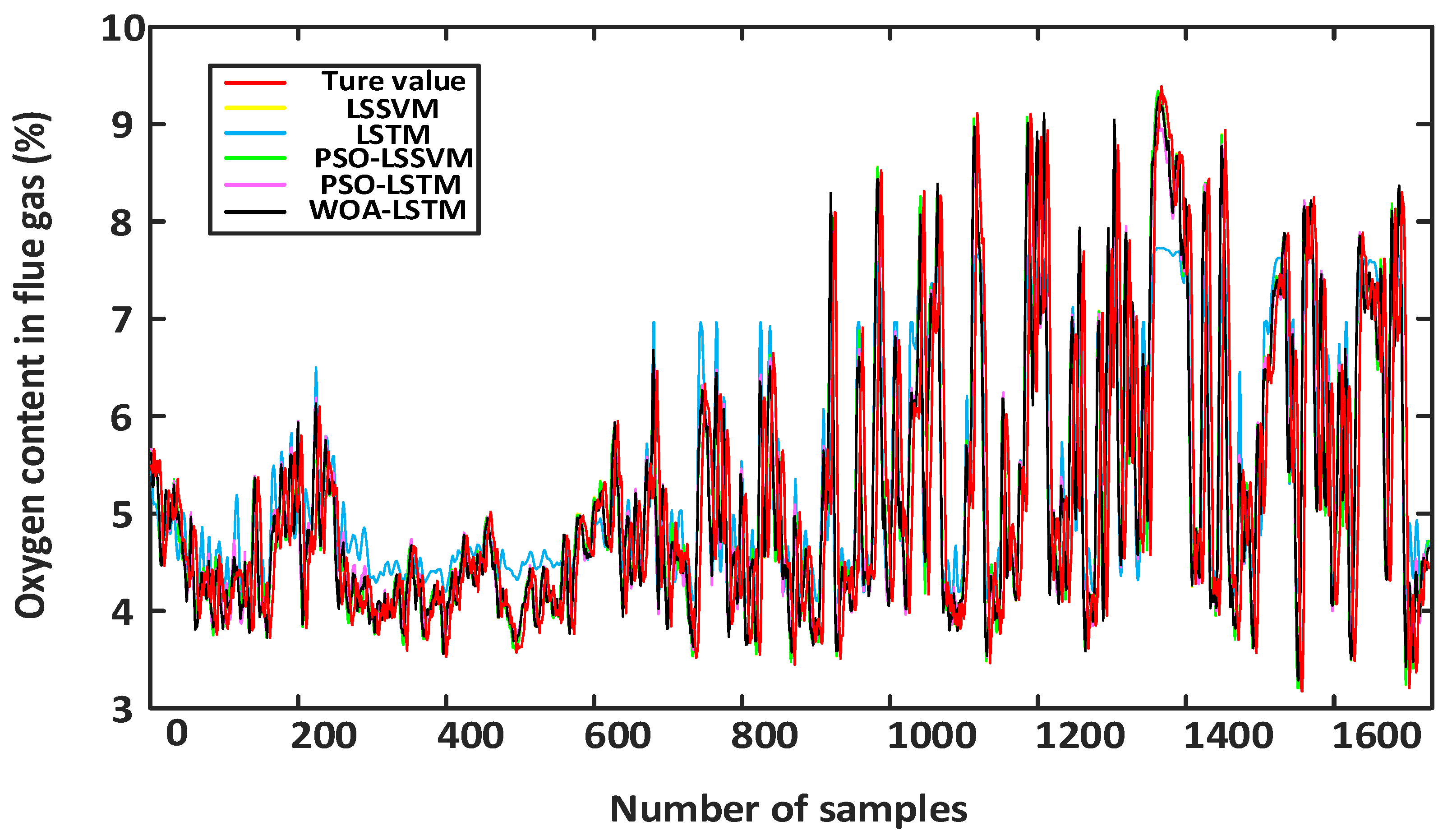
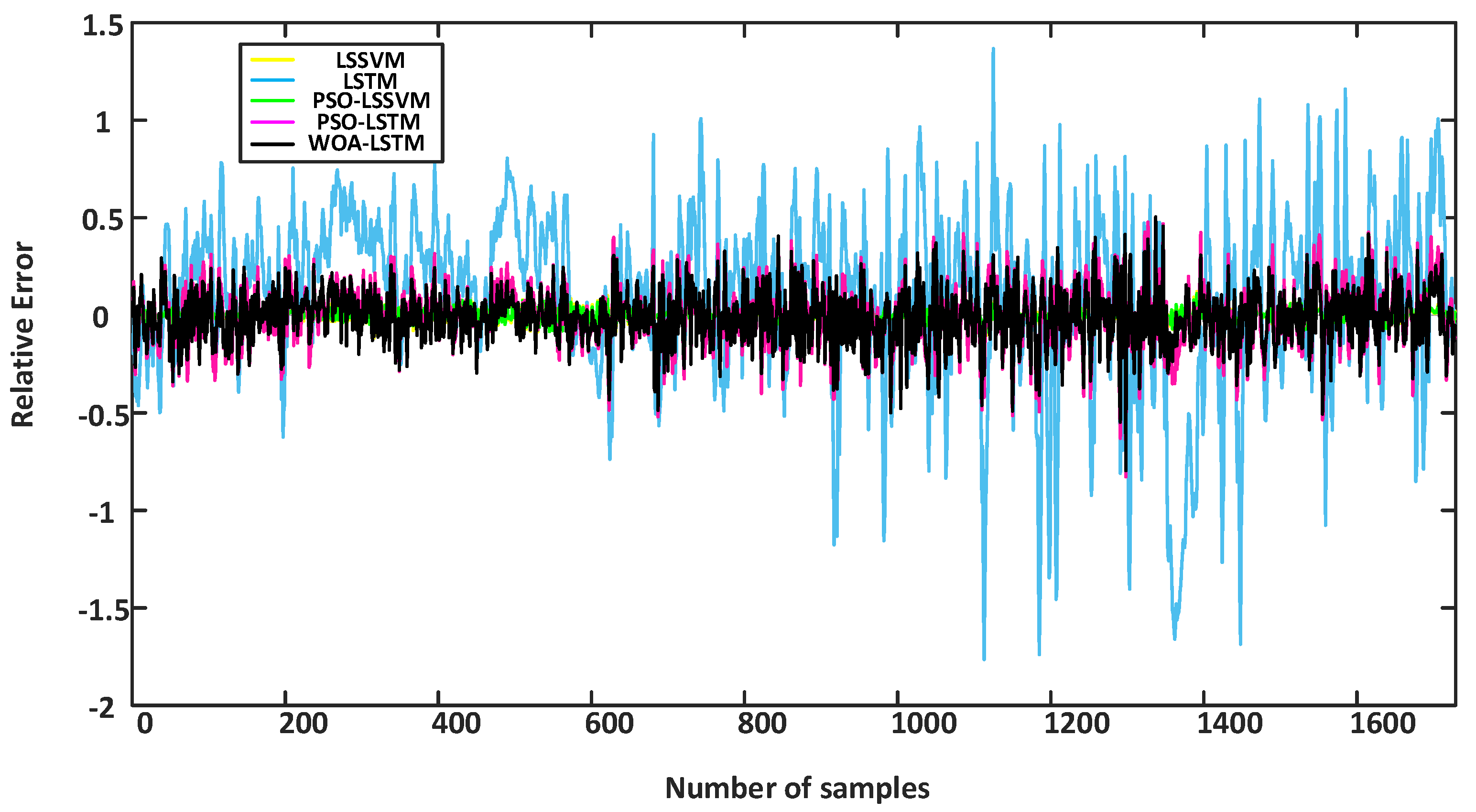
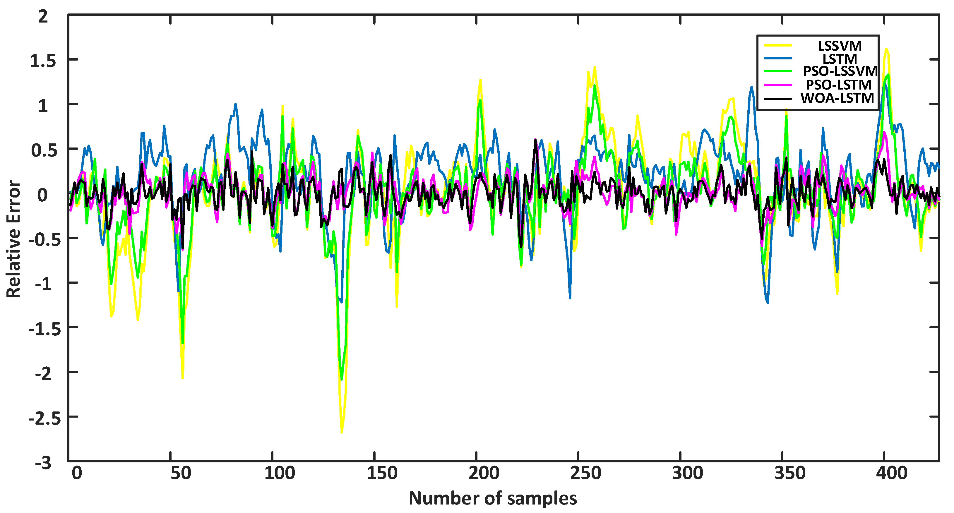
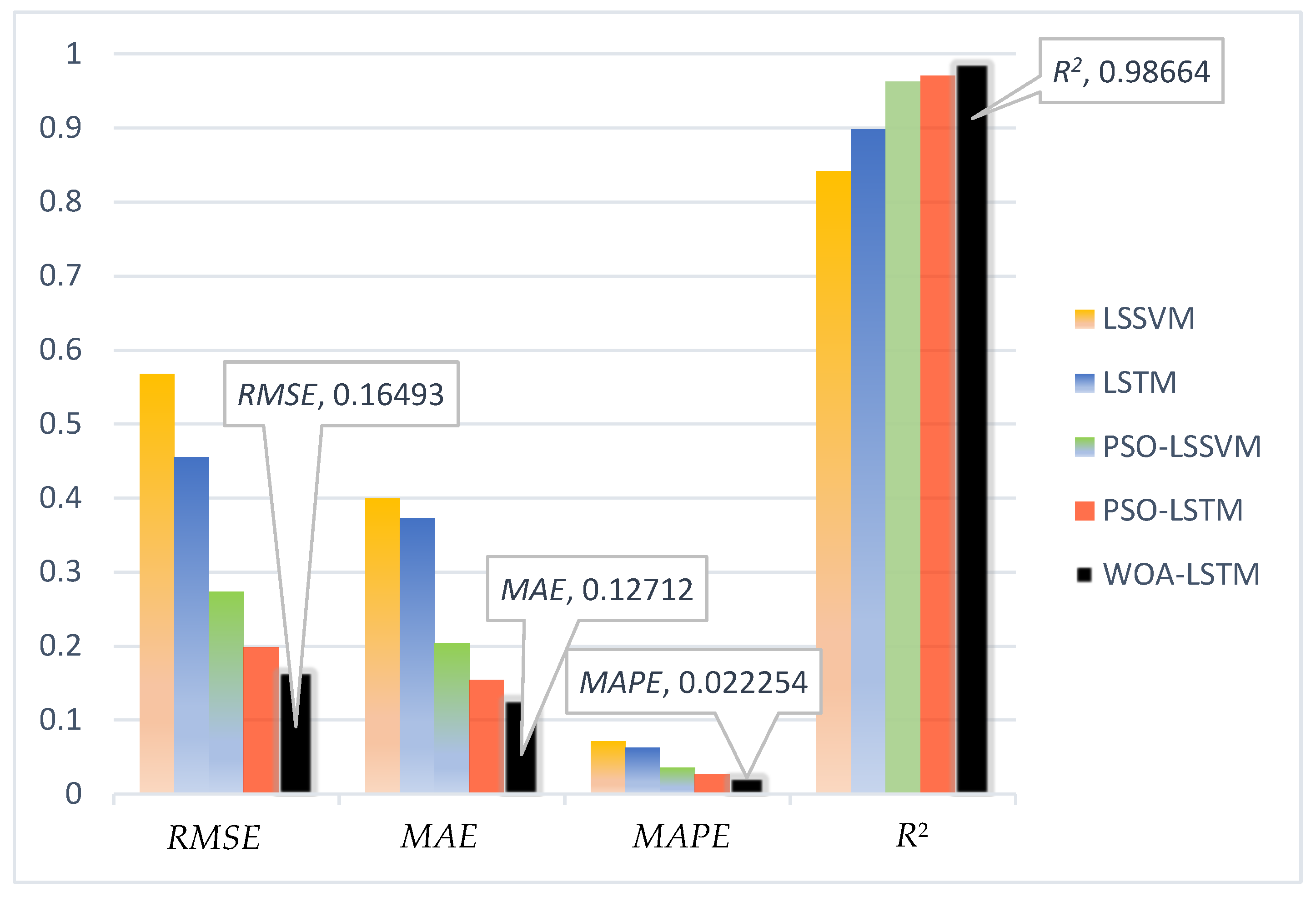
- To the extent of our knowledge, there is a relatively limited amount of research on the use of the WOA-LSTM hybrid model for predicting the oxygen content in flue gases in soft sensor applications. To improve the precision of the LSTM model in predicting the oxygen content in flue gas, the study used the WOA optimizing the learning rate, hidden layer units, and regularization coefficient of the LSTM model. Compared with the LSTM, LSSVM, PSO-LSTM, and PSO-LSSVM models, the WOA-LSTM model achieved a high level of predictive accuracy for the oxygen content in the flue gas.
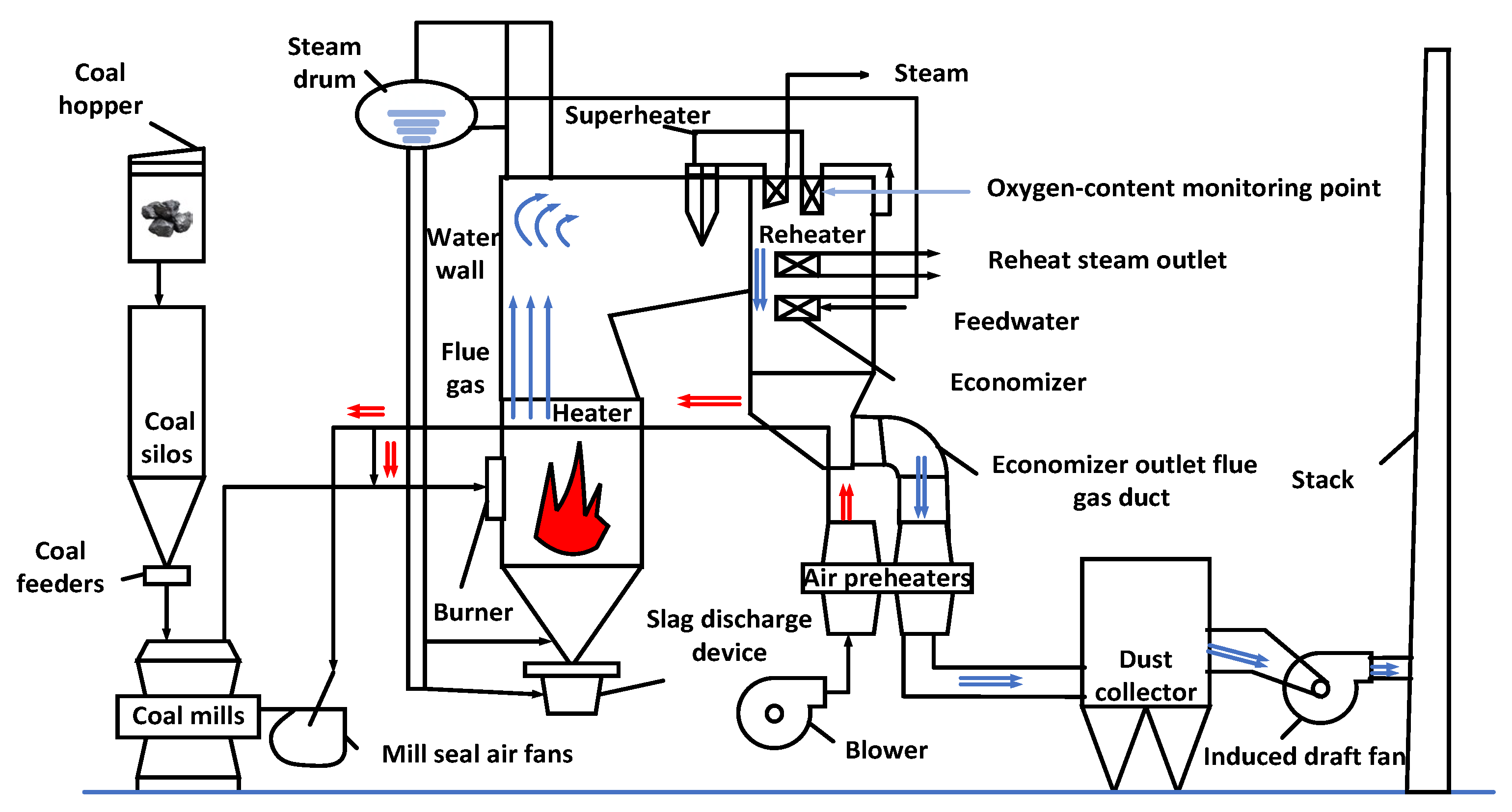
2. Analysis of the Coal-Fired Boiler System
3. Theoretical Foundations
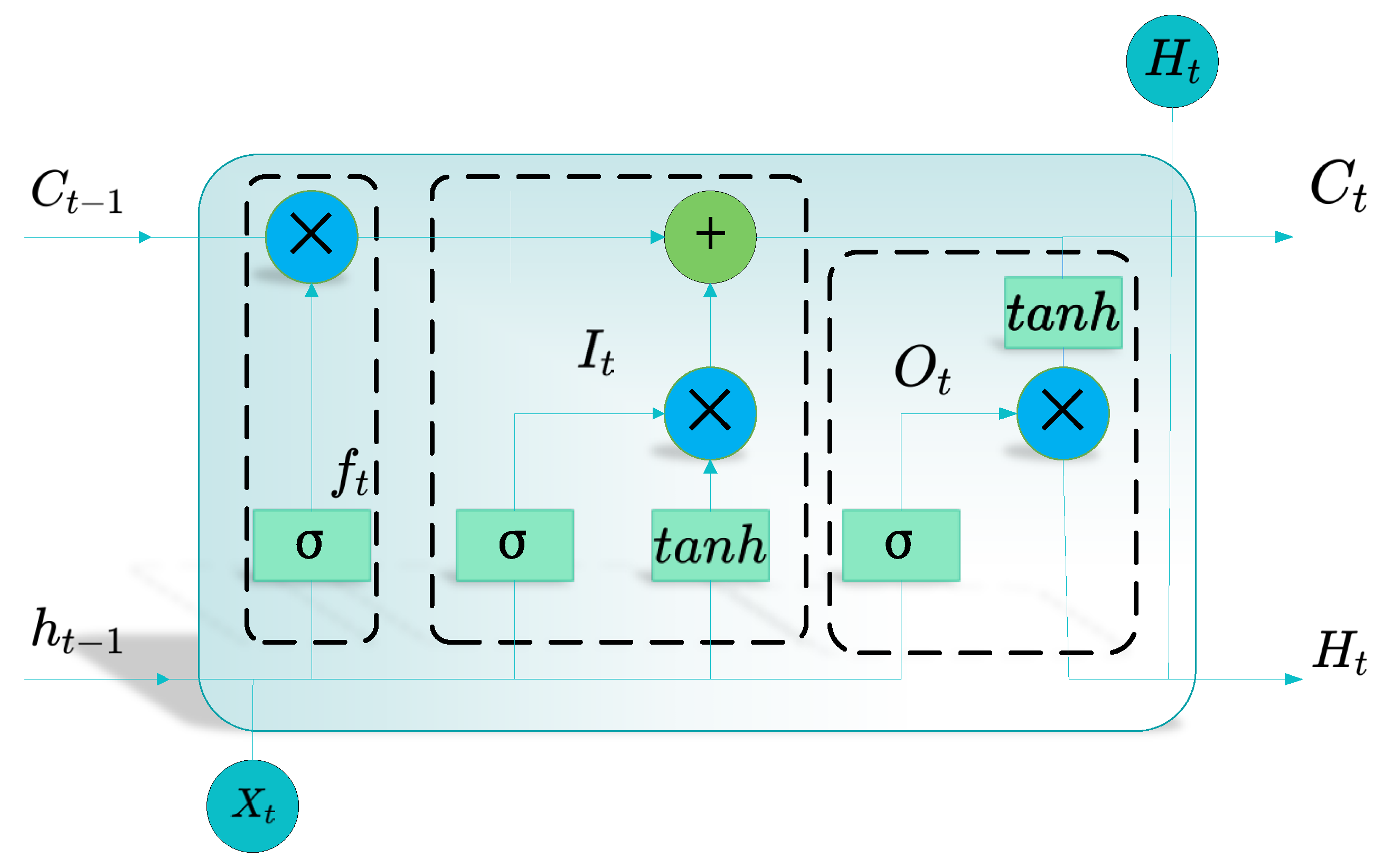
3.1. LSTM Model of the Oxygen Content in the Flue Gas
- Forget gate
- Input gate
- State of the cell
- Output gate
3.2. The Whale Optimization Algorithm
- (1)
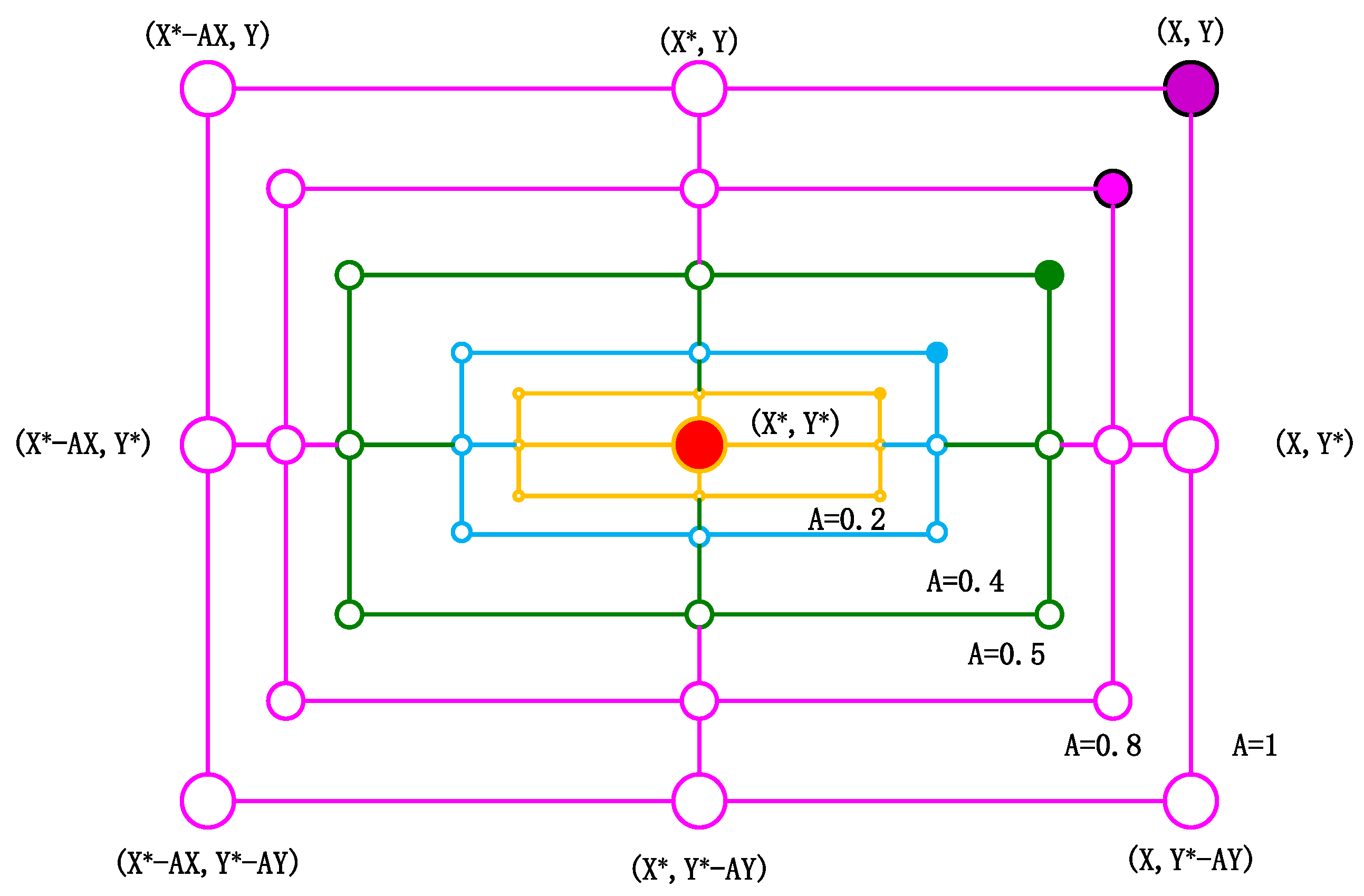
- Encircling prey
- (2)
- Bubble-net attack method
- (3)
- Searching for prey
3.3. WOA-LSTM
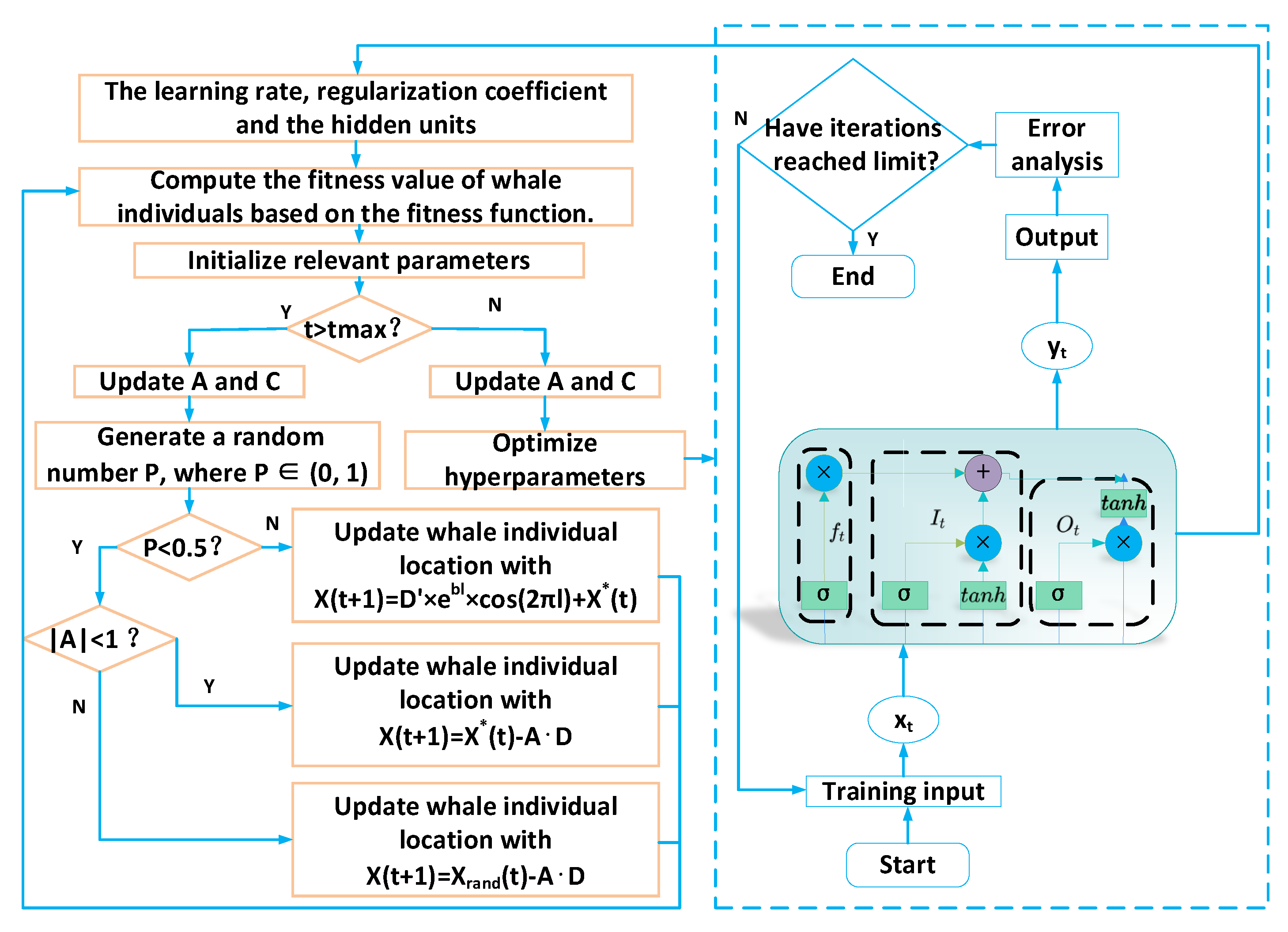
- (a)
- The relevant parameters of the LSTM are initialized, which include the learning rate, the regularization coefficient, and the hidden units.
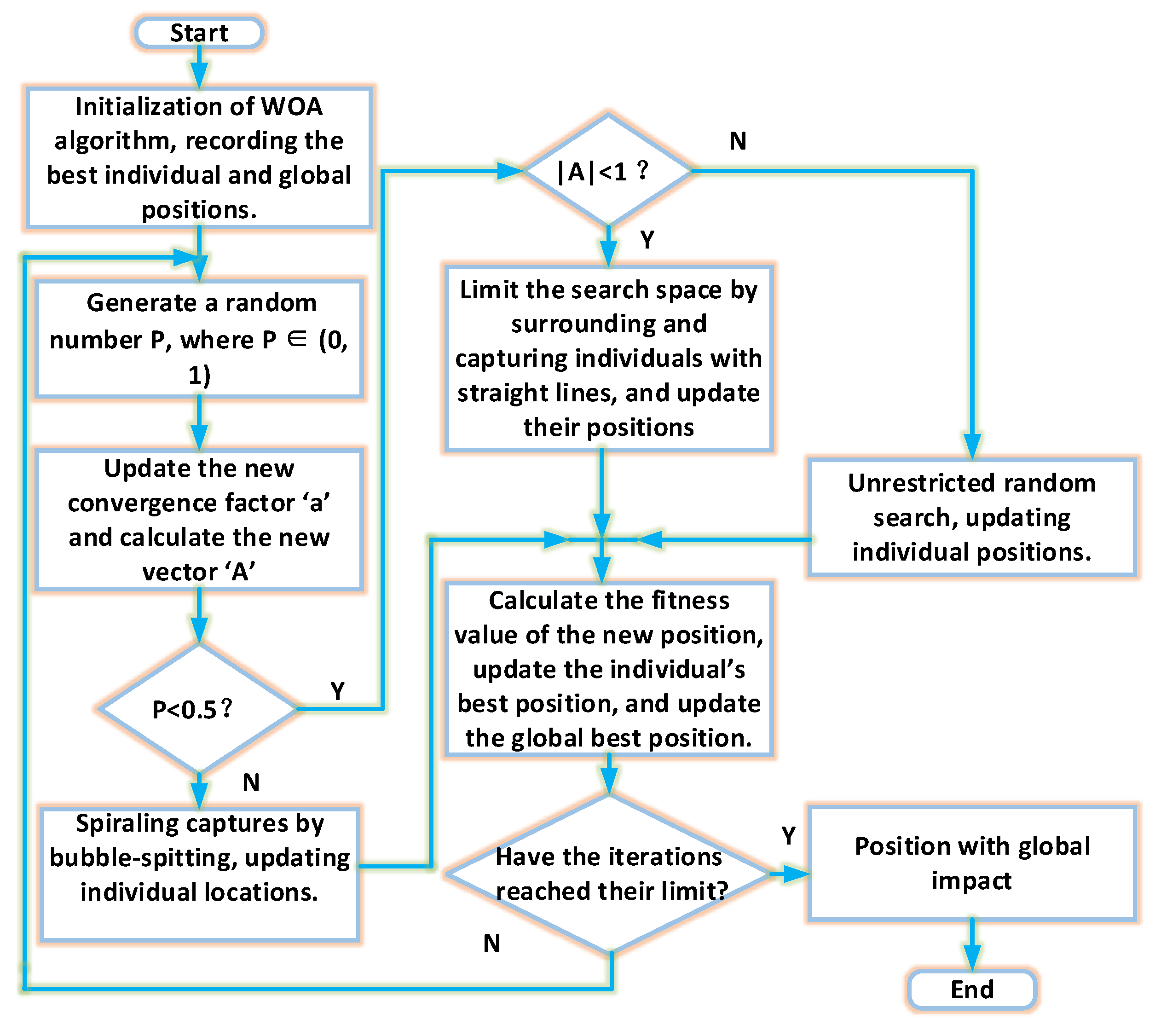
- (b)
- The parameters of the whale optimization algorithm are initialized, which include the maximum number of iterations tmax, the number of whales n, the upper limit of the search range ub, and the lower limit lb.
- (c)
- Compute the fitness of each whale, identify the current optimal whale’s position, and retain it.
- (d)
- Update the coefficient vectors A and C. If the probability P is less than 50%, proceed to the next step; if not, use the mechanism of bubble-net feeding.
- (e)
- If the absolute value of the coefficient vector A is smaller than 1, surround the prey; otherwise, the prey is searched for globally and randomly.
- (f)
- The WOA continuously optimizes the network’s parameters until the iterations end, obtaining the optimal learning rate, the number of neurons in the hidden layer of the neural network, and the regularization coefficient.
- (g)
- Based on the best combination of parameters, output the soft sensing value of the oxygen content in the flue gas.
4. Influencing Attributes of the Output of the Oxygen Content of Flue Gas
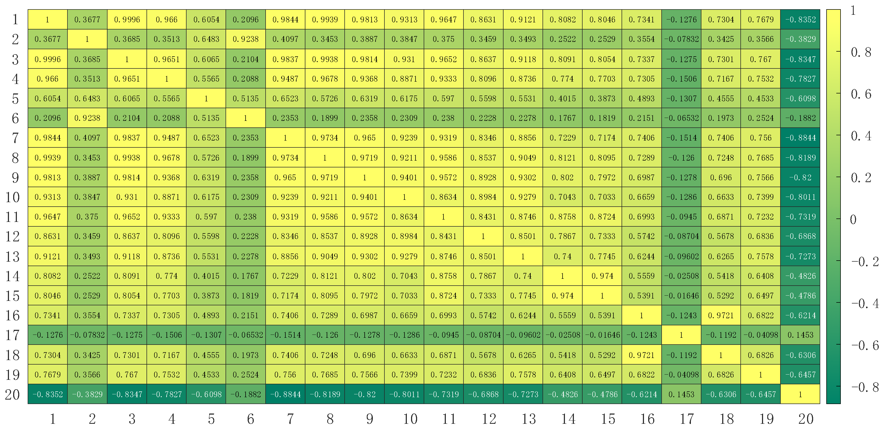
4.1. Pearson’s Correlation
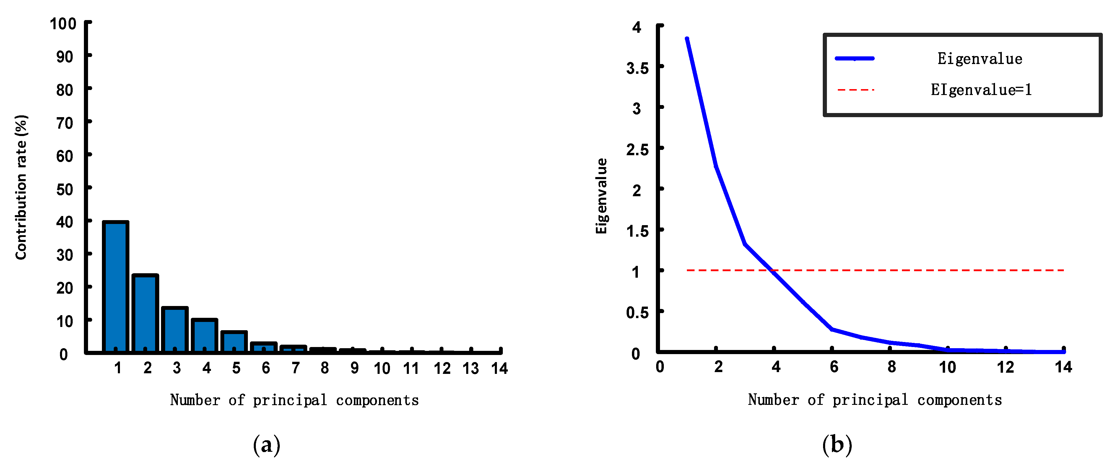
4.2. Principal Component Analysis (PCA)
- (1)
- Structure the entire historical dataset of the load into a sample matrix with the dimensions m n
- (2)
- Compute the mean value of the n-dimensional dataset A, wherewhere m is the total number of samples, and is the obtained sample mean.
- (3)
- Calculate the covariance matrix of the sample set using the generated sample mean.where is the covariance matrix of the sample set.
- (4)
- Calculate the eigenvectors and eigenvalues of the covariance matrixwhere is the diagonal matrix of n eigenvalues arranged in descending order in the covariance matrix, is the eigenvalue corresponding to the covariance matrix, and the feature matrix Q is composed of the feature vectors corresponding to the eigenvalues .
- (5)
- Calculate the cumulative contribution to variance of the top k principal components by using the obtained eigenvalues and eigenvectorswhere is k-th eigenvalue, and p presents the number of variables.
- (6)
- By projecting the original data into a k-dimensional subspace and selecting the top k eigenvectors of the covariance matrix, a new basis for the data is constructed.
4.3. Preprocessing of Data
5. Simulation Results
5.1. Evaluation Indicators
5.2. Experimental Results
5.3. Experimental Analysis and Comparison
6. Conclusions
Author Contributions
Funding
Institutional Review Board Statement
Informed Consent Statement
Data Availability Statement
Acknowledgments
Conflicts of Interest
References
- Zhang, W.; Zhang, Y.; Bai, X.; Liu, J.; Zeng, D.; Qiu, T. A Robust Fuzzy Tree Method with Outlier Detection for Combustion Models and Optimization. Chemom. Intell. Lab. Syst. 2016, 158, 130–137. [Google Scholar] [CrossRef]
- Han, X.; Yan, Y.; Cheng, C.; Chen, Y.; Zhu, Y. Monitoring of oxygen content in the flue gas at a coal-fired power plant using cloud modeling techniques. IEEE Trans. Instrum. Meas. 2013, 63, 953–963. [Google Scholar] [CrossRef]
- Liu, Y.; Chen, J.; Sun, Z.; Li, Y.; Huang, D. A Probabilistic Self-Validating Soft-Sensor with Application to Wastewater Treatment. Comput. Chem. Eng. 2014, 71, 263–280. [Google Scholar] [CrossRef]
- Guo, Y.; Zhao, Y.; Huang, B. Development of Soft Sensor by Incorporating the Delayed Infrequent and Irregular Measurements. J. Process Control. 2014, 24, 1733–17396. [Google Scholar] [CrossRef]
- Willett, M. Oxygen Sensing for Industrial Safety—Evolution and New Approaches. Sensors 2014, 14, 6084–6103. [Google Scholar] [CrossRef] [PubMed]
- Yan, W.; Tang, D.; Lin, Y. A Data-Driven Soft Sensor Modeling Method Based on Deep Learning and Its Application. IEEE Trans. Ind. Electron. 2016, 64, 4237–4245. [Google Scholar] [CrossRef]
- Shakil, M.; Elshafei, M.; Habib, M.A.; Maleki, F.A. Soft Sensor for NOx and O2 Using Dynamic Neural Networks. Comput. Electr. Eng. 2009, 35, 578–586. [Google Scholar] [CrossRef]
- Kadlec, P.; Gabrys, B.; Strandt, S. Data-Driven Soft Sensors in the Process Industry. Comput. Chem. Eng. 2009, 33, 795–814. [Google Scholar] [CrossRef]
- Grbić, R.; Slišković, D.; Kadlec, P. Adaptive Soft Sensor for Online Prediction and Process Monitoring Based on a Mixture of Gaussian Process Models. Comput. Chem. Eng. 2013, 58, 84–97. [Google Scholar] [CrossRef]
- Ammiche, M.; Kouadri, A.; Bensmail, A. A Modified Moving Window Dynamic PCA with Fuzzy Logic Filter and Application to Fault Detection. Chemom. Intell. Lab. Syst. 2018, 177, 100–113. [Google Scholar] [CrossRef]
- Bo, L.; Wang, L.; Jiao, L. Recursive Finite Newton Algorithm for Support Vector Regression in the Primal. Neural Comput. 2007, 19, 1082–1096. [Google Scholar] [CrossRef]
- Gonzaga, J.C.B.; Meleiro, L.A.C.; Kiang, C.; Maciel Filho, R. ANN-Based Soft-Sensor for Real-Time Process Monitoring and Control of an Industrial Polymerization Process. Comput. Chem. Eng. 2009, 33, 43–49. [Google Scholar] [CrossRef]
- Chen, J.; Chan, L.L.T.; Cheng, Y.-C. Gaussian Process Regression Based Optimal Design of Combustion Systems Using Flame Images. Appl. Energy 2013, 111, 153–160. [Google Scholar] [CrossRef]
- Lingfang, S.; Yechi, W. Soft-Sensing of Oxygen Content of Flue Gas Based on Mixed Model. Energy Procedia 2012, 17, 221–226. [Google Scholar] [CrossRef]
- Chen, X.; Wang, J. A Soft-Sensing Model for Oxygen-Content in Flue Gases of Coal-Fired Power Plant Based on Neural Network. In Proceedings of the 2018 37th Chinese Control Conference (CCC), Wuhan, China, 25–27 July 2018; IEEE: Piscataway, NJ, USA, 2018; pp. 3657–3661. [Google Scholar]
- Tang, Z.; Zhang, H.; Yang, H. Artificial Neural Networks Model for Predicting Oxygen Content in Flue Gas of Power Plant. In Proceedings of the 2017 29th Chinese Control And Decision Conference (CCDC), Chongqing, China, 28–30 May 2017; IEEE: Piscataway, NJ, USA, 2017; pp. 1379–1382. [Google Scholar]
- Kurniawan, E.D.; Effendy, N.; Arif, A.; Dwiantoro, K.; Muddin, N. Soft Sensor for the Prediction of Oxygen Content in Boiler Flue Gas Using Neural Networks and Extreme Gradient Boosting. Neural Comput. Applic. 2023, 35, 345–352. [Google Scholar] [CrossRef]
- Liu, W. A Survey of Deep Neural Network Architectures and Their Applications. Neurocomputing 2017, 234, 11–26. [Google Scholar] [CrossRef]
- Wang, Y.; Li, X. Soft Measurement for VFA Concentration in Anaerobic Digestion for Treating Kitchen Waste Based on Improved DBN. IEEE Access 2019, 7, 60931–60939. [Google Scholar] [CrossRef]
- Geng, Z.; Zhang, Y.; Li, C.; Han, Y.; Cui, Y.; Yu, B. Energy Optimization and Prediction Modeling of Petrochemical Industries: An Improved Convolutional Neural Network Based on Cross-Feature. Energy 2020, 194, 116851. [Google Scholar] [CrossRef]
- Wang, Y.; Yan, X. Soft Sensor Modeling Method by Maximizing Output-Related Variable Characteristics Based on a Stacked Autoencoder and Maximal Information Coefficients. Int. J. Comput. Intell. Syst. 2019, 12, 1062–1074. [Google Scholar] [CrossRef]
- Yuan, X.; Ou, C.; Wang, Y.; Yang, C.; Gui, W. A Layer-Wise Data Augmentation Strategy for Deep Learning Networks and Its Soft Sensor Application in an Industrial Hydrocracking Process. IEEE Trans. Neural Netw. Learn. Syst. 2021, 32, 3296–3305. [Google Scholar] [CrossRef]
- Yuan, X.; Li, L.; Wang, K.; Wang, Y. Sampling-Interval-Aware LSTM for Industrial Process Soft Sensing of Dynamic Time Sequences With Irregular Sampling Measurements. IEEE Sens. J. 2021, 21, 10787–10795. [Google Scholar] [CrossRef]
- Tang, Z.; Li, Y.; Kusiak, A. A Deep Learning Model for Measuring Oxygen Content of Boiler Flue Gas. IEEE Access 2020, 8, 12268–12278. [Google Scholar] [CrossRef]
- Li, Z.; Li, G.; Shi, B. Prediction of Oxygen Content in Boiler Flue Gas Based on a Convolutional Neural Network. Processes 2023, 11, 990. [Google Scholar] [CrossRef]
- Wang, X.; Liu, H. Soft Sensor Based on Stacked Auto-Encoder Deep Neural Network for Air Preheater Rotor Deformation Prediction. Adv. Eng. Inform. 2018, 36, 112–119. [Google Scholar] [CrossRef]
- Sun, J.; Meng, X.; Qiao, J. Prediction of Oxygen Content Using Weighted PCA and Improved LSTM Network in MSWI Process. IEEE Trans. Instrum. Meas. 2021, 70, 2507512. [Google Scholar] [CrossRef]
- Pan, H.; Su, T.; Huang, X.; Wang, Z. LSTM-Based Soft Sensor Design for Oxygen Content of Flue Gas in Coal-Fired Power Plant. Trans. Inst. Meas. Control. 2021, 43, 78–87. [Google Scholar] [CrossRef]
- Tang, Z.; Wang, S.; Chai, X.; Cao, S.; Ouyang, T.; Li, Y. Auto-Encoder-Extreme Learning Machine Model for Boiler NOx Emission Concentration Prediction. Energy 2022, 256, 124552. [Google Scholar] [CrossRef]
- Qing, L.; Hongli, H. Prediction Model of the NOx Emissions Based on Long Short-Time Memory Neural Network. In Proceedings of the 2020 Chinese Automation Congress (CAC), Shanghai, China, 6–8 November 2020; IEEE: Piscataway, NJ, USA, 2020; pp. 2795–2797. [Google Scholar]
- Qiao, J. A Novel Online Modeling for NOx Generation Prediction in Coal-Fired Boiler. Sci. Total Environ. 2022, 847, 157542. [Google Scholar] [CrossRef] [PubMed]
- Mirjalili, S.; Lewis, A. The Whale Optimization Algorithm. Adv. Eng. Softw. 2016, 95, 51–67. [Google Scholar] [CrossRef]
- Xiong, G.; Zhang, J.; Yuan, X.; Shi, D.; He, Y.; Yao, G. Parameter Extraction of Solar Photovoltaic Models by Means of a Hybrid Differential Evolution with Whale Optimization Algorithm. Solar Energy 2018, 176, 742–761. [Google Scholar] [CrossRef]
- Zhao, H.; Guo, S.; Zhao, H. Energy-Related CO2 Emissions Forecasting Using an Improved LSSVM Model Optimized by Whale Optimization Algorithm. Energies 2017, 10, 874. [Google Scholar] [CrossRef]
- Wen, S.; Wang, H.; Qian, J.; Men, X. A Novel Combined Model Based on Echo State Network Optimized by Whale Optimization Algorithm for Blast Furnace Gas Prediction. Energy 2023, 279, 128048. [Google Scholar] [CrossRef]
- Li, S.; Wang, Y. Performance Assessment of a Boiler Combustion Process Control System Based on a Data-Driven Approach. Processes 2018, 6, 200. [Google Scholar] [CrossRef]
- Miura, N.; Sato, T.; Anggraini, S.A.; Ikeda, H.; Zhuiykov, S. A Review of Mixed-Potential Type Zirconia-Based Gas Sensors. Ionics 2014, 20, 901–925. [Google Scholar] [CrossRef]
- Wang, H.; Fu, X.; Zhou, Y. Application of Neural Network as Oxygen Virtual Sensor in Utility Boiler. In Proceedings of the 2014 Sixth International Conference on Intelligent Human-Machine Systems and Cybernetics, Hangzhou, China, 26–27 August 2014; IEEE: Piscataway, NJ, USA, 2014; pp. 309–312. [Google Scholar]
- Yu, Y.; Si, X.; Hu, C.; Zhang, J. A Review of Recurrent Neural Networks: LSTM Cells and Network Architectures. Neural Comput. 2019, 31, 1235–1270. [Google Scholar] [CrossRef] [PubMed]
- Bro, R.; Smilde, A.K. Principal Component Analysis. Anal. Methods 2014, 6, 2812–2831. [Google Scholar] [CrossRef]
- Bhattacharya, S.; S, S.R.K.; Maddikunta, P.K.R.; Kaluri, R.; Singh, S.; Gadekallu, T.R.; Alazab, M.; Tariq, U. A Novel PCA-Firefly Based XGBoost Classification Model for Intrusion Detection in Networks Using GPU. Electronics 2020, 9, 219. [Google Scholar] [CrossRef]
- Ge, Q.; Guo, C.; Jiang, H.; Lu, Z.; Yao, G.; Zhang, J.; Hua, Q. Industrial power load forecasting method based on reinforcement learning and PSO-LSSVM. IEEE Trans. Cybern. 2020, 52, 1112–1124. [Google Scholar] [CrossRef]


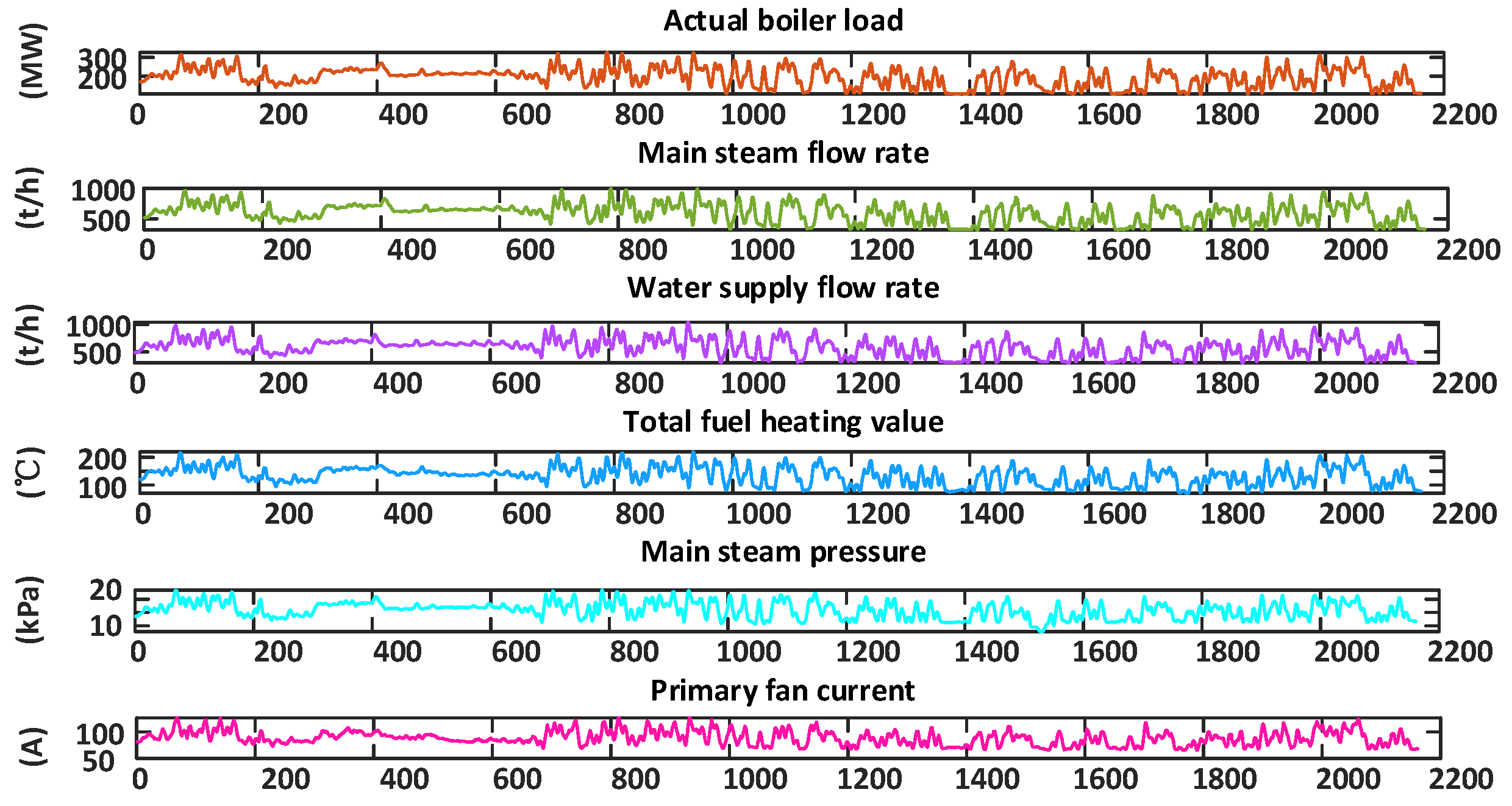
| No. | Input Variables | Maximum Value | Minimum Value | Unit |
|---|---|---|---|---|
| 1 | Actual boiler load | 353 | 101.12 | MW |
| 2 | Main steam temperature | 571.9 | 517.13 | °C |
| 3 | Main steam flow rate | 1079.76 | 307.08 | t/h |
| 4 | Main steam pressure | 24.75 | 7.64 | MPa |
| 5 | Outlet steam temperature of reheater | 568.39 | 491.15 | °C |
| 6 | Superheater outlet header’s outlet temperature | 574.66 | 498.43 | °C |
| 7 | Water temperature of boiler feed | 280 | 212.67 | °C |
| 8 | Water supply flow rate | 115.75 | 282.79 | t/h |
| 9 | Total fuel heating value | 245.27 | 67.4 | kJ/°C |
| 10 | Total primary air volume | 443.54 | 204.77 | t/h |
| 11 | Total secondary air volume | 810.76 | 247.44 | t/h |
| 12 | #1 Primary fan current | 142.43 | 65.57 | A |
| 13 | #2 Primary fan current | 169.95 | 67.23 | A |
| 14 | #1 Supply fan current | 46.6 | 0.14 | A |
| 15 | #2 Supply fan current | 49.91 | 15.8 | A |
| 16 | Flue gas temperature of low-temperature superheater | 589.62 | 412.85 | °C |
| 17 | Outlet flue gas pressure of low temperature reheater | −0.04 | −0.49 | kPa |
| 18 | Temperature of flue gas at the outlet of the economizer | 440.97 | 300.56 | °C |
| 19 | Flue gas temperature of air preheater outlet | 144.76 | 103.36 | °C |
| Input Variables | Correlation |
|---|---|
| Boiler feed | 0.8844 |
| Actual boiler load | 0.8352 |
| Main steam flow rate | 0.8347 |
| Total fuel heating value | 0.82 |
| Flow rate of the water supply | 0.8189 |
| Total primary air volume | 0.8011 |
| Main steam pressure | 0.7827 |
| Total secondary air volume | 0.7319 |
| #2 Primary fan current | 0.7273 |
| #1 Primary fan current | 0.6868 |
| Flue gas temperature at the air preheater outlet | 0.6457 |
| Temperature of flue gas at the outlet of the economizer | 0.6306 |
| Flue gas temperature of the low-temperature superheater | 0.6214 |
| Outlet steam temperature of reheater | 0.6098 |
| #1 Supply fan current | 0.4826 |
| #2 Supply fan current | 0.4786 |
| Main steam temperature | 0.3829 |
| Superheater outlet header’s outlet temperature | 0.1882 |
| Flue gas pressure at the low-temperature reheater outlet | 0.1453 |
| Parameter | Numerical Value |
|---|---|
| Delay time step | 5 |
| Population size | 10 |
| Learning rate | [0.001, 0.01] |
| Maximum iterations | 100 |
| Count of the hidden layers’ nodes | [16, 72] |
| Regularization parameter | () |
| Model | Learning Rate | Regularization Coefficient | Hidden Units |
|---|---|---|---|
| WOA-LSTM | 0.0083 | 43 | |
| PSO-LSTM | 0.0073 | 20 |
| Model | RMSE | MAE | MAPE | ||
|---|---|---|---|---|---|
| Training set | LSSVM | 0.19375 | 0.13189 | 0.25188% | 0.99979 |
| LSTM | 0.4494 | 0.34872 | 6.8337% | 0.92652 | |
| PSO-LSSVM | 0.04384 | 0.03164 | 0.58173% | 0.99891 | |
| PSO-LSTM | 0.17671 | 0.13837 | 2.6316% | 0.98231 | |
| WOA-LSTM | 0.14019 | 0.10789 | 2.0025% | 0.98864 | |
| Test set | LSSVM | 0.56778 | 0.39939 | 7.1514% | 0.84169 |
| LSTM | 0.45506 | 0.3729 | 6.255% | 0.89831 | |
| PSO-LSSVM | 0.27478 | 0.20416 | 3.5814% | 0.96292 | |
| PSO-LSTM | 0.19836 | 0.15445 | 2.7191% | 0.97068 | |
| WOA-LSTM | 0.16493 | 0.12712 | 2.2254% | 0.98664 |
Disclaimer/Publisher’s Note: The statements, opinions and data contained in all publications are solely those of the individual author(s) and contributor(s) and not of MDPI and/or the editor(s). MDPI and/or the editor(s) disclaim responsibility for any injury to people or property resulting from any ideas, methods, instructions or products referred to in the content. |
© 2024 by the authors. Licensee MDPI, Basel, Switzerland. This article is an open access article distributed under the terms and conditions of the Creative Commons Attribution (CC BY) license (https://creativecommons.org/licenses/by/4.0/).
Share and Cite
Wang, Y.; Li, Z.; Zhang, N. A Hybrid Soft Sensor Model for Measuring the Oxygen Content in Boiler Flue Gas. Sensors 2024, 24, 2340. https://doi.org/10.3390/s24072340
Wang Y, Li Z, Zhang N. A Hybrid Soft Sensor Model for Measuring the Oxygen Content in Boiler Flue Gas. Sensors. 2024; 24(7):2340. https://doi.org/10.3390/s24072340
Chicago/Turabian StyleWang, Yonggang, Zhida Li, and Nannan Zhang. 2024. "A Hybrid Soft Sensor Model for Measuring the Oxygen Content in Boiler Flue Gas" Sensors 24, no. 7: 2340. https://doi.org/10.3390/s24072340
APA StyleWang, Y., Li, Z., & Zhang, N. (2024). A Hybrid Soft Sensor Model for Measuring the Oxygen Content in Boiler Flue Gas. Sensors, 24(7), 2340. https://doi.org/10.3390/s24072340