1. Introduction
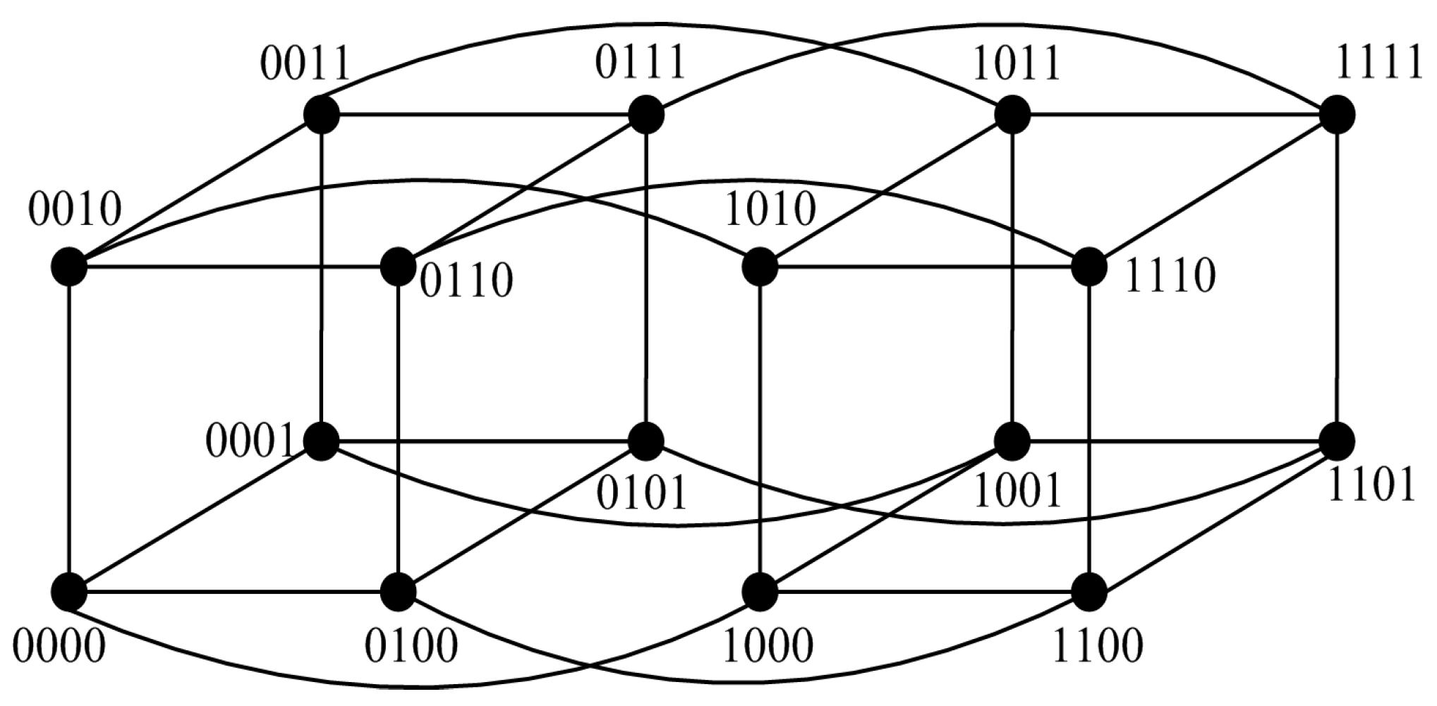
With the rapid advancement of information technology, the precision of very large-scale integration (VLSI) is becoming increasingly sophisticated. Today’s supercomputers may have thousands of processors. Take the US supercomputer Summit, which was crowned the world’s fastest super computer in 2018 and 2019, for example; it has 9216 processors. The large scale of its processor numbers may cause many unreliability problems. Therefore, reliability is an important issue to consider in the design, operation, and maintenance of such a large-scale multiprocessor system. To maintain system reliability, it is necessary to quickly identify all faults. The procedure of recognizing faults is known as fault diagnosis. System-level diagnosis is considered an ideal fault diagnostic method [
1].
Many important diagnostic strategies have been proposed in the course of the development of system-level fault diagnosis theory. Among them, the diagnostic capability of the original diagnostic strategy introduced by Preparata et al. [
1], named t-diagnosis, is relatively weak. To improve the diagnostic capability, another important diagnostic strategy, called
-diagnosis [
2], which requires all faulty nodes to be isolated in a set of nodes, was proposed by Somani et al. In this approach, at most
k nodes can be misdiagnosed if the fault node number does not exceed
t. For the system
G, its
-diagnosability is the maximum value of
t satisfying the condition that
G is
-diagnosable. For example, the hypercube is an important network topology, which has been applied to many parallel and distributed systems such as iWarp [
3] and Cray T3D [
4]. For
and
, it is proved by Somani et al. [
2] that the hypercube
is
-diagnosable. The
-diagnosability of several networks under the PMC model has been determined, including hypercubes [
2], star graphs [
2,
5], mesh-based systems [
2], and bijective connection (BC) networks [
6,
7]. Recently, by utilizing the properties of the 0-test subgraph under the PMC model, Lin et al. [
8] studied the
-diagnosability of regular graphs under the PMC model.
It is well known that there are three system-level diagnosis models: the BGM model [
9], the comparison model [
10], and the PMC model. The BGM model is not often used in the existing literature as a fault diagnosis model due to its flaws. It is worth mentioning as Sengupta and Dahbura state[
10], the comparison diagnosis model can be obtained by generalizing the PMC model. In other words, in terms of diagnosis model, the comparison model is often more suitable than the PMC model for studying the system fault diagnosis. However, to the best of our knowledge, to date, few studies have investigated
-diagnosability under the comparison model. In this paper, we study the problem of
-diagnosability for regular networks under the comparison model.
The main contributions of this paper are described below.
To study -diagnosability based on the comparison model, the paper introduces some important definitions, such as the 0-test unit and 0-test subgraph, and present their related properties;
We present the description of the -diagnosability of regular networks under the comparison model. At the same time, we propose a -diagnosis algorithm for regular networks under the comparison model, which is, to the best of our knowledge, the first such -diagnosis algorithm for regular networks under the comparison model;
We give the -diagnosabilities for some famous network systems such as hypercube networks, star networks, complete cubic networks, and so on.
The rest of the paper is organized as follows. In the following section, some necessary terminologies and notations are presented. We introduce the definition and properties of the 0-test subgraph in
Section 3.
Section 4 presents the main results of this paper. We discuss some applications in
Section 5.
Section 6 concludes the paper.
2. Preliminaries
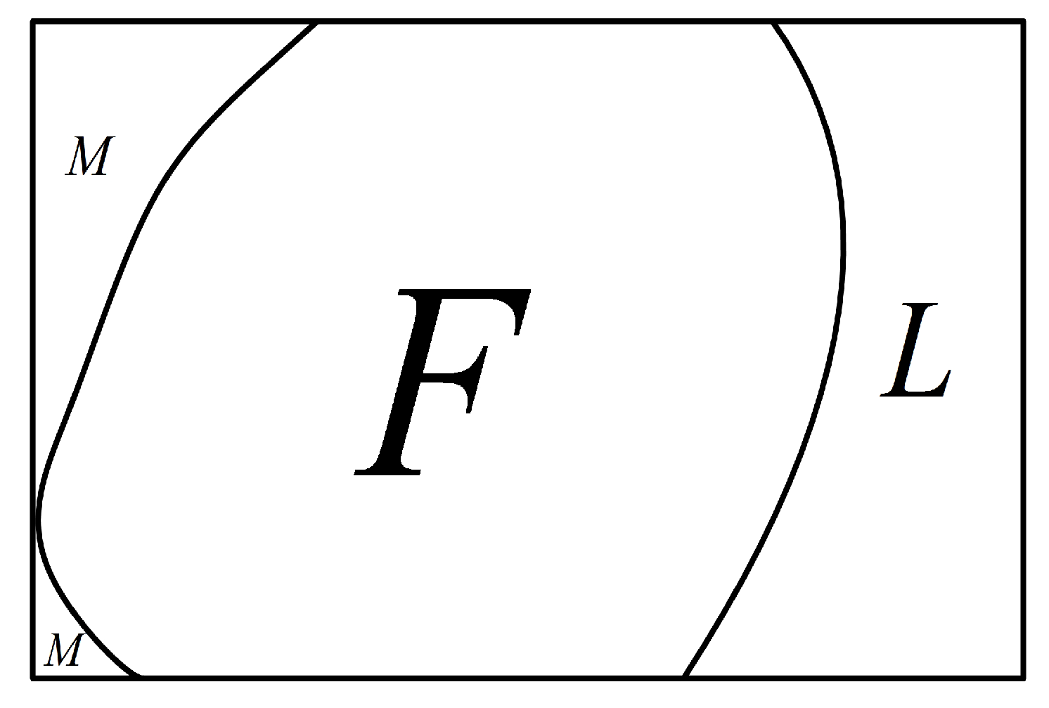
A multiprocessor system can be modeled as a graph , with being the node set and being the edge set. For , is the set of all the neighbors of x, and is the degree of x in G. Let and . Then, and , where and .
In a connected graph, nodes with degree 1 are known as pendant nodes. A pendant edge is incident to at least one pendant node. Then, all the nodes and edges in
G can be classified into two types: pendant and non-pendant. Let
and
be the sets of pendant nodes and non-pendant nodes, and let
and
be the sets of pendant edges and non-pendant edges, respectively, (see
Figure 1). Then, we have the following properties.
Lemma 1. If G is a connected graph with , then .
Proof of Lemma 1. Since
G is connected with
, there exist no edges whose two endpoints are pendant nodes. That is, each pendant edge corresponds to a different pendant node (see
Figure 1). Therefore,
. □
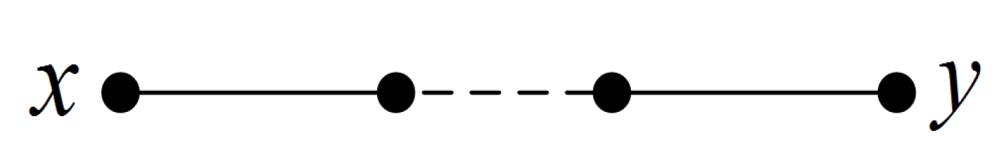
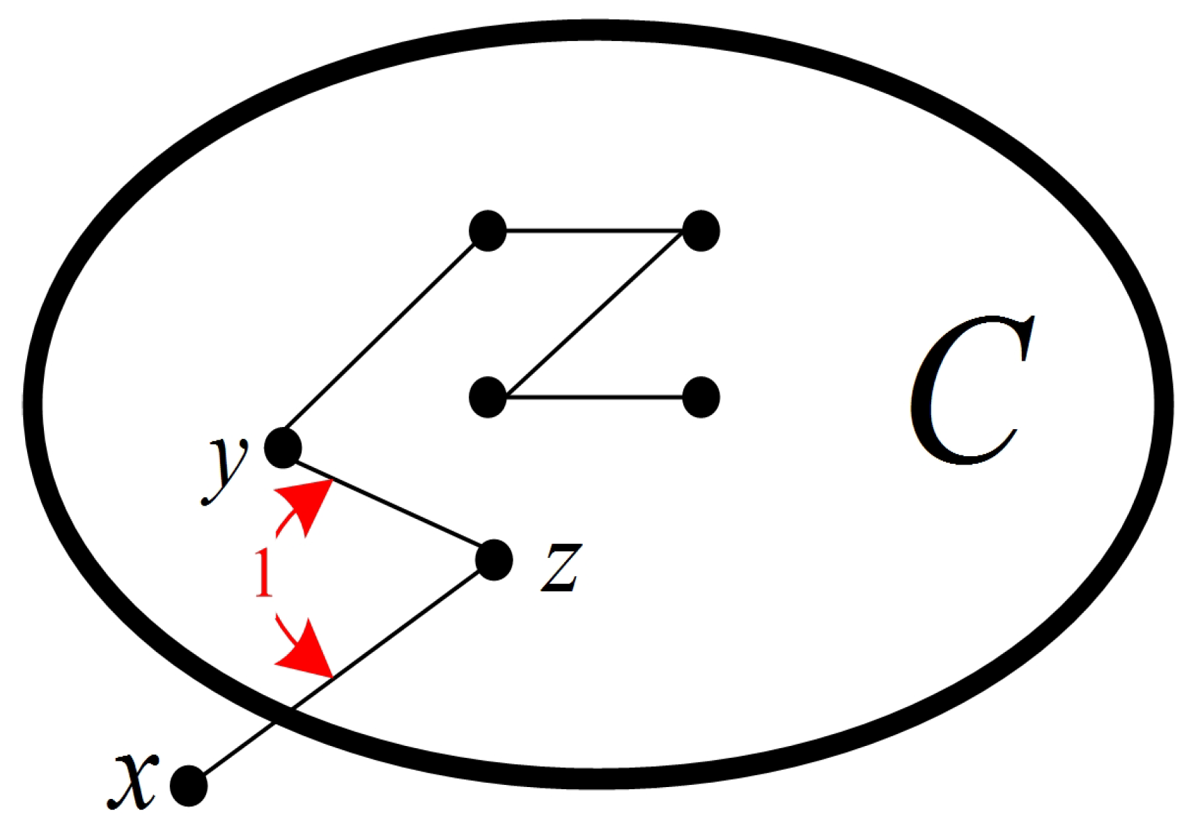
Lemma 2. is connected.
Proof of Lemma 2. For any two nodes
, since
G is connected, there exists a path that connects
x and
y (see
Figure 2). Since each node in
has degree 1, the path will not pass through any node in
. Thus, there is a path that connects
x and
y in
. Therefore,
is connected. □
Lemma 3. Let be a connected graph satisfying and . Then, .
Proof of Lemma 3. We have
. By Lemma 2,
is connected. That is, all nodes in
are connected by edges in
. Clearly,
. Assume the average degree in
is
a with
. By Lemma 1,
. According to Euler’s handshaking lemma, we have
Therefore,
. □
In system-level diagnosis, the PMC model [
1] and comparison model [
10] are two widely adopted diagnostic models. Under the comparison model, a comparator will distribute a task to its two adjacent nodes and compare the responses they provide. The comparison of nodes
x and
y performed by
z is denoted by
, where
and
denote two test edges, respectively. The outcome of test
is represented by
. In
Table 1, the invalidation rules for the comparison model are summarized. By
Table 1, if
, all three nodes are fault-free or the tester
z is faulty. Moreover, if
x and
z are fault-free, we can identify
y as fault-free by
or as faulty by
.
A collection of all the test results is called a syndrome . For a given syndrome , F is called an allowable faulty set if can be produced from F, i.e., if the following two conditions hold:
- (a)
for ;
- (b)
for and (or ).
For a given syndrome , if there are several allowable faulty sets , we cannot accurately diagnose the set. As a result, the faulty nodes can only be isolated into a set F, such that .
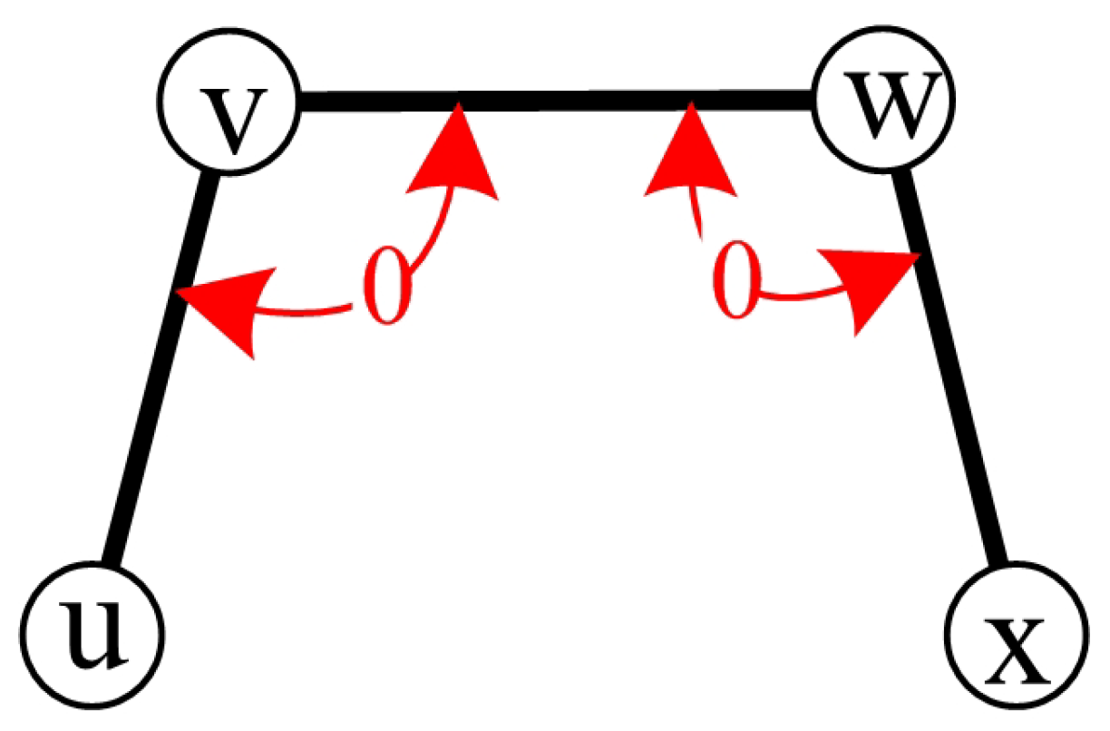
3. 0-Test Subgraph under the Comparison Model
For a given a syndrome
under the comparison model, test
is a 0-test unit if
, where
and
are two test edges. The two tests,
and
, belong to the same 0-test set because they share at least one common test edge (see
Figure 3). The graph induced by a 0-test set is called a 0-test subgraph.
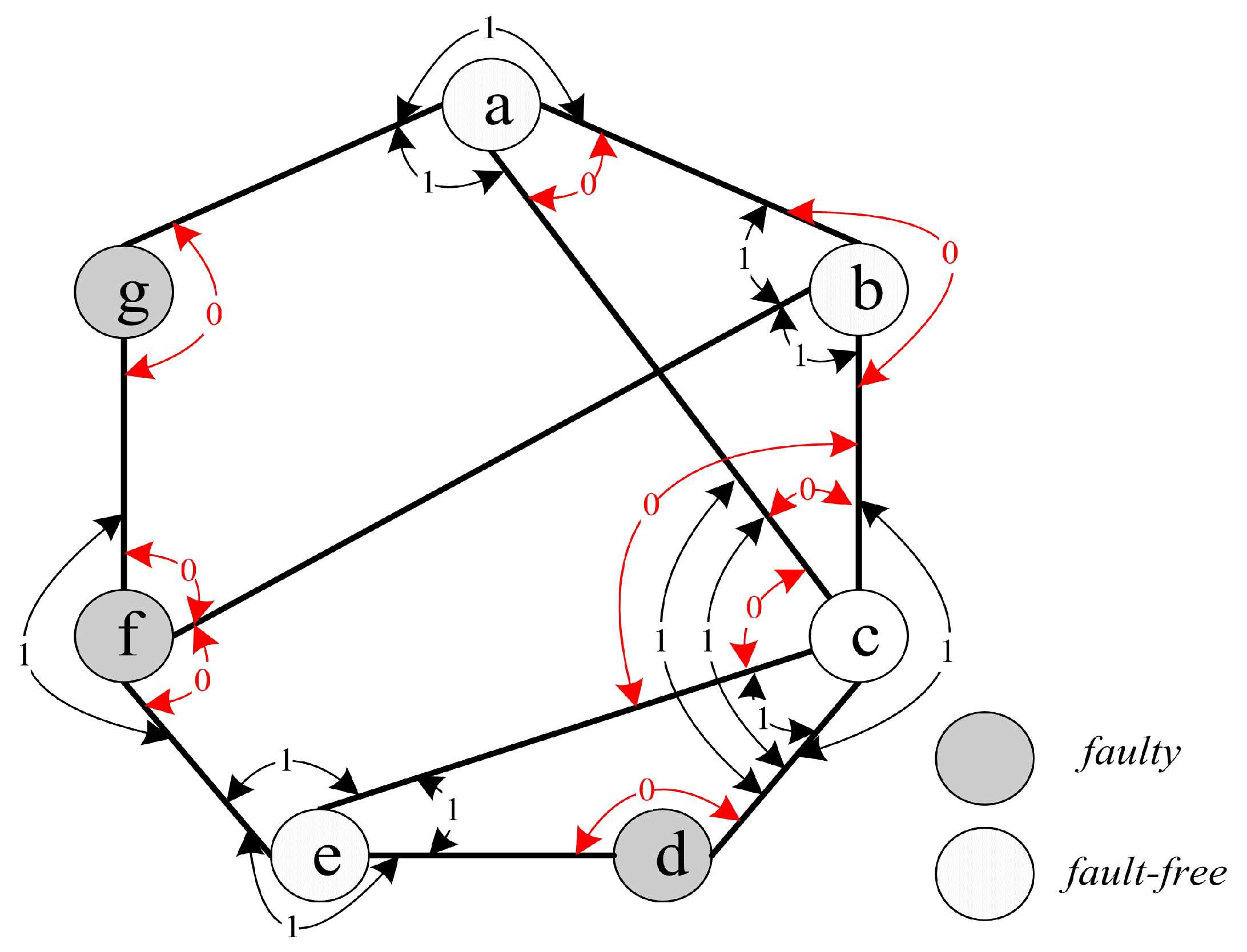
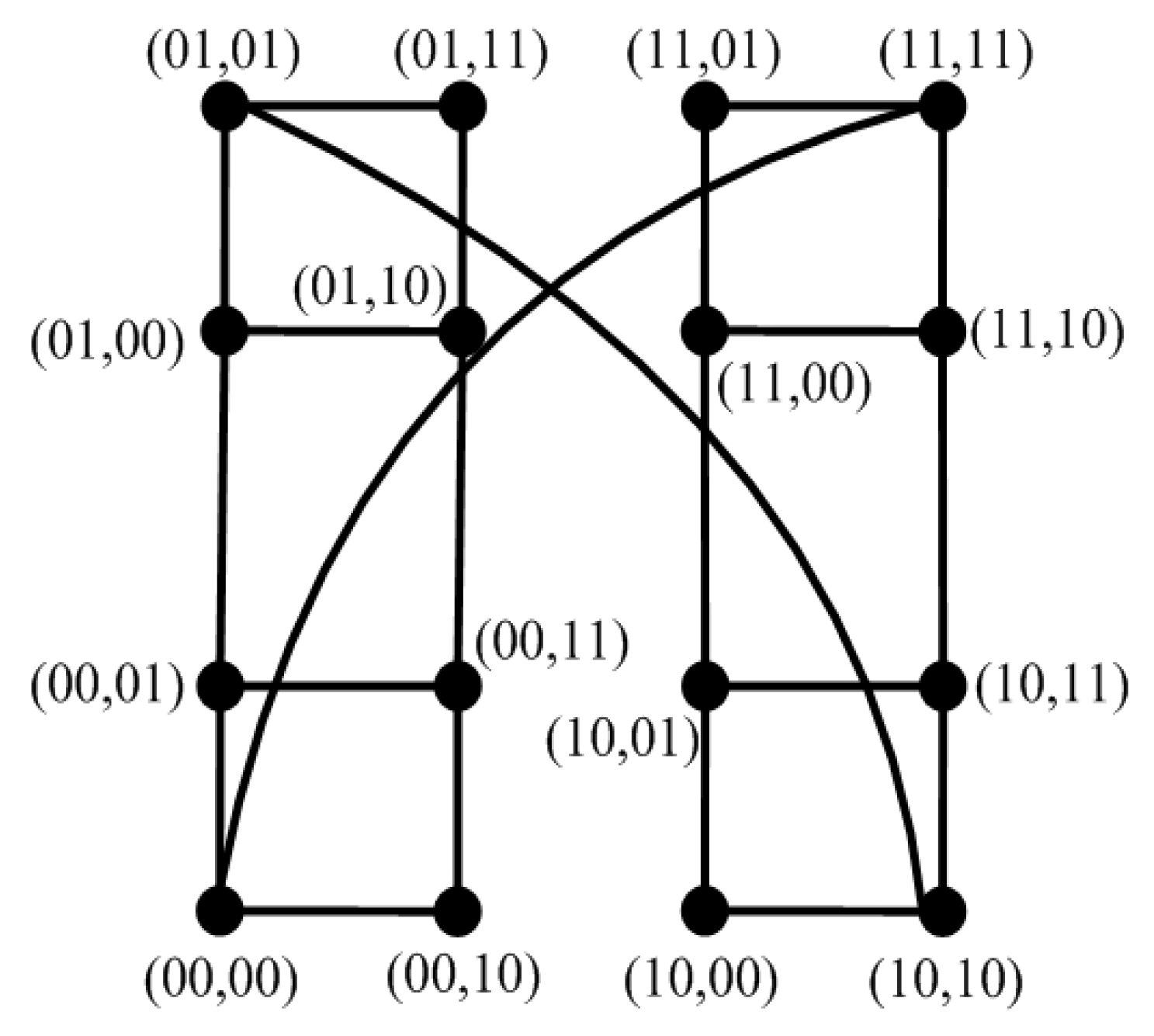
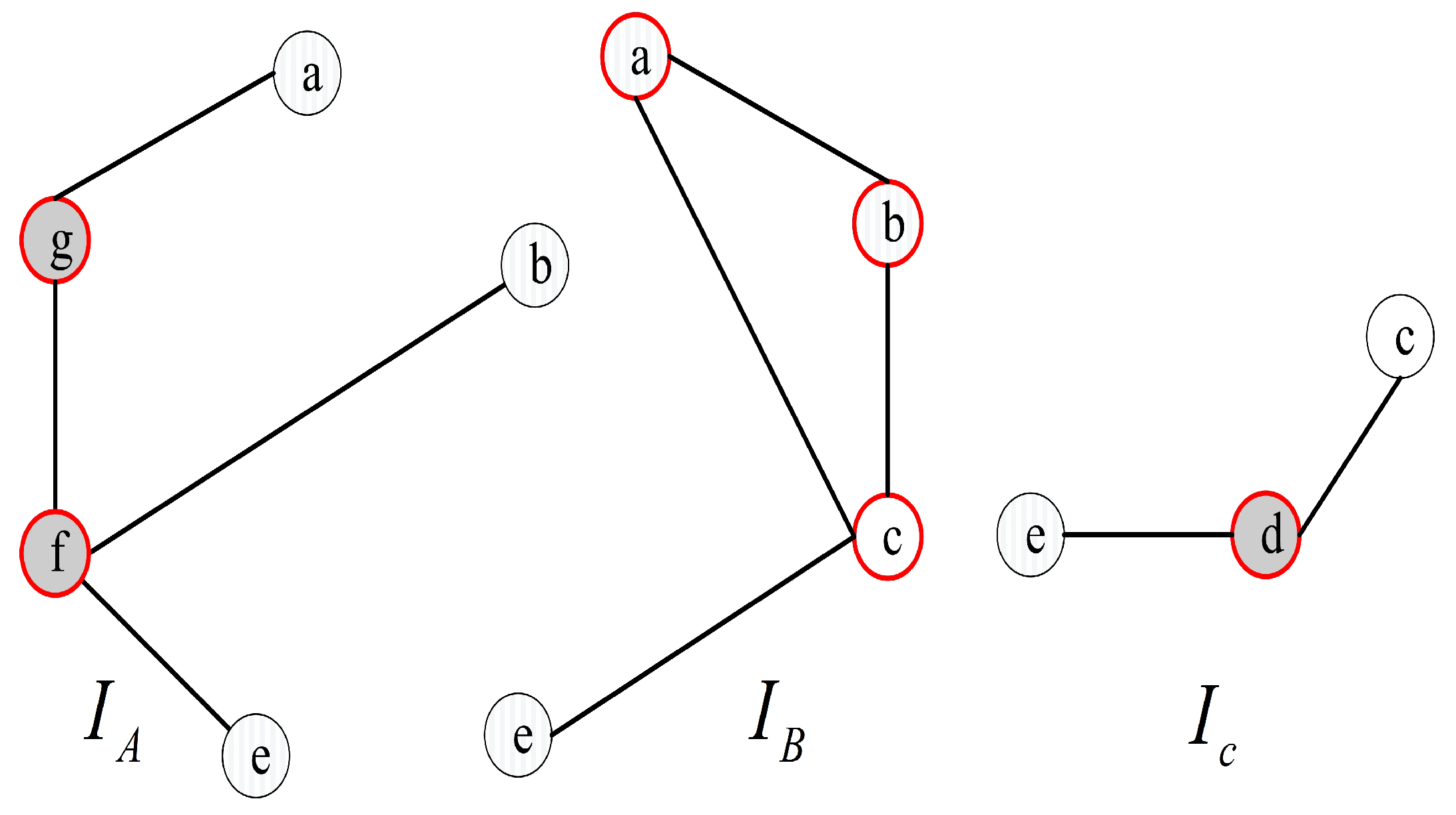
For instance, we have
(see
Figure 4). The syndrome under the comparison model is represented in
Figure 4, where
,
,
,
,
,
,
,
, and
, and the outcomes of other tests are 1. Hence, there are nine 0-test units,
,
,
,
,
,
,
,
, and
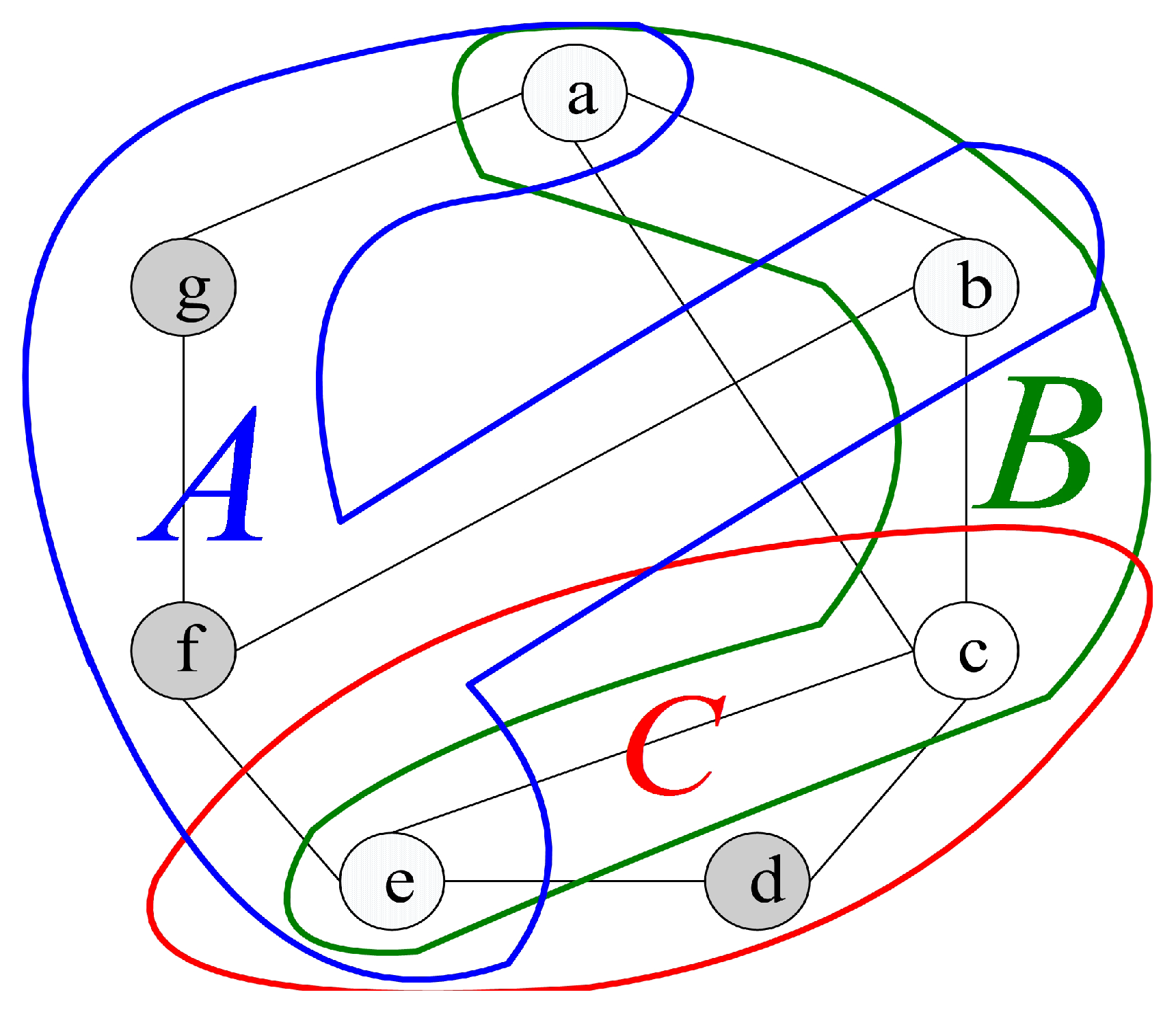
. Furthermore, there are three 0-test sets,
A={
,
,
},
B={
,
,
,
,
}, and
C={
} (see
Figure 5). Then, let
,
, and
be the 0-test subgraphs induced by 0-test sets
A,
B, and
C, respectively, (see
Figure 6). The set of all 0-test subgraphs of
G is written as
. For any
,
.
Let H be a 0-test set under the comparison model. Let represent the set consisting all testers in H. Clearly, all the testers in H are connected in H or . In the previous example, we have , , and . Then, we have the following properties.
Lemma 4. Let H be a 0-test set of G under the comparison model. Either all the nodes in H are fault-free or each node in is faulty.
Proof of Lemma 4. For arbitrary
,
. By
Table 1, all the nodes of
a,
b, and
c are fault-free or tester
a is faulty. Let
be another 0-test unit in
H that has a common test edge with
. We have
. If
a,
b, and
c are fault-free,
e is also fault-free because
. This process continues until all 0-test units in
H have been examined. Therefore, all the nodes in
H are fault-free. Otherwise,
a is faulty, since
,
c is also faulty by
Table 1. As a result, all the nodes in
are faulty. □
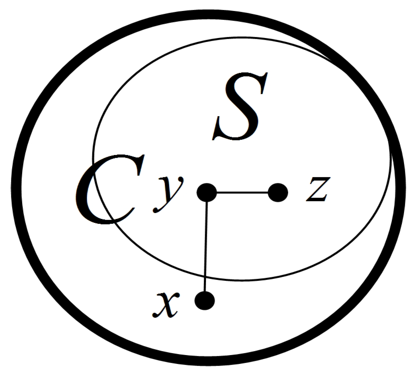
Lemma 5. Assume that F represents a fault set of G. For any component C of , C is a 0-test subgraph under the comparison model.
Proof of Lemma 5. Since
C is a component of
,
C is connected, and all the nodes in
C are fault-free with
. Hence, under the comparison model, any test in
C is a 0-test unit. Therefore,
C belongs to a 0-test subgraph
. For any
, without loss of generality, suppose that
with
(see
Figure 7). Then, we have
. Hence,
. That is, each node in
does not belong to
S. Therefore,
. □
Lemma 6. Let S represent a 0-test subgrapht corresponding a component C of under the comparison model. Then, .
Proof of Lemma 6. Since C is connected and all the nodes in C are fault-free, we have . For an arbitrary 0-test unit in S, tester a has at least two neighbors x and y in C. Thus, . Then, we have . Therefore, . □
Lemma 7. Let F be a fault set of G and let with ; then, S is a component of .
Proof of Lemma 7. Since
, by Lemma 4, all the nodes in
S are fault-free. Moreover, since
S is a connected subgraph,
S belongs to component
C of
, denoted by
. Suppose that
. Since
C is connected,
satisfying
(see
Figure 8). We let
such that
. Since
,
. There exists another node
with
. Furthermore, since
C is a component of
,
. Thus,
. By the definition of the 0-test subgraph,
, which contradicts
. Therefore,
. □
4. -Diagnosability and a -Diagnosis Algorithm under the Comparison Model
In the section, we discuss the -diagnosability for a given regular network . The outline of the section is as follows. First, we prove that for a fault set S with and , contains a large component H with and the number of nodes in is no more than nodes. Next, we discuss the sufficient conditions for the result that G is -diagnosable under the comparison model. Finally, based on the obtained sufficient conditions and depth-first search strategy, we design a -diagnosis algorithm for computing a fault set F with for the regular network G such that at most k free-fault nodes belong to F.
Suppose that is a function of integer k with and ; the following three conditions are used in the rest of this paper.
Condition 1. For any with , contains a large component H such that and ;
Condition 2. ;
Condition 3. .
Then, we can derive some theorems and corollaries as follows.
Corollary 1. Let S be a fault set of G with and . If Conditions 1 and 3 hold, has a large component H with , and the union of the remaining components M has a maximum nodes.
Proof of Corollary 1. Let F be a set with . By Condition 1, contains a large component L such that and .
By Condition 3, . According to the conclusion of the previous paragraph, for any with , has a large component H such that and . □
Theorem 1. Let F be a fault set of G with . If Condition 2 holds and contains a large component L with , then with .
Proof of Theorem 1. By Condition 2 and
, we can obtain
Therefore, we have
, for
.
Since and L is a connected component, . By Lemma 3, we have . By Lemma 5, L is a 0-test subgraph under the comparison model, denoted by . Moreover, by Lemma 6, we have . □
Theorem 2. If Conditions 1 and 2 hold, G is -diagnosable under the comparison model.
Proof of Theorem 2. Let F be a fault set of G with . According to Condition 1, contains a large component L with . By Theorem 1, with . That is, there exists a 0-test subgraph L such that and . By Lemma 7, all the nodes in L can be identified as fault-free. Since , there are fewer than nodes that are unidentified. Hence, all the faulty nodes can be isolated into a node set, in which the number of fault-free nodes is no more than k. Therefore, under the comparison model, G is -diagnosable. □
Furthermore, we continue to search for a higher value of t such that the system is -diagnosable.
Theorem 3. If Conditions 1–3 hold, then, under the comparison model, G is -diagnosable.
Proof of Theorem 3. Let F be a fault set of G with . Now, we discuss the situation by considering the following scenarios.
Case 1.
According to Condition 1, contains a large component H with and . By Theorem 1, with . Moreover, by Lemma 7, all the nodes in H can be identified as fault-free. Since , there are fewer than unidentified nodes. Therefore, all the faulty nodes can be isolated in a node set containing a maximum bound of k fault-free nodes.
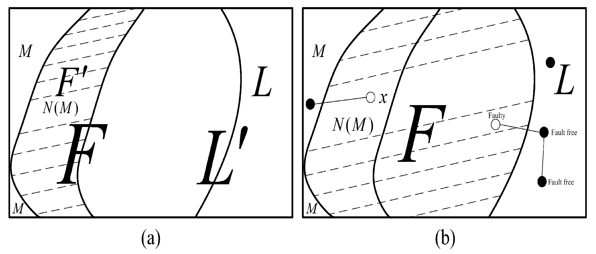
Case 2.
By Corollary 1,
has a large component
L with
, and the union of the remaining components
M has a maximum of
nodes (see
Figure 9). We have
. By Theorem 1,
L is a 0-test subgraph with
. Hence, by Lemma 7, all the nodes in
L can be identified as fault-free. There is a total of
nodes that remain unidentified.
Case 2.1. .
Since , all faulty nodes can be isolated within a node set that at most k fault-free nodes are contained.
Case 2.2. .
Suppose that
. Let
; we have
. By Condition 1,
has a large component
and a union of remaining components
with
(see
Figure 10a). Since
and
,
. Therefore,
and
. Then,
, which contradicts
. Therefore,
. Since
and
, we have
and
. That is, each node in
F has a neighbor in
M.
Suppose that
and
(see
Figure 10b). Let
; we have
. According to Condition 1,
has a union of smaller components
with
and a large component. Then,
. Therefore,
, which contradicts
. Hence, each node in
F is connected to at least one neighbor in
L. That is,
.
Since all the nodes belonging to
L are fault-free, all the nodes in
F can be identified as faulty (see
Figure 10b), where
. Note that
, all nodes in
M are identified as fault-free. Thus, all faulty nodes can be isolated within a node set, and no fault-free node is misidentified as faulty. Therefore, under the comparison model,
G is
-diagnosable. □
Inspired by Lin et al. [
8], we introduce a
t/
k-diagnosis Algorithm 1 under the comparison model.
| Algorithm 1: t/k-diagnosis algorithm under the comparison model |
Require: Conditions 1–3. Ensure: , where H is the set of nodes that are identified as fault-free and is the set of nodes that are isolated. Step 1. , ; Step 2. Use a depth-first traversal algorithm to derive all the 0-test units under the comparison model; Step 3. Obtain the tester of each 0-test units and merge 0-test units to construct , and set ; Step 4. Compute for , by merging testers in ; Step 5. For each 0-test subgraph , if , then ; Step 6. ; Step 7. If , then ; else, ; Step 8. Return . |
The correctness of the
-diagnosis algorithm under the comparison model follows from Theorem 3. In this algorithm, steps 1 and 4–8 take
time. In step 2, the main computational process is based on pairs of adjacent edges. There are
pairs of adjacent edges. Step 3 is based on 0-test units. In the worst case, step 3 need
iterations to compare each pair of 0-test units to see if they have a common test edge. Take an
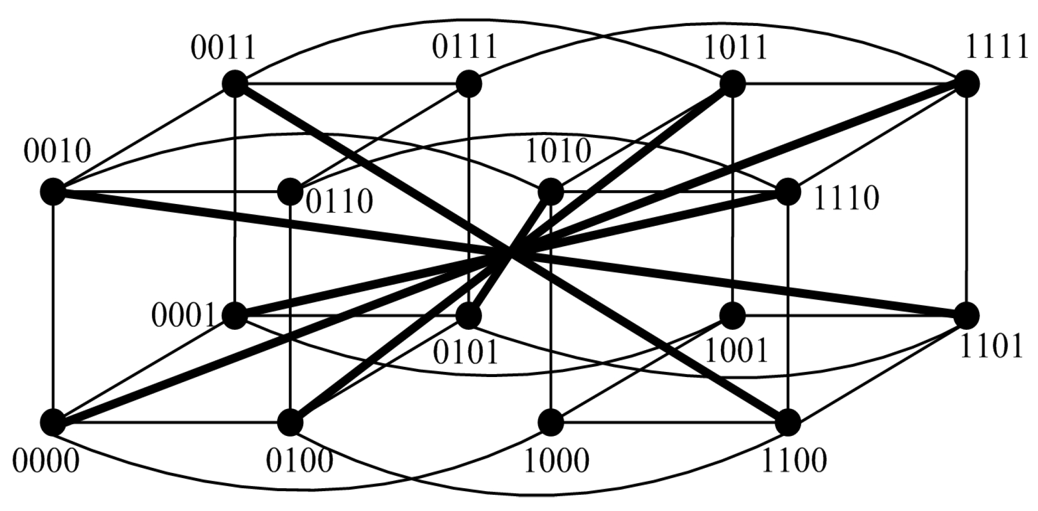
n-dimensional hypercube network
as an example,
is an
n-regular graph with
[
11]. Let
, we have
. Then,
. Hence, steps 2 and 3 take
time. As a result, the total time needed by this algorithm for n-dimensional hypercube networks is
, where
.
6. Conclusions
-diagnosability is an important diagnostic strategy that can improve the self-diagnosing capability of multiprocessor systems. While significant progress has been made in -diagnosability under the PMC model in the last half century, -diagnosability and -diagnosis algorithms for many regular networks under the comparison model have yet to be determined. In this paper, inspired by the 0-test subgraph under the PMC model, we introduce some useful notions for the comparison model, such as the 0-test unit, 0-test set, and 0-test subgraph. Then, we study the properties of 0-test subgraphs under the comparison model. Furthermore, we derive some key theorems about -diagnosability and the -diagnosis algorithm under the comparison model. Finally, the applications of our results to some regular networks are demonstrated.
In the article, we calculate the -diagnosability for regular networks based on the comparison model. Considering that N-ary M-cube networks are more general than regular networks in terms of network topology, in the future, we will investigate the -diagnosability problem of N-ary M-cube networks under the comparison model.


