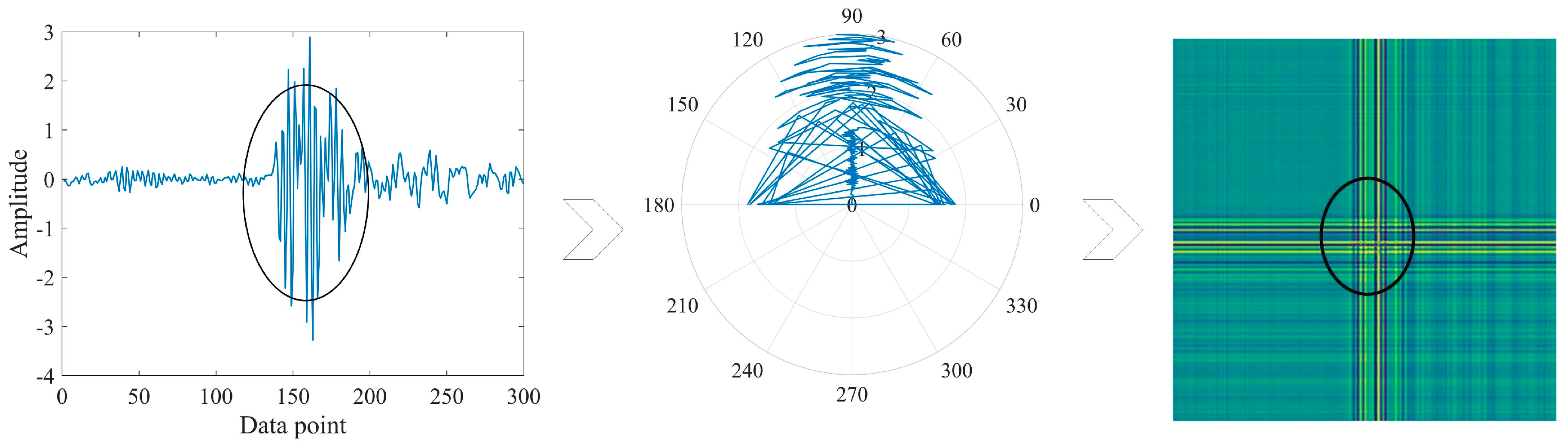
Figure 1.
GADF coding process.
Figure 1.
GADF coding process.
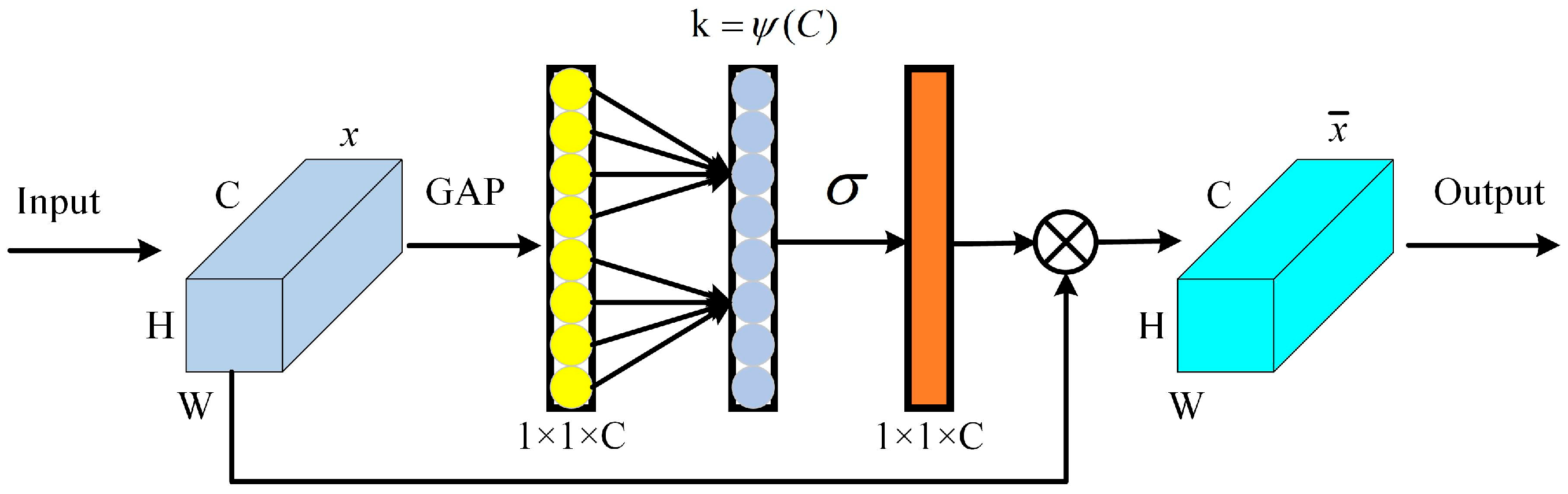
Figure 2.
Residual structure.
Figure 2.
Residual structure.
Figure 3.
Efficient Channel Attention (ECA).
Figure 3.
Efficient Channel Attention (ECA).
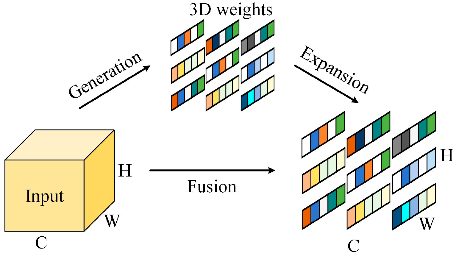
Figure 4.
SimAM structure.
Figure 4.
SimAM structure.
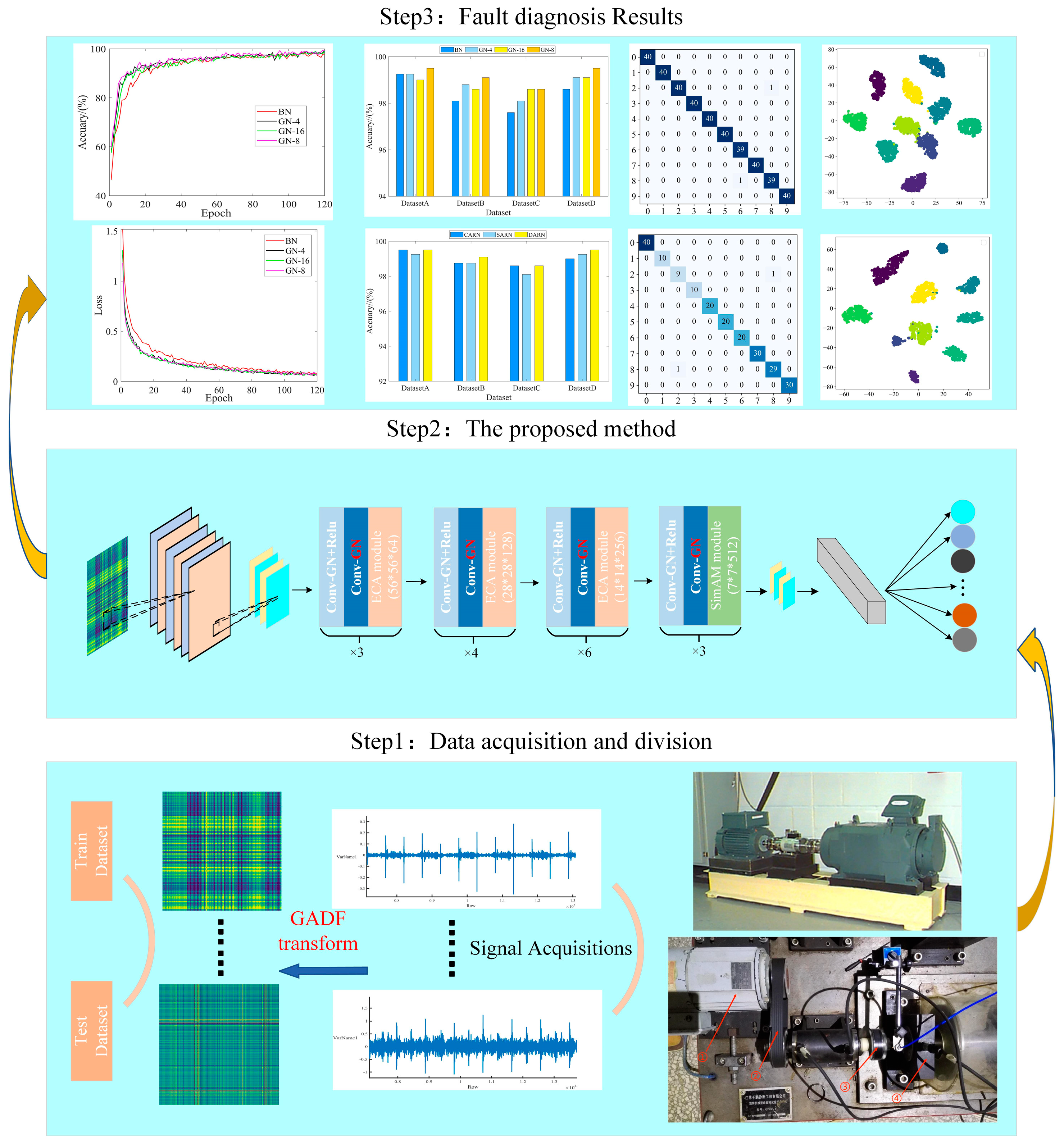
Figure 5.
IDARN model structure.
Figure 5.
IDARN model structure.
Figure 6.
Fault diagnosis process.
Figure 6.
Fault diagnosis process.
Figure 7.
Experimental equipment of CWRU [
24].
Figure 7.
Experimental equipment of CWRU [
24].
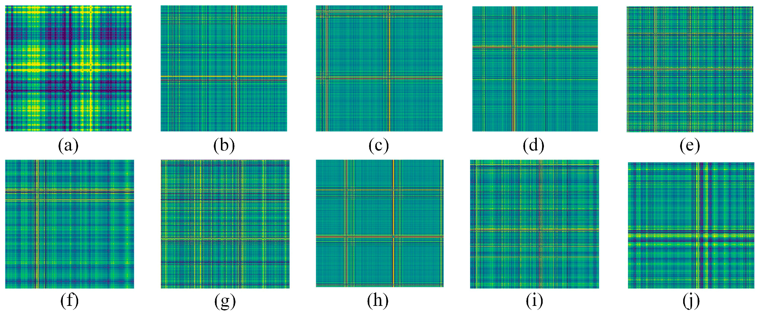
Figure 8.
Fault coded images. (a) NO; (b) IF-0.007in; (c) IF-0.014in; (d) IF-0.021in; (e) RE-0.007in; (f) RE-0.014in; (g) RE-0.021in; (h) OF-0.007in; (i) OF-0.014in; (j) OF-0.021in.
Figure 8.
Fault coded images. (a) NO; (b) IF-0.007in; (c) IF-0.014in; (d) IF-0.021in; (e) RE-0.007in; (f) RE-0.014in; (g) RE-0.021in; (h) OF-0.007in; (i) OF-0.014in; (j) OF-0.021in.
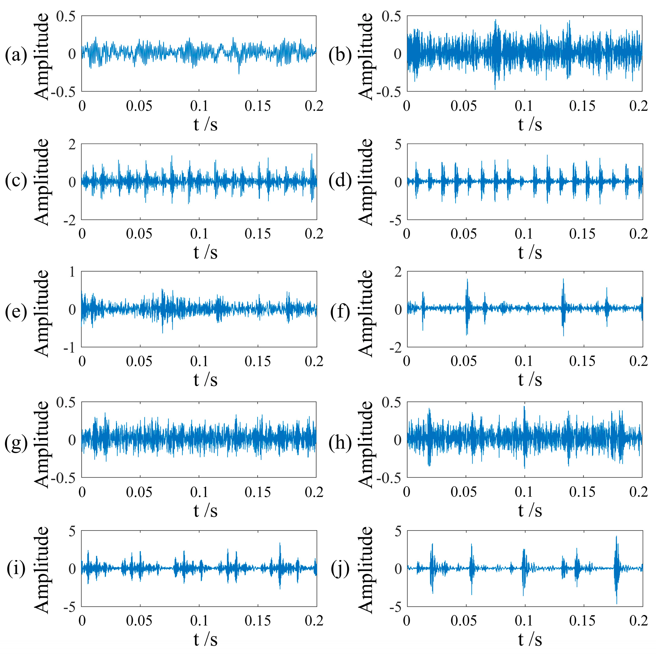
Figure 9.
Vibration images of faults. (a) NO; (b) RE-0.007in; (c) IF-0.007in; (d) OR-0.007in; (e) RE-0.014in; (f) IR-0.014in; (g) OF-0.014in; (h) RE-0.021in; (i) IF-0.021in; (j) OF-0.021in.
Figure 9.
Vibration images of faults. (a) NO; (b) RE-0.007in; (c) IF-0.007in; (d) OR-0.007in; (e) RE-0.014in; (f) IR-0.014in; (g) OF-0.014in; (h) RE-0.021in; (i) IF-0.021in; (j) OF-0.021in.
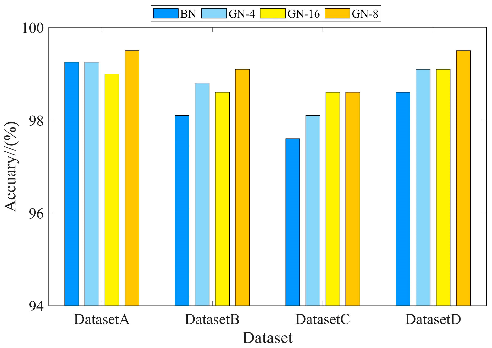
Figure 10.
Comparison of different normalisation methods.
Figure 10.
Comparison of different normalisation methods.
Figure 11.
Training performance curves of BN and GN method comparison. (a) Accuracy (DatasetA); (b) Loss (DatasetA).
Figure 11.
Training performance curves of BN and GN method comparison. (a) Accuracy (DatasetA); (b) Loss (DatasetA).
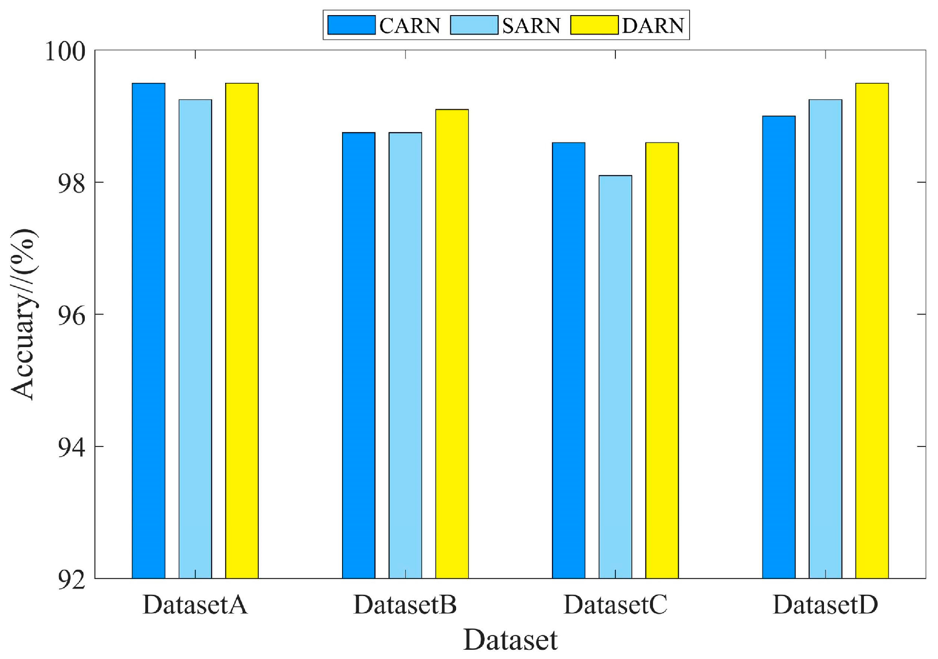
Figure 12.
Comparison of different methods of attention.
Figure 12.
Comparison of different methods of attention.
Figure 13.
Training performance curves. (a) Accuracy/DatasetA; (b) Loss/DatasetA; (c) Accuracy/DatasetB; (d) Loss/DatasetB.
Figure 13.
Training performance curves. (a) Accuracy/DatasetA; (b) Loss/DatasetA; (c) Accuracy/DatasetB; (d) Loss/DatasetB.
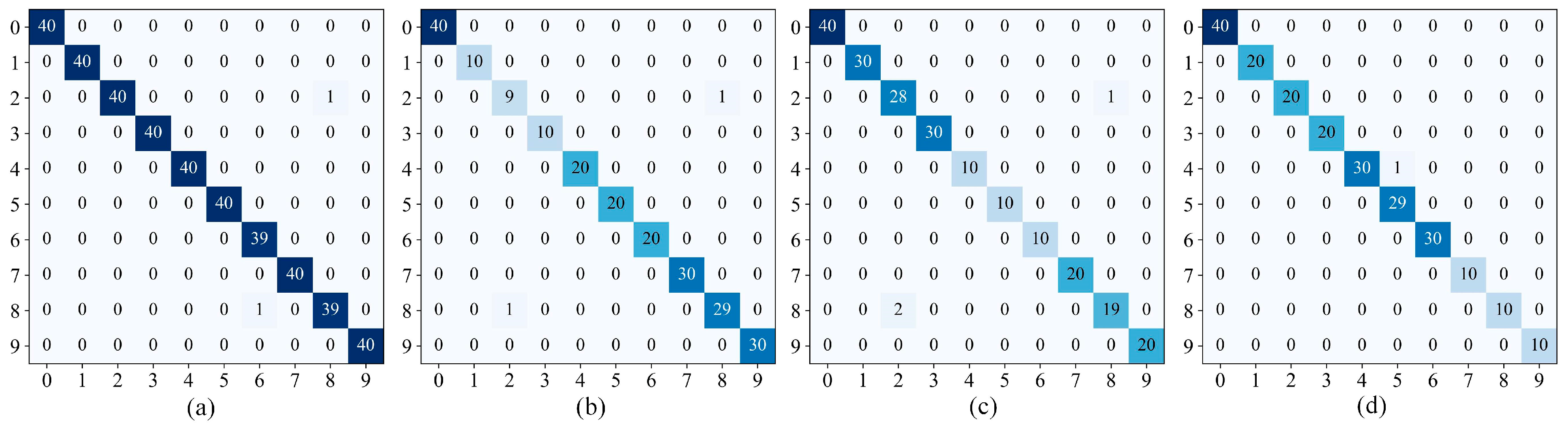
Figure 14.
Confusion matrices. (a) DatasetA; (b) DatasetB; (c) DatasetC; (d) DatasetD.
Figure 14.
Confusion matrices. (a) DatasetA; (b) DatasetB; (c) DatasetC; (d) DatasetD.
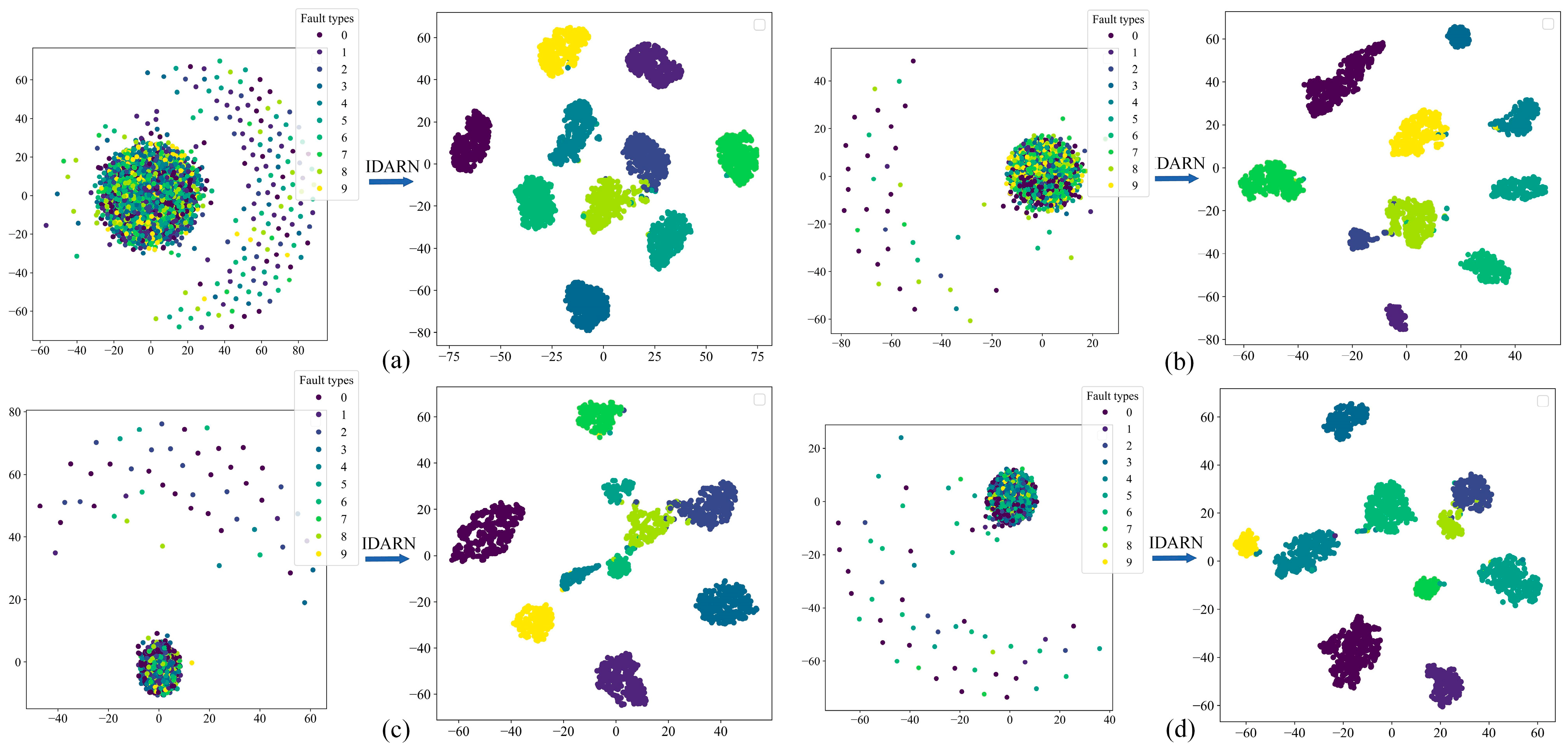
Figure 15.
t-SNE. (a) DatasetA; (b) DatasetB; (c) DatasetC; (d) DatasetD.
Figure 15.
t-SNE. (a) DatasetA; (b) DatasetB; (c) DatasetC; (d) DatasetD.
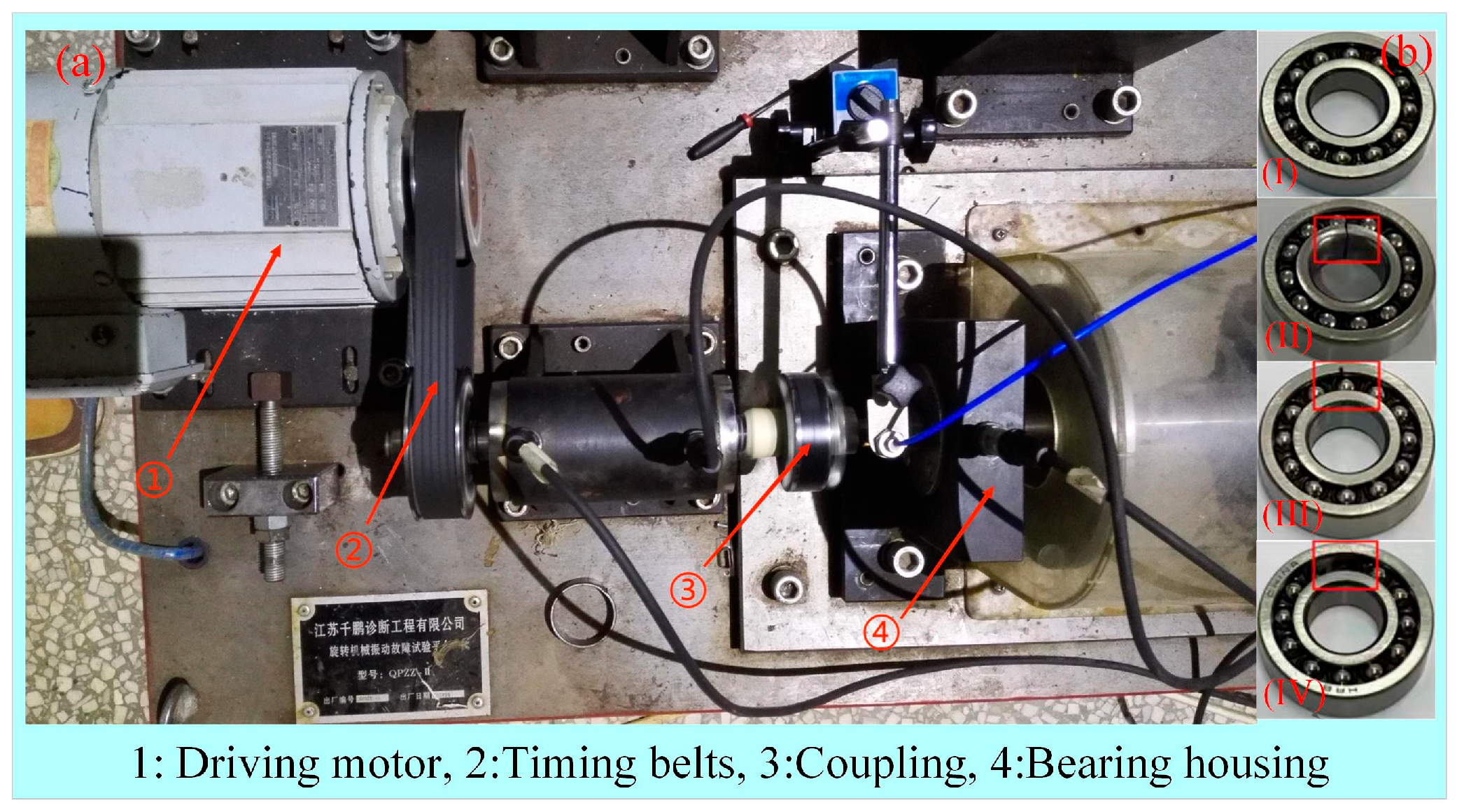
Figure 16.
Bearing fault experimental equipment. (a) Experimental equipment (QPZZ-II); (b) Different states of the bearings: (I) Normal; (II) Failure of the inner ring; (III) Failure of the outer ring; (IV) Roller body failure.
Figure 16.
Bearing fault experimental equipment. (a) Experimental equipment (QPZZ-II); (b) Different states of the bearings: (I) Normal; (II) Failure of the inner ring; (III) Failure of the outer ring; (IV) Roller body failure.
Figure 17.
Fault coded images. (a) NO; (b) IF-500; (c) IF-1000; (d) IF-1500; (e) OF-500; (f) OF-1000; (g) OF-1500; (h) RE-500; (i) RE-1000; (j) RE-1500.
Figure 17.
Fault coded images. (a) NO; (b) IF-500; (c) IF-1000; (d) IF-1500; (e) OF-500; (f) OF-1000; (g) OF-1500; (h) RE-500; (i) RE-1000; (j) RE-1500.
Figure 18.
Comparison results. (a) Dataset1; (b) Dataset2; (c) Dataset3.
Figure 18.
Comparison results. (a) Dataset1; (b) Dataset2; (c) Dataset3.
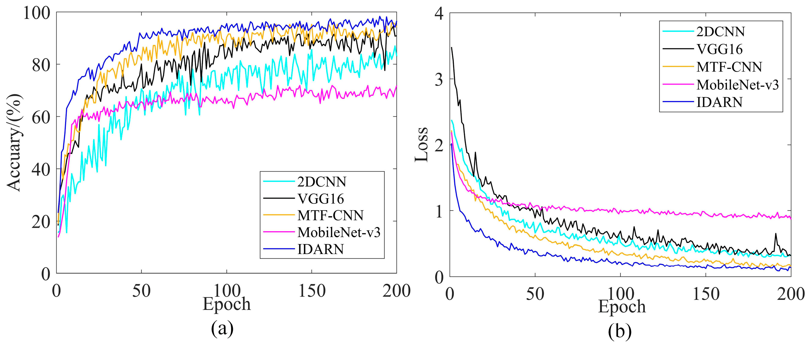
Figure 19.
Training performance curves for popular model comparisons. (a) Accuracy (Dataset1); (b) Loss (Dataset1).
Figure 19.
Training performance curves for popular model comparisons. (a) Accuracy (Dataset1); (b) Loss (Dataset1).
Figure 20.
Training performance curves for related model comparison. (a) Accuracy (Dataset2); (b) Loss (Dataset2).
Figure 20.
Training performance curves for related model comparison. (a) Accuracy (Dataset2); (b) Loss (Dataset2).
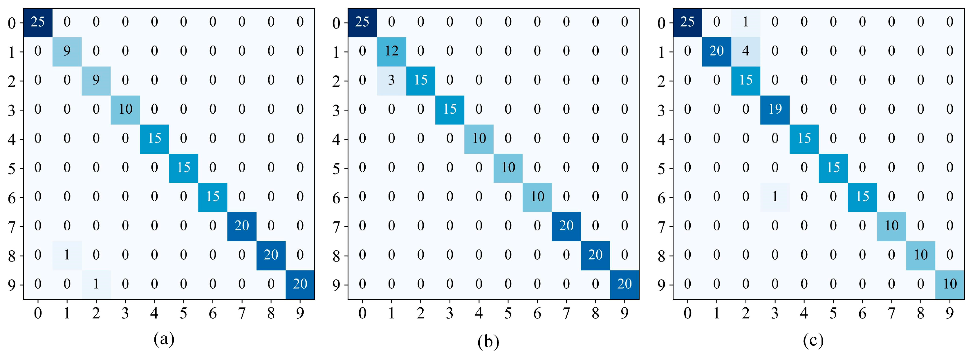
Figure 21.
Confusion matrices. (a) Dataset1; (b) Dataset2; (c) Dataset3.
Figure 21.
Confusion matrices. (a) Dataset1; (b) Dataset2; (c) Dataset3.
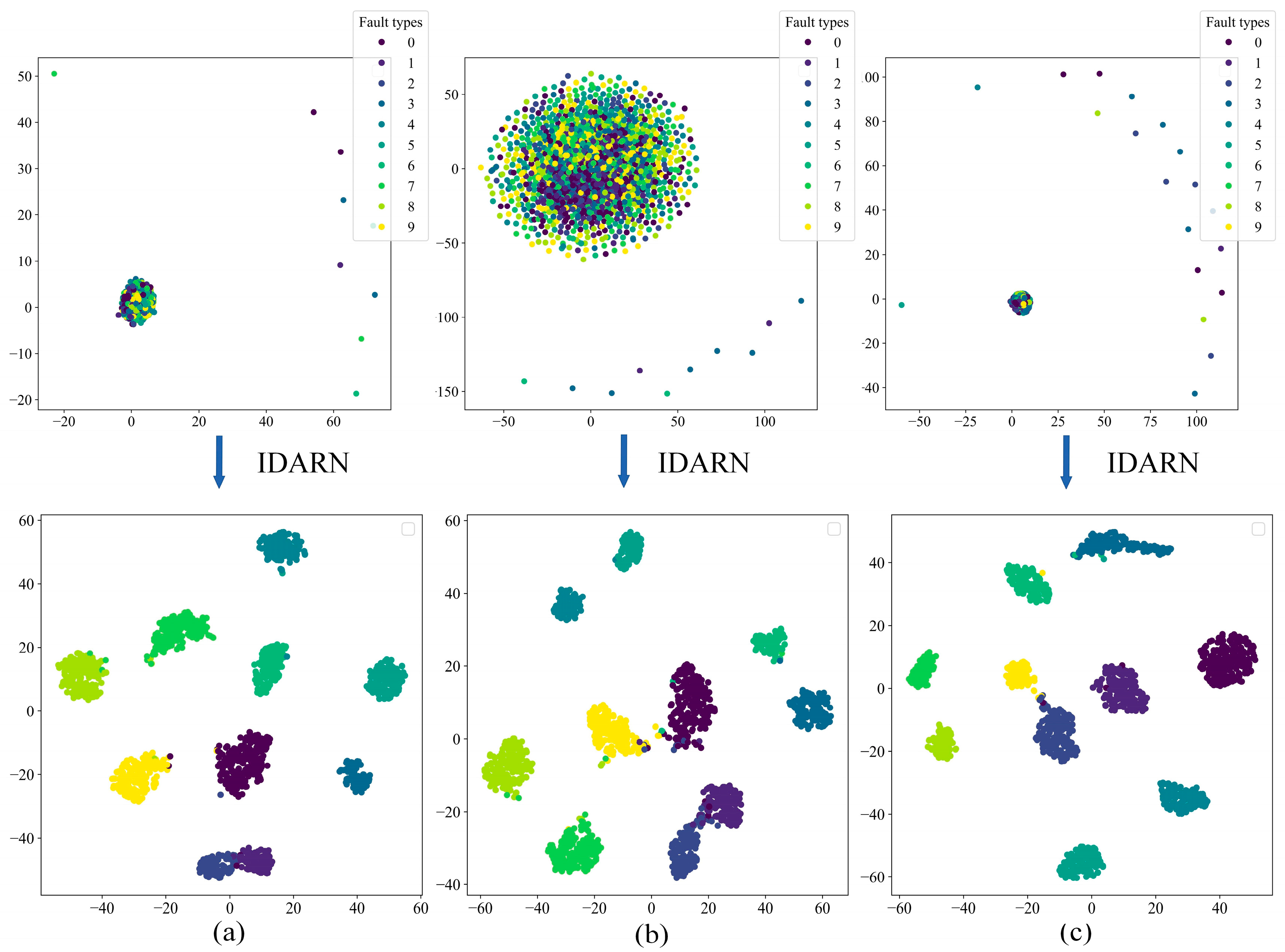
Figure 22.
t-SNE. (a) Dataset1; (b) Dataset2; (c) Dataset3.
Figure 22.
t-SNE. (a) Dataset1; (b) Dataset2; (c) Dataset3.
Table 1.
Summary of literature of data-driven methods models.
Table 1.
Summary of literature of data-driven methods models.
| Ref. | Application | Model | Brief Description | Shortage |
|---|
| [9] | Rolling bearing | WGWOA-VMD-SVM | The proposed method can extract more features. | Difficult to train samples on a large scale. |
| [10] | Gearboxes | VMD-LSTM | Solved EMD modal overlap problem. | Longer calculation time. |
| [11] | Rolling bearing | Spark-IRF | Solve the problems of slower diagnosis speed and repeated voting of traditional RF algorithm. | Overfitting on some noisy classification or regression problems. |
| [12] | Industrial IoT | AutoML | To address the need for bearings to effectively manage predictive maintenance applications. | Not effective when not learning. |
| [13] | Rolling bearing | HPSO-CNN-LSTM | For early fault diagnosis of bearings. | Excessive convolutional layers degrade the network. |
| [14] | Rotating machinery | TCNN | Excellent diagnostic results for small sample data. | Need to pre-train the model. |
| [15] | Rolling bearing | GAF-EDL | For diagnosing data under noise | Not applicable to regression problems. |
| [16,17,18,19] | Rolling bearing | GAF + CNN | To lighten the model and extract more features. | Unstable during training with imbalanced data. |
Table 2.
Commonly used notations.
Table 2.
Commonly used notations.
| Notations | Descriptions |
|---|
| X | One-dimensional time series |
| Polar coordinates of the angle cosine |
| ti | Timestamp |
| N | Constant factor |
| I | Row vector |
| x | Input data |
| H(x) | Residual mapping function |
| F(x) | Constant mapping function |
| M | The size of the batch |
| H | The height of the feature matrices |
| W | The width of the feature matrices |
| C | The number of channels |
| G | Groups of the channels |
| Mean deviation for each group |
| Standard deviation for each group |
| γ | Scale parameter |
| β | Conversion parameter |
| xij | Feature matrices under the channels i and j |
| t | Global aggregated features |
| Weight assigned to each channel |
| Sigmoid function |
| D | 1D convolution operation |
| The closest odd number to the variable |
| b and | Constants |
| S; | The number of neurons on each channel |
| xi | Different neuron |
| The neuron for the input feature of each channel |
| and | The weights and bias values |
| Constant taken as 1 × 10⁻⁴ |
| Q | The number of sampling points |
| Fq | The sampling frequency |
| R | The rotational speed of the bearing |
Table 3.
IDARN model parameters.
Table 3.
IDARN model parameters.
| Disposition | Output Dimension | Layer Design |
|---|
| Input | 224 × 224 × 3 | —— |
| Conv | 112 × 112 × 64 | 7 × 7 × 64, s = 2 |
| Max pool | 56 × 56 × 64 | 3 × 3, s = 2 |
| GN-ECA-1 | 56 × 56 × 64 | |
| GN-ECA-2 | 28 × 28 × 128 | |
| GN-ECA-3 | 14 × 14 × 256 | |
| GN-SimAM | 7 × 7 × 512 | |
| Avg pool | 1 × 1 × 512 | 7 × 7, s = 1 |
| FC | 1 × 1 × 1000 | —— |
| Softmax | 10 | —— |
Table 4.
Division of the datasets.
Table 4.
Division of the datasets.
| Condition | FD/(in) | Label | DatasetA | DatasetB | DatasetC | DatasetD | Train/Val |
|---|
| NO | 0 | 0 | 400 | 400 | 400 | 400 | |
| | 0.007 | 1 | 400 | 100 | 300 | 200 | |
| IF | 0.014 | 2 | 400 | 100 | 300 | 200 | |
| | 0.021 | 3 | 400 | 100 | 300 | 200 | |
| | 0.007 | 4 | 400 | 200 | 100 | 300 | 9/1 |
| RE | 0.014 | 5 | 400 | 200 | 100 | 300 | |
| | 0.021 | 6 | 400 | 200 | 100 | 300 | |
| | 0.007 | 7 | 400 | 300 | 200 | 100 | |
| OF (@6) | 0.014 | 8 | 400 | 300 | 200 | 100 | |
| | 0.021 | 9 | 400 | 300 | 200 | 100 | |
Table 5.
Network training parameters.
Table 5.
Network training parameters.
| Pre-Processing Method | Batch Size | Loss Function | Optimizer | Learn Rate |
|---|
| Random Horizon Filp | | | | |
| Random Resize Crop | 8 | Crossentropy Loss | Adam | 0.0001 |
| Normalize | | | | |
Table 6.
Accuracy of different normalisation methods.
Table 6.
Accuracy of different normalisation methods.
| Dataset/Method | BN/(%) | GN-4/(%) | GN-8/(%) | GN-16/(%) |
|---|
| DatasetA | 99.3 | 99.3 | 99.5 | 99 |
| DatasetB | 98.1 | 98.8 | 99.1 | 98.6 |
| DatasetC | 97.5 | 98.1 | 98.6 | 98.6 |
| DatasetD | 98.6 | 99.1 | 99.5 | 99.1 |
Table 7.
Accuracy of different attention methods.
Table 7.
Accuracy of different attention methods.
| Dataset/Method | CARN/(%) | SARN/(%) | DARN/(%) |
|---|
| DatasetA | 99.5 | 99.3 | 99.5 |
| DatasetB | 98.6 | 98.8 | 99.1 |
| DatasetC | 98.6 | 98.1 | 98.6 |
| DatasetD | 99.1 | 99.2 | 99.5 |
Table 8.
Comparative accuracy in validation set.
Table 8.
Comparative accuracy in validation set.
| Method/Dataset | DatasetA/(%) | DatasetB/(%) | DatasetC/(%) | DatasetD/(%) |
|---|
| GADF-EDL [15] | 99 | 98.6 | 98.2 | 98.2 |
| GADF-DenseNet [16] | 99.5 | 98.2 | 98.6 | 99.1 |
| GADF-FcaNet [17] | 99.3 | 98.2 | 98.2 | 98.6 |
| GADF-CAnet [18] | 99 | 98.6 | 97.7 | 98.2 |
| GADF-ResNeXt50 [19] | 98.5 | 97.7 | 98.2 | 98.6 |
| GADF-IDARN | 99.5 | 99.1 | 98.6 | 99.5 |
Table 9.
Comparative indicators in DatasetA.
Table 9.
Comparative indicators in DatasetA.
| Method | Pr (Avg) | Re (Avg) | F1 | Train Time/Epoch |
|---|
| GADF-EDL | 0.9894 | 0.9902 | 0.9898 | 106 s |
| GADF-DenseNet | 0.9952 | 0.9950 | 0.9951 | 145 s |
| GADF-FcaNet | 0.9926 | 0.9925 | 0.9925 | 108 s |
| GADF-CAnet | 0.9904 | 0.9900 | 0.9901 | 111 s |
| GADF-ResNeXt50 | 0.9856 | 0.9850 | 0.9853 | 266 s |
| GADF-IDARN | 0.9950 | 0.9950 | 0.9950 | 96 s |
Table 10.
Comparative indicators in DatasetB.
Table 10.
Comparative indicators in DatasetB.
| Method | Pr (Avg) | Re (Avg) | F1 | Train Time/Epoch |
|---|
| GADF-EDL | 0.9887 | 0.9817 | 0.9852 | 62 s |
| GADF-DenseNet | 0.9714 | 0.9867 | 0.9790 | 94 s |
| GADF-FcaNet | 0.9714 | 0.9800 | 0.9757 | 63 s |
| GADF-CAnet | 0.9853 | 0.9824 | 0.9838 | 83 s |
| GADF-ResNeXt50 | 0.9733 | 0.9733 | 0.9733 | 146 s |
| GADF-IDARN | 0.9920 | 0.9833 | 0.9876 | 54 s |
Table 11.
Comparative indicators in DatasetC.
Table 11.
Comparative indicators in DatasetC.
| Method | Pr (Avg) | Re (Avg) | F1 | Train Time/Epoch |
|---|
| GADF-EDL | 0.9853 | 0.9750 | 0.9801 | 62 s |
| GADF-DenseNet | 0.9885 | 0.9817 | 0.9851 | 94 s |
| GADF-FcaNet | 0.9809 | 0.9850 | 0.9829 | 63 s |
| GADF-CAnet | 0.9747 | 0.9703 | 0.9725 | 83 s |
| GADF-ResNeXt50 | 0.9818 | 0.9800 | 0.9809 | 146 s |
| GADF-IDARN | 0.9871 | 0.9883 | 0.9877 | 54 s |
Table 12.
Comparative indicators in DatasetD.
Table 12.
Comparative indicators in DatasetD.
| Method | Pr (Avg) | Re (Avg) | F1 | Train Time/Epoch |
|---|
| GADF-EDL | 0.9847 | 0.9809 | 0.9828 | 62 s |
| GADF-DenseNet | 0.9909 | 0.9933 | 0.9921 | 94 s |
| GADF-FcaNet | 0.9887 | 0.9803 | 0.9845 | 63 s |
| GADF-CAnet | 0.9853 | 0.9824 | 0.9838 | 83 s |
| GADF-ResNeXt50 | 0.9885 | 0.9824 | 0.9854 | 146 s |
| GADF-IDARN | 0.9968 | 0.9967 | 0.9967 | 54 s |
Table 13.
Comparative results.
Table 13.
Comparative results.
| Method | Classification Category | Accuracy (%) |
|---|
| 1D-CNN [25] | 6 | 93.2 |
| CNNEPDNN [26] | 10 | 97.85 |
| LSTM-1DCNN [27] | 10 | 98.46 |
| MTF-ResNet [28] | 10 | 98.52 |
| ResNet-LSTM [29] | 10 | 98.95 |
| IDARN | 10 | 99.5 |
Table 14.
Data division.
| Condition | Rpm | Label | Dataset1 | Dataset2 | Dataset3 | Train/Val |
|---|
| NO | 1000 | 0 | 250 | 250 | 250 | |
| | 500 | 1 | 100 | 150 | 200 | |
| IF | 1000 | 2 | 100 | 150 | 200 | |
| | 1500 | 3 | 100 | 150 | 200 | |
| | 500 | 4 | 150 | 100 | 150 | 9/1 |
| OF | 1000 | 5 | 150 | 100 | 150 | |
| | 1500 | 6 | 150 | 100 | 150 | |
| | 500 | 7 | 200 | 200 | 100 | |
| RE | 1000 | 8 | 200 | 200 | 100 | |
| | 1500 | 9 | 200 | 200 | 100 | |
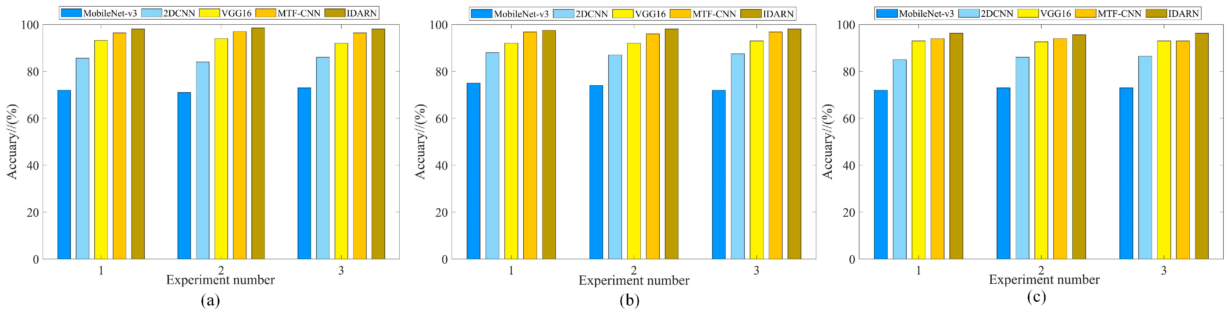
Table 15.
Accuracy of different methods.
Table 15.
Accuracy of different methods.
| Dataset/Method | Mobilenet-v3/% | 2DCNN/% | VGG16/% | MTF-CNN/% | IDARN/% |
|---|
| Dataset1 | 71.9 | 85.6 | 94.6 | 97 | 98.8 |
| Dataset2 | 74 | 87.2 | 92.8 | 96.4 | 98.1 |
| Dataset3 | 70.7 | 83.8 | 93.4 | 94 | 96.9 |
Table 16.
Comparative indicators of popular CNN models in Dataset1.
Table 16.
Comparative indicators of popular CNN models in Dataset1.
| Method | Pr (Avg) | Re (Avg) | F1 | Train Time/Epoch |
|---|
| Mobilenet-v3 | 0.7293 | 0.7175 | 0.7233 | 17 s |
| 2DCNN | 0.8493 | 0.8300 | 0.8395 | 35 s |
| VGG16 | 0.9414 | 0.9093 | 0.9251 | 26 s |
| MTF-CNN | 0.9684 | 0.9726 | 0.9704 | 57 s |
| IDARN | 0.9904 | 0.9800 | 0.9852 | 37 s |
Table 17.
Comparative indicators of popular CNN models in Dataset2.
Table 17.
Comparative indicators of popular CNN models in Dataset2.
| Method | Pr (Avg) | Re (Avg) | F1 | Train Time/Epoch |
|---|
| Mobilenet-v3 | 0.7526 | 0.7367 | 0.7446 | 17 s |
| 2DCNN | 0.8633 | 0.8468 | 0.8550 | 35 s |
| VGG16 | 0.9307 | 0.9169 | 0.9237 | 26 s |
| MTF-CNN | 0.9749 | 0.9603 | 0.9675 | 57 s |
| IDARN | 0.9833 | 0.9800 | 0.9816 | 37 s |
Table 18.
Comparative indicators of popular CNN models in Dataset3.
Table 18.
Comparative indicators of popular CNN models in Dataset3.
| Method | Pr (Avg) | Re (Avg) | F1 | Train Time/Epoch |
|---|
| Mobilenet-v3 | 0.7149 | 0.7056 | 0.7102 | 17 s |
| 2DCNN | 0.8267 | 0.8347 | 0.8307 | 35 s |
| VGG16 | 0.9252 | 0.9336 | 0.9294 | 26 s |
| MTF-CNN | 0.9537 | 0.9430 | 0.9483 | 57 s |
| IDARN | 0.9733 | 0.9700 | 0.9716 | 37 s |
Table 19.
Comparative Indicators of related models in Dataset1.
Table 19.
Comparative Indicators of related models in Dataset1.
| Method | Accuracy (%) | Pr (Avg) | Re (Avg) | F1 | Train Time/Epoch |
|---|
| GADF-EDL | 97.7 | 0.9756 | 0.9700 | 0.9728 | 45 s |
| GADF-DenseNet | 98.1 | 0.9816 | 0.9749 | 0.9782 | 53 s |
| GADF-FcaNet | 97 | 0.9747 | 0.9667 | 0.9707 | 44 s |
| GADF-CAnet | 96.9 | 0.9696 | 0.9567 | 0.9631 | 48 s |
| GADF-ResNeXt50 | 95.6 | 0.9633 | 0.9566 | 0.9599 | 107 s |
| GADF-IDARN | 98.8 | 0.9904 | 0.9800 | 0.9852 | 37 s |
Table 20.
Comparative Indicators of related models in Dataset2.
Table 20.
Comparative Indicators of related models in Dataset2.
| Method | Accuracy (%) | Pr (Avg) | Re (Avg) | F1 | Train Time/Epoch |
|---|
| GADF-EDL | 96.3 | 0.9605 | 0.9493 | 0.9549 | 45 s |
| GADF-DenseNet | 98.1 | 0.9826 | 0.9733 | 0.9779 | 53 s |
| GADF-FcaNet | 95.6 | 0.9449 | 0.9383 | 0.9416 | 44 s |
| GADF-CAnet | 97.5 | 0.9707 | 0.9660 | 0.9683 | 48 s |
| GADF-ResNeXt50 | 95 | 0.9507 | 0.9220 | 0.9361 | 107 s |
| GADF-IDARN | 98.1 | 0.9833 | 0.9800 | 0.9816 | 37 s |
Table 21.
Comparative Indicators of related models in Dataset3.
Table 21.
Comparative Indicators of related models in Dataset3.
| Method | Accuracy (%) | Pr (Avg) | Re (Avg) | F1 | Train Time/Epoch |
|---|
| GADF-EDL | 93.1 | 0.9409 | 0.9403 | 0.9406 | 45 s |
| GADF-DenseNet | 95.6 | 0.9665 | 0.9650 | 0.9657 | 53 s |
| GADF-FcaNet | 94.4 | 0.9538 | 0.9550 | 0.9544 | 44 s |
| GADF-CAnet | 95.6 | 0.9652 | 0.9650 | 0.9651 | 48 s |
| GADF-ResNeXt50 | 92.5 | 0.9252 | 0.9393 | 0.9322 | 107 s |
| GADF-IDARN | 96.9 | 0.9733 | 0.9700 | 0.9716 | 37 s |


