
Utilization of Synthetic Near-Infrared Spectra via Generative Adversarial Network to Improve Wood Stiffness Prediction

 ,
,  ,
, 
 , ,
, ,  and
and
Abstract
1. Introduction
2. Materials and Methods
2.1. Materials
2.2. NIR Spectral Data Collection
2.3. Data Augmentation Using Generative Adversarial Network (GAN)
2.4. Model Fitting
2.5. Hyperparameter Tuning, Model Training, and Evaluation
3. Results and Discussions
4. Conclusions
Author Contributions
Funding
Institutional Review Board Statement
Informed Consent Statement
Data Availability Statement
Conflicts of Interest
References
- Schimleck, L.; Dahlen, J.; Apiolaza, L.A.; Downes, G.; Emms, G.; Evans, R.; Moore, J.; Pâques, L.; Van den Bulcke, J.; Wang, X. Non-destructive evaluation techniques and what they tell us about wood property variation. Forests 2019, 10, 728. [Google Scholar] [CrossRef]
- Nasir, V.; Ayanleye, S.; Kazemirad, S.; Sassani, F.; Adamopoulos, S. Acoustic emission monitoring of wood materials and timber structures: A critical review. Constr. Build. Mater. 2022, 350, 128877. [Google Scholar] [CrossRef]
- Tsuchikawa, S.; Kobori, H. A review of recent application of near infrared spectroscopy to wood science and technology. J. Wood Sci. 2015, 61, 213–220. [Google Scholar] [CrossRef]
- Willems, W.; Lykidis, C.; Altgen, M.; Clauder, L. Quality control methods for thermally modified wood: COST action FP0904 2010–2014: Thermo-hydro-mechanical wood behaviour and processing. Holzforschung 2015, 69, 875–884. [Google Scholar] [CrossRef]
- Tsuchikawa, S. A review of recent near infrared research for wood and paper. Appl. Spectrosc. Rev. 2007, 42, 43–71. [Google Scholar] [CrossRef]
- Tsuchikawa, S.; Schwanninger, M. A review of recent near-infrared research for wood and paper (Part 2). Appl. Spectrosc. Rev. 2013, 48, 560–587. [Google Scholar] [CrossRef]
- Sandak, J.; Sandak, A.; Meder, R. Assessing trees, wood and derived products with near infrared spectroscopy: Hints and tips. J. Near. Infrared Spectrosc. 2016, 24, 485–505. [Google Scholar] [CrossRef]
- Schimleck, L.R.; Matos, J.L.M.; Trianoski, R.; Prata, J.G. Comparison of methods for estimating mechanical properties of wood by NIR spectroscopy. J. Spectrosc. 2018, 2018, 4823285. [Google Scholar] [CrossRef]
- Hoffmeyer, P.; Pedersen, J. Evaluation of density and strength of Norway spruce wood by near-infrared reflectance spectroscopy. Holz Roh Werkst 1995, 53, 165–170. [Google Scholar] [CrossRef]
- Haartveit, E.Y.; Flæte, P.O. Rapid prediction of basic wood properties by near infrared spectroscopy. N. Z. J. For. Sci. 2006, 36, 393–407. [Google Scholar]
- Thumm, A.; Meder, R. Stiffness prediction of radiata pine clearwood test pieces using near infrared spectroscopy. J. Near Infrared Spectrosc. 2001, 9, 117–122. [Google Scholar] [CrossRef]
- Kelley, S.S.; Rials, T.G.; Snell, R.; Groom, L.H.; Sluiter, A. Use of near infrared spectroscopy to measure the chemical and mechanical properties of solid wood. Wood Sci. Technol. 2004, 38, 257–276. [Google Scholar] [CrossRef]
- Schimleck, L.R.; Jones, P.D.; Clark, A.; Daniels, R.F.; Peter, G.F. Near infrared spectroscopy for the nondestructive estimation of clear wood properties of Pinus taeda L. from the southern United States. For. Prod. J. 2005, 55, 21–28. [Google Scholar]
- Via, B.K.; So, C.L.; Shupe, T.F.; Eckhardt, L.G.; Stine, M.; Groom, L.H. Prediction of wood mechanical and chemical properties in the presence and absence of blue stain using two near infrared instruments. J. Near Infrared Spectrosc. 2005, 13, 201–212. [Google Scholar] [CrossRef]
- Via, B.K.; Shupe, T.F.; Groom, L.H.; Stine, M.; So, C.L. Multivariate modelling of density, strength and stiffness from near infrared spectra for mature, juvenile and pith wood of longleaf pine (Pinus palustris). J. Near Infrared Spectrosc. 2003, 11, 365–378. [Google Scholar] [CrossRef]
- Fujimoto, T.; Yamamoto, H.; Tsuchikawa, S. Estimation of wood stiffness and strength properties of hybrid larch by near-infrared spectroscopy. Appl. Spectrosc. 2007, 61, 882–888. [Google Scholar] [CrossRef]
- Fujimoto, T.; Kurata, Y.; Matsumoto, K.; Tsuchikawa, S. Application of near infrared spectroscopy for estimating wood mechanical properties of small clear and full length lumber specimens. J. Near Infrared Spectrosc. 2008, 16, 529–537. [Google Scholar] [CrossRef]
- Dahlen, J.; Diaz, I.; Schimleck, L.; Jones, P.D. Near-infrared spectroscopy prediction of southern pine No. 2 lumber physical and mechanical properties. Wood Sci. Technol. 2017, 51, 309–322. [Google Scholar] [CrossRef]
- Schimleck, L.R.; Evans, R.; Ilic, J. Estimation of Eucalyptus delegatensis wood properties by near infrared spectroscopy. Can. J. For. Res. 2001, 31, 1671–1675. [Google Scholar] [CrossRef]
- Kothiyal, V.; Raturi, A. Estimating mechanical properties and specific gravity for five-year-old Eucalyptus tereticornis having broad moisture content range by NIR spectroscopy. Holzforschung 2011, 65, 757–762. [Google Scholar] [CrossRef]
- Zhao, R.; Huo, X.; Zhang, L. Estimation of modulus of elasticity of Eucalyptus pellita wood by near infrared spectroscopy. Spectrosc. Spectr. Anal. 2009, 29, 2392–2395. [Google Scholar]
- Miotto, R.; Wang, F.; Wang, S.; Jiang, X.; Dudley, J.T. Deep learning for healthcare: Review, opportunities and challenges. Brief. Bioinform. 2018, 19, 1236–1246. [Google Scholar] [CrossRef] [PubMed]
- Wang, J.; Ma, Y.; Zhang, L.; Gao, R.X.; Wu, D. Deep learning for smart manufacturing: Methods and applications. J. Manuf. Syst. 2018, 48, 144–156. [Google Scholar] [CrossRef]
- Watanabe, K.; Kobayashi, I.; Matsushita, Y.; Saito, S.; Kuroda, N.; Noshiro, S. Application of near-infrared spectroscopy for evaluation of drying stress on lumber surface: A comparison of artificial neural networks and partial least squares regression. Dry. Technol. 2014, 32, 590–596. [Google Scholar] [CrossRef]
- Costa, L.R.; Tonoli, G.H.D.; Milagres, F.R.; Hein, P.R.G. Artificial neural network and partial least square regressions for rapid estimation of cellulose pulp dryness based on near infrared spectroscopic data. Carbohydr. Polym. 2019, 224, 115186. [Google Scholar] [CrossRef] [PubMed]
- Ayanleye, S.; Nasir, V.; Avramidis, S.; Cool, J. Effect of wood surface roughness on prediction of structural timber properties by infrared spectroscopy using ANFIS, ANN and PLS regression. Eur. J. Wood Wood Prod. 2021, 79, 101–115. [Google Scholar] [CrossRef]
- Nasir, V.; Ali, S.D.; Mohammadpanah, A.; Raut, S.; Nabavi, M.; Dahlen, J.; Schimleck, L. Fiber quality prediction using NIR spectral data: Tree-based ensemble learning vs. deep neural networks. Wood Fiber Sci. 2023, 55, 100–115. [Google Scholar] [CrossRef]
- Nasir, V.; Nourian, S.; Zhou, Z.; Rahimi, S.; Avramidis, S.; Cool, J. Classification and characterization of thermally modified timber using visible and near-infrared spectroscopy and artificial neural networks: A comparative study on the performance of different NDE methods and ANNs. Wood Sci. Technol. 2019, 53, 1093–1109. [Google Scholar] [CrossRef]
- Grinsztajn, L.; Oyallon, E.; Varoquaux, G. Why do tree-based models still outperform deep learning on typical tabular data? In Advances in Neural Information Processing Systems; Koyejo, S., Mohamed, S., Agarwal, A., Belgrave, D., Cho, K., Oh, A., Eds.; Curran Associates, Inc.: Red Hook, NY, USA, 2022; pp. 507–520. [Google Scholar] [CrossRef]
- Lamb, A. A brief introduction to generative models. arXiv 2021, arXiv:2103.00265. [Google Scholar] [CrossRef]
- Goodfellow, I.; Pouget-Abadie, J.; Mirza, M.; Xu, B.; Warde-Farley, D.; Ozair, S.; Courville, A.; Bengio, Y. Generative adversarial nets. In Advances in Neural Information Processing Systems; Ghahramani, Z., Welling, M., Cortes, C., Lawrence, N., Weinberger, K.Q., Eds.; Curran Associates, Inc.: Red Hook, NY, USA, 2014; pp. 2672–2680. [Google Scholar]
- Nagasawa, T.; Sato, T.; Nambu, I.; Wada, Y. fNIRS-GANs: Data augmentation using generative adversarial networks for classifying motor tasks from functional near-infrared spectroscopy. J. Neural Eng. 2020, 17, 016068. [Google Scholar] [CrossRef]
- Zhang, Y.; Gan, Z.; Fan, K.; Chen, Z.; Henao, R.; Shen, D.; Carin, L. Adversarial feature matching for text generation. In Proceedings of the 34th International Conference on Machine Learning, Sydney, Australia, 6–11 August 2017; Precup, D., Teh, Y.W., Eds.; PMLR, ML Research Press: Maastricht, The Netherlands, 2017; pp. 4006–4015. [Google Scholar]
- Engel, J.; Agrawal, K.K.; Chen, S.; Gulrajani, I.; Donahue, C.; Roberts, A. GANSynth: Adversarial neural audio synthesis. arXiv 2019, arXiv:1902.08710. [Google Scholar]
- Zhang, L.; Wang, Y.; Wei, Y.; An, D. Near-infrared hyperspectral imaging technology combined with deep convolutional generative adversarial network to predict oil content of single maize kernel. Food Chem. 2022, 370, 131047. [Google Scholar] [CrossRef] [PubMed]
- Little, C.; Elliot, M.; Allmendinger, R.; Samani, S.S. Generative adversarial networks for synthetic data generation: A comparative study. arXiv 2021, arXiv:2112.01925. [Google Scholar] [CrossRef]
- Smith, K.E.; Smith, A.O. Conditional GAN for timeseries generation. arXiv 2020, arXiv:2006.16477. [Google Scholar] [CrossRef]
- Hu, J.; Yang, H.; Zhao, G.; Zhou, R. Research on online rapid sorting method of waste textiles based on near-infrared spectroscopy and generative adversity network. Comput. Intell. Neurosci. 2022, 2022, 6215101. [Google Scholar] [CrossRef]
- Zhu, D.; Xu, L.; Chen, X.; Yuan, L.; Huang, G.; Li, L.; Chen, X.; Shi, W. Synthetic spectra generated by boundary equilibrium generative adversarial networks and their applications with consensus algorithms. Opt. Express 2020, 28, 17196–17208. [Google Scholar] [CrossRef]
- Teng, G.E.; Wang, Q.Q.; Kong, J.L.; Dong, L.Q.; Cui, X.T.; Liu, W.W.; Wei, K.; Xiangli, W.T. Extending the spectral database of laser-induced breakdown spectroscopy with generative adversarial nets. Opt. Express 2019, 27, 6958–6969. [Google Scholar] [CrossRef]
- Yang, B.; Chen, C.; Chen, F.; Chen, C.; Tang, J.; Gao, R.; Lv, X. Identification of cumin and fennel from different regions based on generative adversarial networks and near infrared spectroscopy. Spectrochim. Acta—Part A Mol. Biomol. Spectrosc. 2021, 260, 119956. [Google Scholar] [CrossRef] [PubMed]
- Li, H.; Zhang, L.; Sun, H.; Rao, Z.; Ji, H. Discrimination of unsound wheat kernels based on deep convolutional generative adversarial network and near-infrared hyperspectral imaging technology. Spectrochim. Acta—Part A Mol. Biomol. Spectrosc. 2022, 268, 120722. [Google Scholar] [CrossRef]
- Zheng, A.; Yang, H.; Pan, X.; Yin, L.; Feng, Y. Identification of multi-class drugs based on near infrared spectroscopy and bidirectional generative adversarial networks. Sensors 2021, 21, 1088. [Google Scholar] [CrossRef]
- Dahlen, J.; Jones, P.D.; Seale, R.D.; Shmulsky, R. Mill variation in bending strength and stiffness of in-grade southern pine No. 2 2 × 4 lumber. Wood Sci. Technol. 2013, 47, 1153–1165. [Google Scholar] [CrossRef]
- ASTM International, D198-15; Standard Test Methods of Static Tests of Lumber in Structural Sizes. ASTM International: West Conshohocken, PA, USA, 2015.
- ASTM International, D1990-16; Standard Practice for Establishing Allowable Properties for Visually-Graded Dimension Lumber from In-Grade Tests of Full-Size Specimens. ASTM International: West Conshohocken, PA, USA, 2016.
- Savitzky, A.; Golay, M.J. Smoothing and differentiation of data by simplified least squares procedures. Anal. Chem. 1964, 36, 1627–1639. [Google Scholar] [CrossRef]
- Wu, M.; Wang, S.; Pan, S.; Terentis, A.C.; Strasswimmer, J.; Zhu, X. Deep learning data augmentation for Raman spectroscopy cancer tissue classification. Sci. Rep. 2021, 11, 23842. [Google Scholar] [CrossRef] [PubMed]
- Liu, X.; Qiao, Y.; Xiong, Y.; Cai, Z.; Liu, P. Cascade conditional generative adversarial nets for spatial-spectral hyperspectral sample generation. Sci. China Inf. Sci. 2020, 63, 140306. [Google Scholar] [CrossRef]
- Fernandes, A.; Lousada, J.; Morais, J.; Xavier, J.; Pereira, J.; Melo-Pinto, P. Comparison between neural networks and partial least squares for intra-growth ring wood density measurement with hyperspectral imaging. Comput. Electron. Agric. 2013, 94, 71–81. [Google Scholar] [CrossRef]
- Gu, J.; Wang, Z.; Kuen, J.; Ma, L.; Shahroudy, A.; Shuai, B.; Liu, T.; Wang, X.; Wang, G.; Cai, J.; et al. Recent advances in convolutional neural networks. Pattern Recognit. 2018, 77, 354–377. [Google Scholar] [CrossRef]
- Lecun, Y.; Bengio, Y.; Hinton, G. Deep learning. Nature 2015, 521, 436–444. [Google Scholar] [CrossRef]
- Ke, G.; Meng, Q.; Finley, T.; Wang, T.; Chen, W.; Ma, W.; Ye, Q.; Liu, T.-Y. LightGBM: A highly efficient gradient boosting decision tree. In Advances in Neural Information Processing System; Guyon, I., Von Luxburg, U., Bengio, S., Wallach, H., Fergus, R., Vishwanathan, S., Garnett, R., Eds.; Curran Associates, Inc.: Red Hook, NY, USA, 2017; Available online: https://proceedings.neurips.cc/paper_files/paper/2017/file/6449f44a102fde848669bdd9eb6b76fa-Paper.pdf (accessed on 5 March 2023).
- Guo, J.; Yun, S.; Meng, Y.; He, N.; Ye, D.; Zhao, Z.; Jia, L.; Yang, L. Prediction of heating and cooling loads based on light gradient boosting machine algorithms. Build. Environ. 2023, 236, 110252. [Google Scholar] [CrossRef]
- Akiba, T.; Sano, S.; Yanase, T.; Ohta, T.; Koyama, M. Optuna: A next-generation hyperparameter optimization framework. In Proceedings of the 25th ACM SIGKDD International Conference on Knowledge Discovery & Data Mining (KDD ’19), Anchorage, AK, USA, 4–8 August 2019; pp. 2623–2631. [Google Scholar] [CrossRef]
- R Core Team. R: A Language and Environment for Statistical Computing; R Foundation for Statistical Computing: Vienna, Austria, 2023; Available online: https://www.R-project.org/ (accessed on 1 March 2023).
- RStudio. RStudio: Integrated Development for R.; RStudio, Inc.: Boston, MA, USA, 2023; Available online: http://www.rstudio.com/ (accessed on 1 March 2023).
- Wickham, H. ggplot2: Elegant Graphics for Data Analysis; Springer: New York, NY, USA, 2016. [Google Scholar]
- Hwang, Y.; Song, J. Recent deep learning methods for tabular data. Commun. Stat. Appl. Methods 2023, 30, 215–226. [Google Scholar] [CrossRef]
- Schimleck, L.; Ma, T.; Inagaki, T.; Tsuchikawa, S. Review of near infrared hyperspectral imaging applications related to wood and wood products. Appl. Spectrosc. Rev. 2023, 58, 585–609. [Google Scholar] [CrossRef]


| Dataset | Min | 1st Quartile | Median | Mean | 3rd Quartile | Max |
|---|---|---|---|---|---|---|
| Training dataset MOE (GPa) (N = 573) | 3.577 | 8.579 | 10.529 | 10.920 | 13.112 | 21.761 |
| Test dataset MOE (GPa) (N = 145) | 3.211 | 8.771 | 10.913 | 11.129 | 13.600 | 22.040 |
| Enhanced Training dataset MOE (GPa) (N = 573 + 313) | 3.577 | 9.259 | 10.400 | 10.706 | 11.864 | 21.761 |
| Enhanced Training dataset MOE (GPa) (N = 573 + 573) | 3.577 | 9.779 | 10.614 | 10.897 | 12.886 | 21.761 |
| Enhanced Training dataset MOE (GPa) (N = 573 + 1000) | 3.577 | 8.028 | 8.473 | 9.608 | 10.415 | 21.761 |
| Model | Property | Train R2 | Test R2 | Train RMSE (GPa) | Test RMSE (GPa) |
|---|---|---|---|---|---|
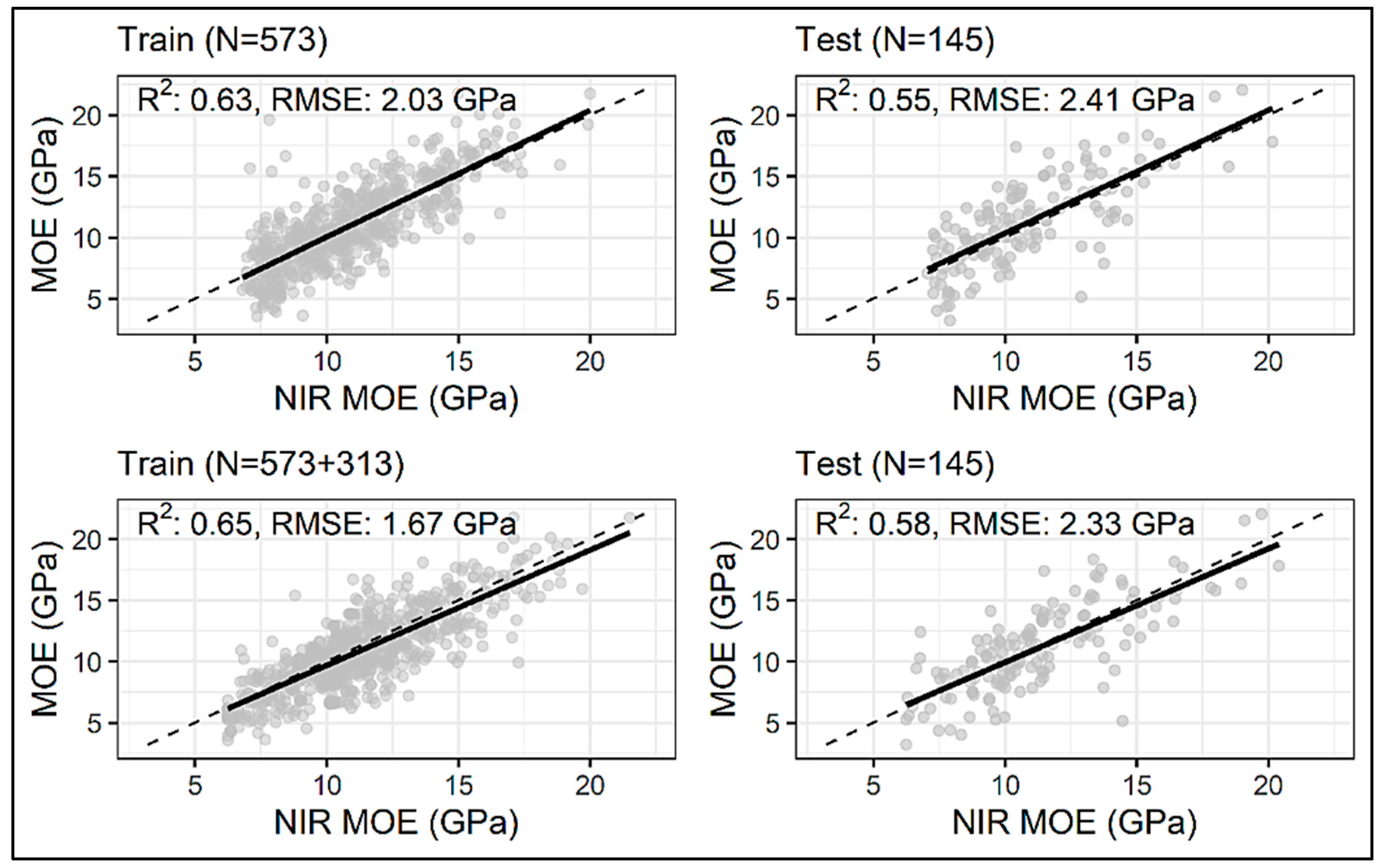
| ANN | MOE Original (N = 573) | 0.63 | 0.55 | 2.03 | 2.41 |
| MOE Enhanced (N = 573 + 313) | 0.65 | 0.58 | 1.67 | 2.33 | |
| MOE Enhanced (N = 573 + 573) | 0.68 | 0.56 | 1.56 | 2.38 | |
| MOE Enhanced (N = 573 + 1000) | 0.66 | 0.56 | 1.48 | 2.38 | |
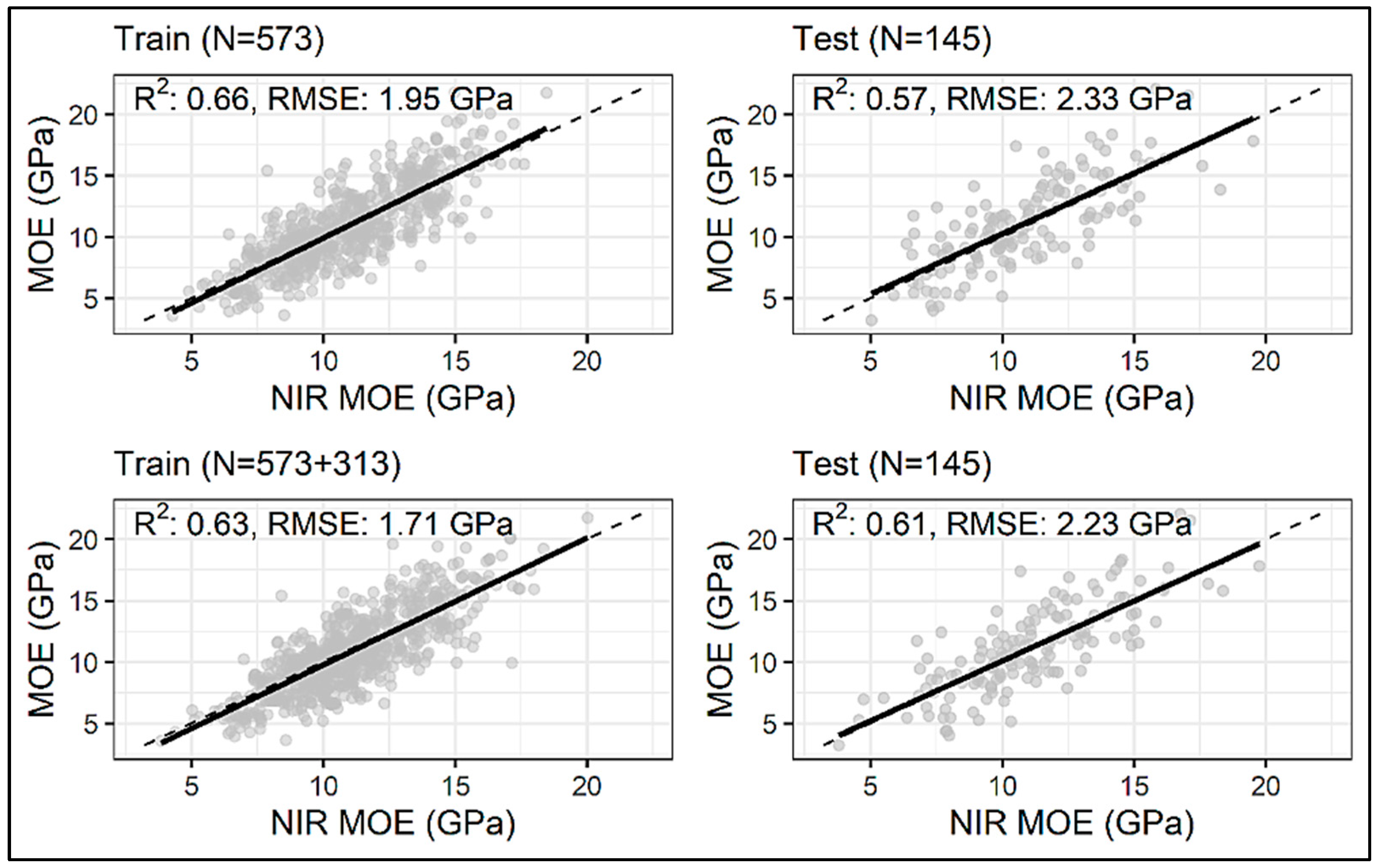
| CNN | MOE Original (N = 573) | 0.66 | 0.57 | 1.95 | 2.33 |
| MOE Enhanced (N = 573 + 313) | 0.63 | 0.61 | 1.71 | 2.23 | |
| MOE Enhanced (N = 573 + 573) | 0.58 | 0.58 | 1.76 | 2.31 | |
| MOE Enhanced (N = 573 + 1000) | 0.65 | 0.58 | 1.50 | 2.31 | |
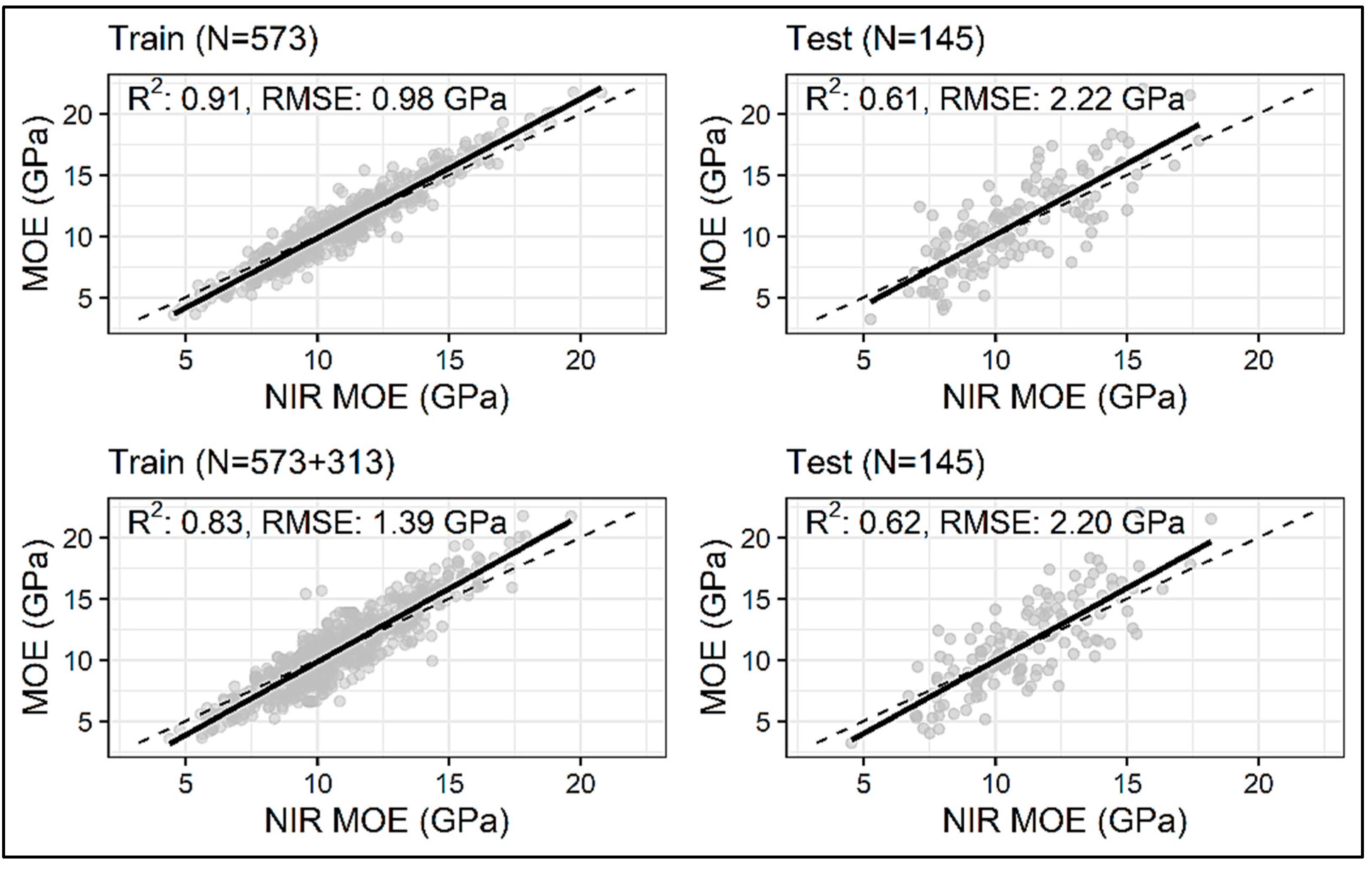
| LGBM | MOE Original (N = 573) | 0.91 | 0.61 | 0.98 | 2.22 |
| MOE Enhanced (N = 573 + 313) | 0.83 | 0.62 | 1.39 | 2.20 | |
| MOE Enhanced (N = 573 + 573) | 0.72 | 0.61 | 1.77 | 2.22 | |
| MOE Enhanced (N = 573 + 1000) | 0.74 | 0.60 | 1.29 | 2.24 |
Disclaimer/Publisher’s Note: The statements, opinions and data contained in all publications are solely those of the individual author(s) and contributor(s) and not of MDPI and/or the editor(s). MDPI and/or the editor(s) disclaim responsibility for any injury to people or property resulting from any ideas, methods, instructions or products referred to in the content. |
© 2024 by the authors. Licensee MDPI, Basel, Switzerland. This article is an open access article distributed under the terms and conditions of the Creative Commons Attribution (CC BY) license (https://creativecommons.org/licenses/by/4.0/).
Share and Cite
Ali, S.D.; Raut, S.; Dahlen, J.; Schimleck, L.; Bergman, R.; Zhang, Z.; Nasir, V. Utilization of Synthetic Near-Infrared Spectra via Generative Adversarial Network to Improve Wood Stiffness Prediction. Sensors 2024, 24, 1992. https://doi.org/10.3390/s24061992
Ali SD, Raut S, Dahlen J, Schimleck L, Bergman R, Zhang Z, Nasir V. Utilization of Synthetic Near-Infrared Spectra via Generative Adversarial Network to Improve Wood Stiffness Prediction. Sensors. 2024; 24(6):1992. https://doi.org/10.3390/s24061992
Chicago/Turabian StyleAli, Syed Danish, Sameen Raut, Joseph Dahlen, Laurence Schimleck, Richard Bergman, Zhou Zhang, and Vahid Nasir. 2024. "Utilization of Synthetic Near-Infrared Spectra via Generative Adversarial Network to Improve Wood Stiffness Prediction" Sensors 24, no. 6: 1992. https://doi.org/10.3390/s24061992
APA StyleAli, S. D., Raut, S., Dahlen, J., Schimleck, L., Bergman, R., Zhang, Z., & Nasir, V. (2024). Utilization of Synthetic Near-Infrared Spectra via Generative Adversarial Network to Improve Wood Stiffness Prediction. Sensors, 24(6), 1992. https://doi.org/10.3390/s24061992