
Three-Dimensional Reconstruction and Deformation Identification of Slope Models Based on Structured Light Method


Abstract
1. Introduction
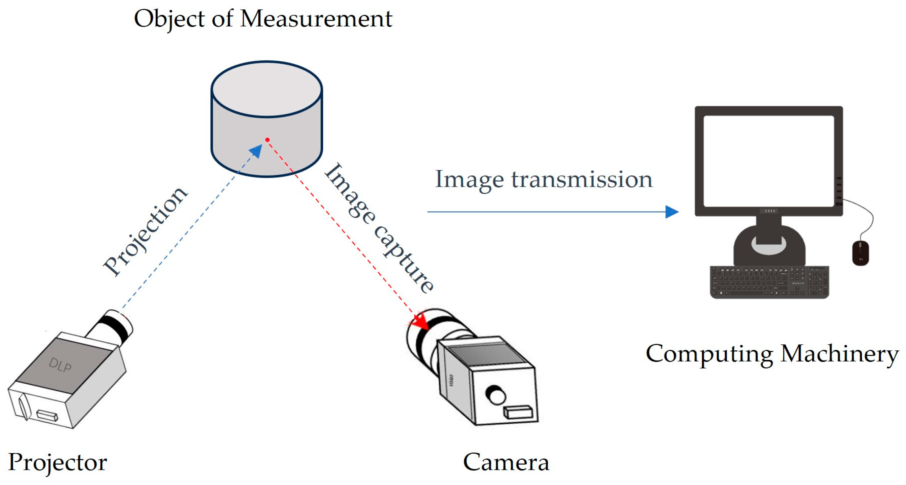
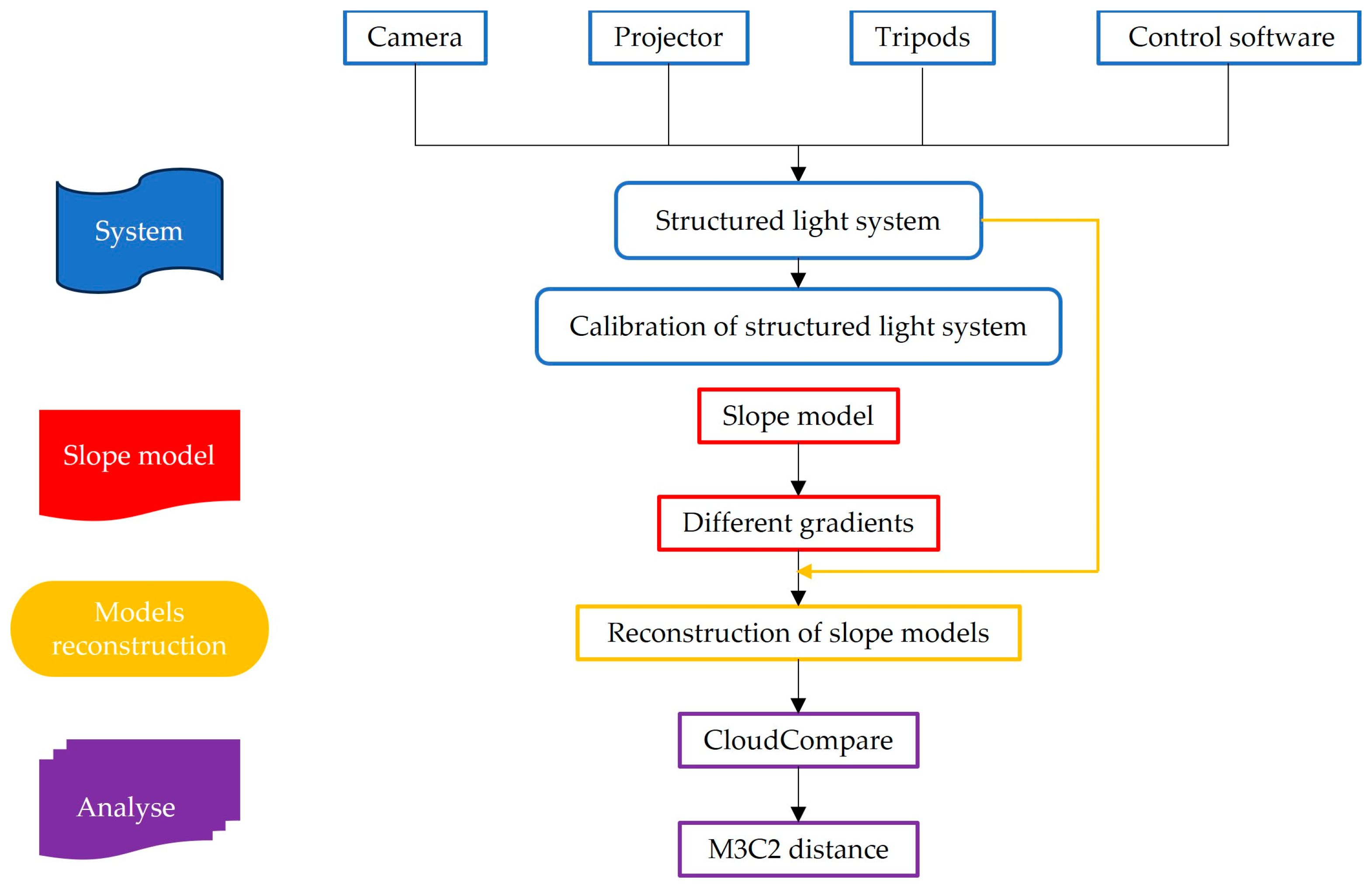
2. Structured Light System
2.1. Design of Gray Code Coding Pattern
2.2. Gray Code Decoding
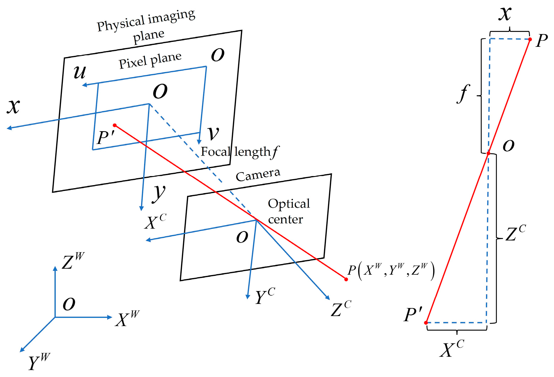
2.3. Calibration of Structured Light System
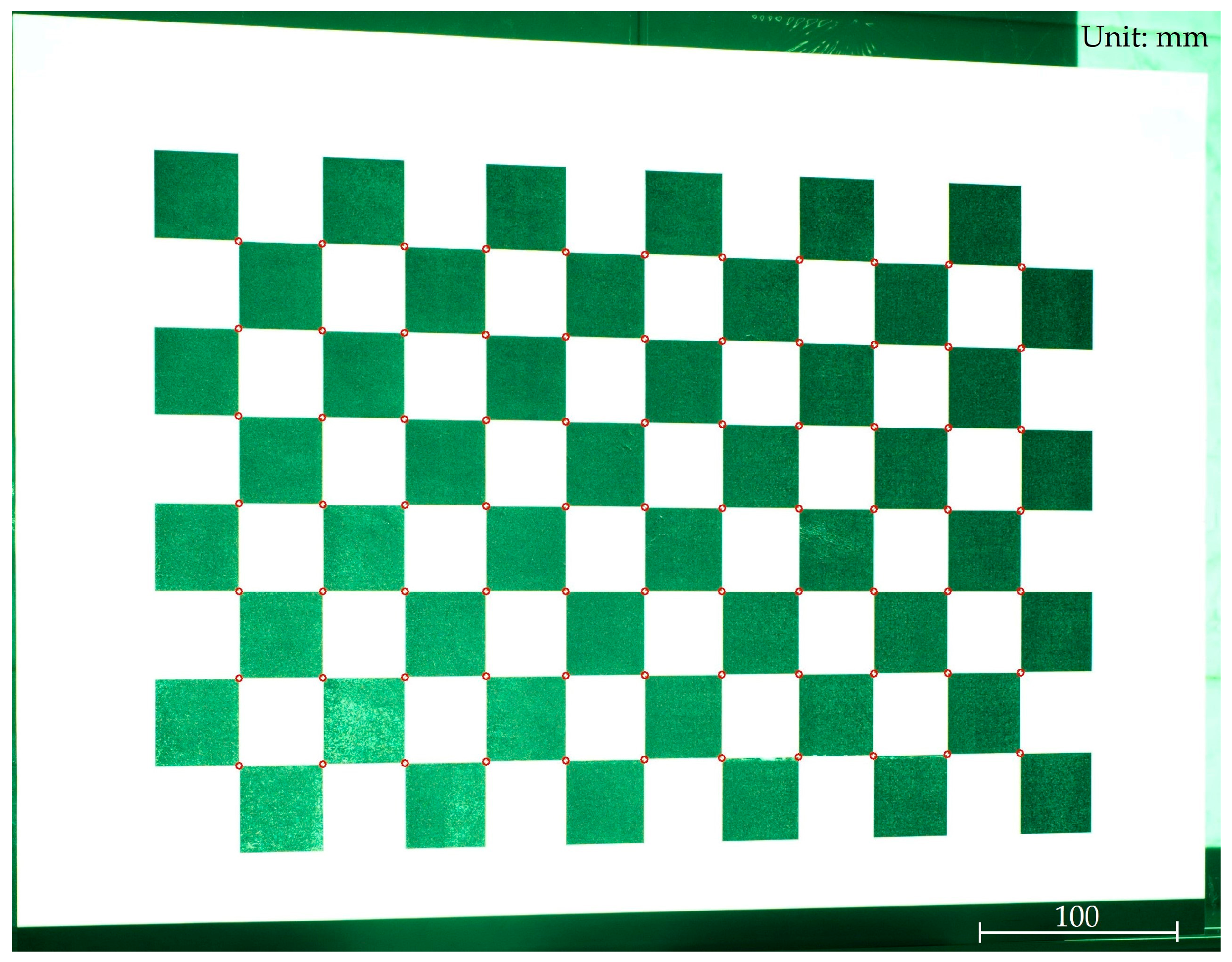
2.3.1. Calibration of the Camera
2.3.2. Calibration of the Projector
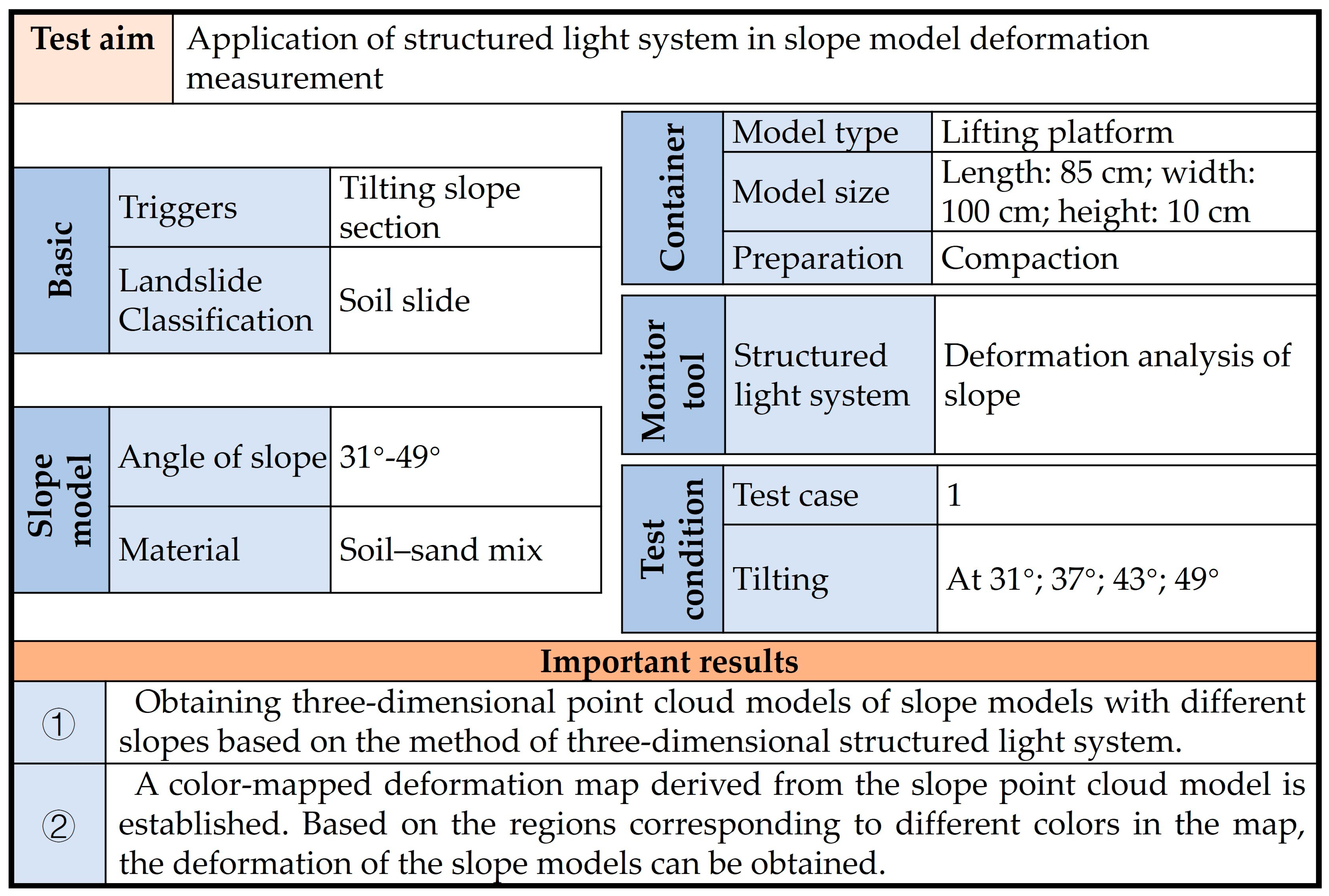
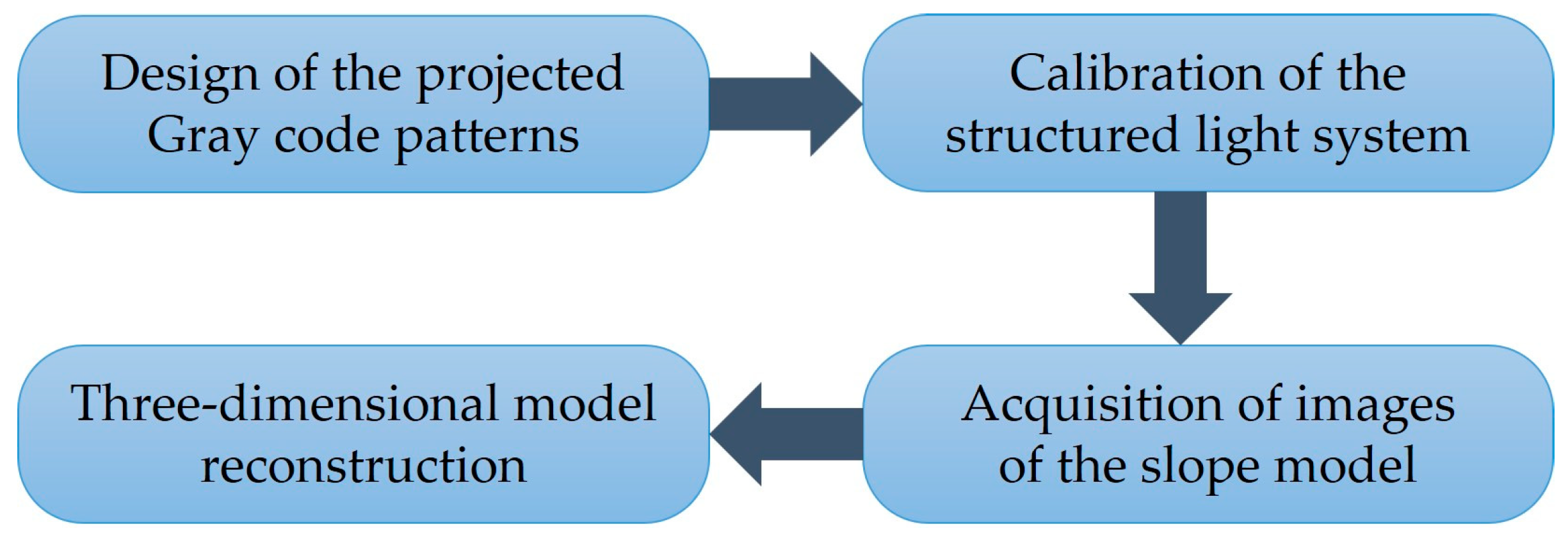
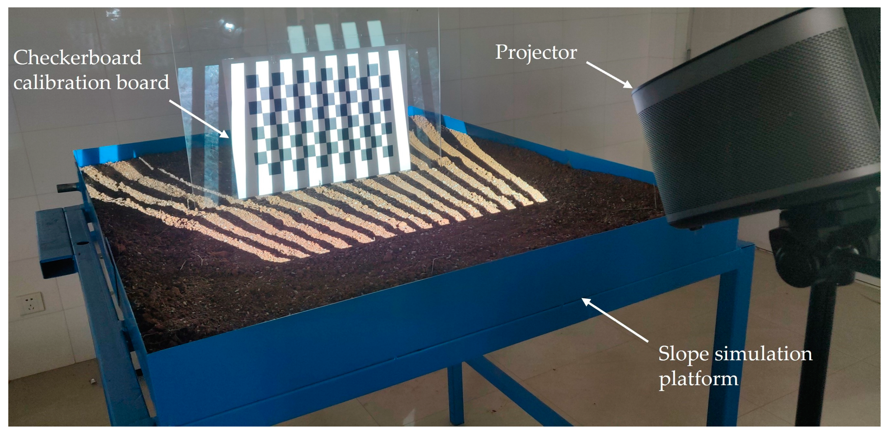
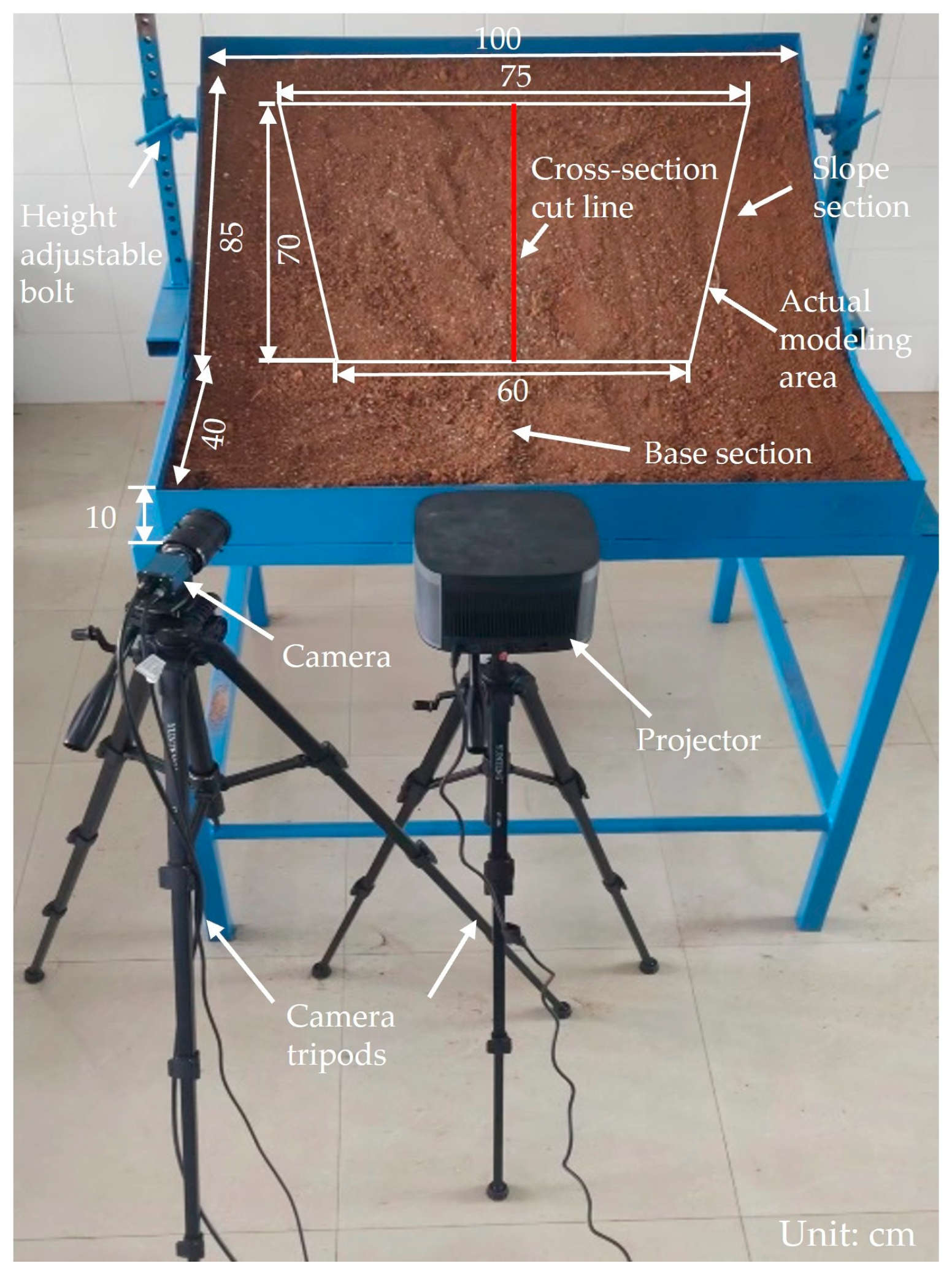
3. Three-Dimensional Modeling and Analysis for Slope Models
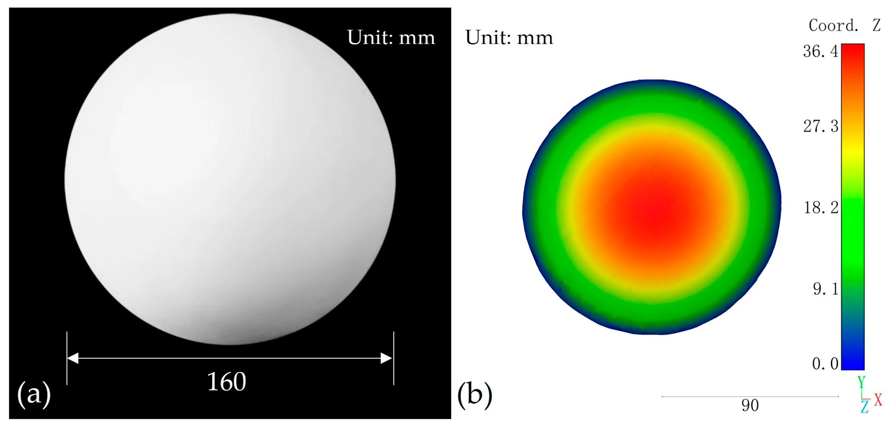
3.1. Accuracy Verification Experiment
3.2. Acquisition of Parameters for Structured Light System
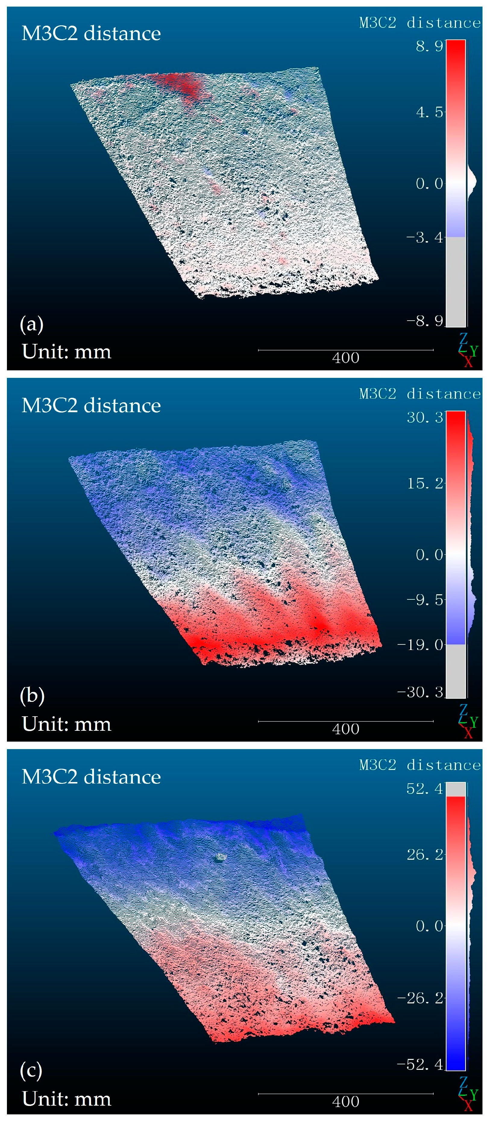
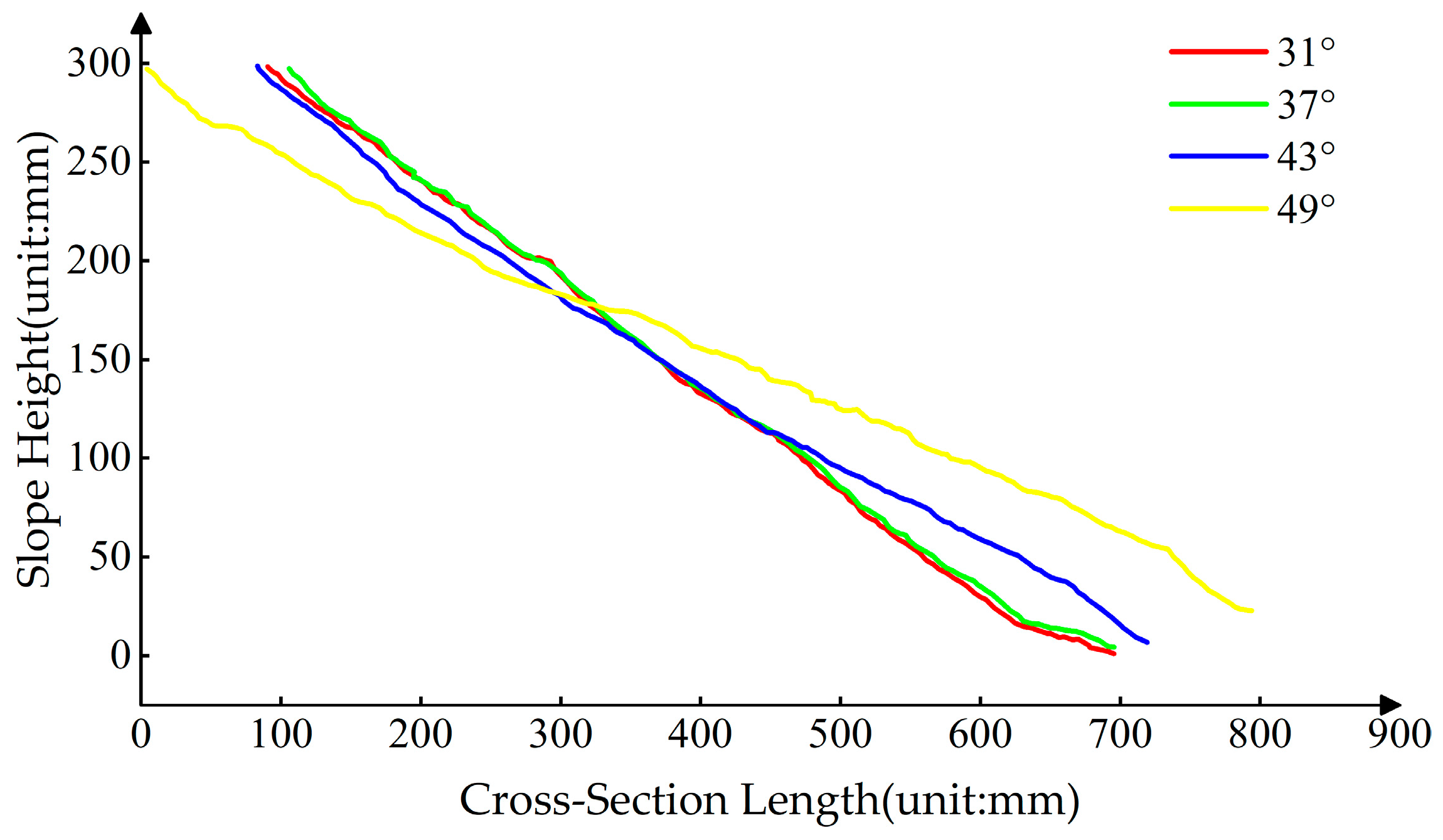
3.3. Simulation and Deformation Measurement of Slope Model Landslide Hazards
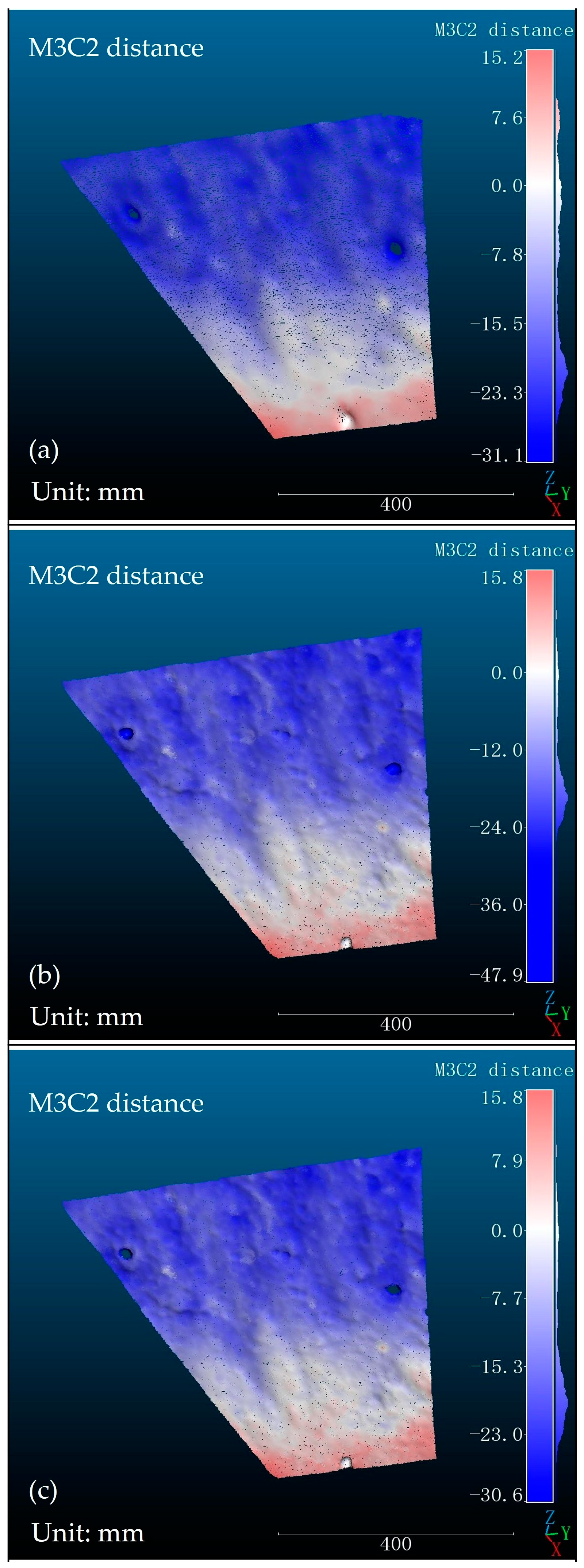
3.4. Comparison of the Landslide Prediction Method of Structured Light with the Landslide Prediction Method of the Laser
4. Discussion and Conclusions
Author Contributions
Funding
Institutional Review Board Statement
Informed Consent Statement
Data Availability Statement
Conflicts of Interest
Appendix A
References
- Osasan, K.S.; Afeni, T.B. Review of surface mine slope monitoring techniques. J. Min. Sci. 2010, 46, 177–186. [Google Scholar] [CrossRef]
- Ohnishi, Y.; Nishiyama, S.; Yano, T.; Matsuyama, H.; Amano, K. A study of the application of digital photogrammetry to slope monitoring systems. Int. J. Rock Mech. Min. Sci. 2006, 43, 756–766. [Google Scholar] [CrossRef]
- Guo, Z.; Zhou, M.; Huang, Y.; Pu, J.; Zhou, S.; Fu, B.; Aydin, A. Monitoring performance of slopes via ambient seismic noise recordings: Case study in a colluvium deposit. Eng. Geol. 2023, 324, 107268. [Google Scholar] [CrossRef]
- Take, W.A.; Bolton, M.D.; Wong, P.C.P.; Yeung, F.J. Evaluation of landslide triggering mechanisms in model fill slopes. Landslides 2004, 1, 173–184. [Google Scholar] [CrossRef]
- Wang, G.; Sassa, K. Pore-pressure generation and movement of rainfall-induced landslides: Effects of grain size and fine-particle content. Eng. Geol. 2003, 69, 109–125. [Google Scholar] [CrossRef]
- Zhu, C.; He, M.; Karakus, M.; Cui, X.; Tao, Z. Investigating toppling failure mechanism of anti-dip layered slope due to excavation by physical modelling. Rock Mech. Rock Eng. 2020, 53, 5029–5050. [Google Scholar] [CrossRef]
- Rouainia, M.; Davies, O.; O’Brien, T.; Glendinning, S. Numerical modelling of climate effects on slope stability. Proc. Inst. Civ. Eng.-Eng. Sustain. 2009, 162, 81–89. [Google Scholar] [CrossRef]
- Lee, L.M.; Kassim, A.; Gofar, N. Performances of two instrumented laboratory models for the study of rainfall infiltration into unsaturated soils. Eng. Geol. 2011, 117, 78–89. [Google Scholar] [CrossRef]
- Xu, J.; Ueda, K.; Uzuoka, R. Evaluation of failure of slopes with shaking-induced cracks in response to rainfall. Landslides 2022, 19, 119–136. [Google Scholar] [CrossRef]
- Zarrabi, M.; Eslami, A. Behavior of piles under different installation effects by physical modeling. Int. J. Geomech. 2016, 16, 04016014. [Google Scholar] [CrossRef]
- Ahmadi, M.; Moosavi, M.; Jafari, M.K. Experimental investigation of reverse fault rupture propagation through wet granular soil. Eng. Geol. 2018, 239, 229–240. [Google Scholar] [CrossRef]
- Zhang, B.; Fang, K.; Tang, H.; Sumi, S.; Ding, B. Block-flexure toppling in an anaclinal rock slope based on multi-field monitoring. Eng. Geol. 2023, 327, 107340. [Google Scholar] [CrossRef]
- Huang, C.C.; Lo, C.L.; Jang, J.S.; Hwu, L.K. Internal soil moisture response to rainfall-induced slope failures and debris discharge. Eng. Geol. 2008, 101, 134–145. [Google Scholar] [CrossRef]
- Hu, X.; Zhou, C.; Xu, C.; Liu, D.; Wu, S.; Li, L. Model tests of the response of landslide-stabilizing piles to piles with different stiffness. Landslides 2019, 16, 2187–2200. [Google Scholar] [CrossRef]
- Huang, Y.; Xu, X.; Liu, J.; Mao, W. Centrifuge modeling of seismic response and failure mode of a slope reinforced by a pile-anchor structure. Soil Dyn. Earthq. Eng. 2020, 131, 106037. [Google Scholar] [CrossRef]
- Pipatpongsa, T.; Fang, K.; Leelasukseree, C.; Chaiwan, A. Stability analysis of laterally confined slope lying on inclined bedding plane. Landslides 2022, 19, 1861–1879. [Google Scholar] [CrossRef]
- Yin, Y.; Deng, Q.; Li, W.; He, K.; Wang, Z.; Li, H.; An, P.; Fang, K. Insight into the crack characteristics and mechanisms of retrogressive slope failures: A large-scale model test. Eng. Geol. 2023, 327, 107360. [Google Scholar] [CrossRef]
- Wang, C.; Wang, H.; Qin, W.; Wei, S.; Tian, H.; Fang, K. Behaviour of pile-anchor reinforced landslides under varying water level, rainfall, and thrust load: Insight from physical modelling. Eng. Geol. 2023, 325, 107293. [Google Scholar] [CrossRef]
- Chang, Z.; Huang, F.; Huang, J.; Jiang, S.-H.; Zhou, C.; Zhu, L. Experimental study of the failure mode and mechanism of loess fill slopes induced by rainfall. Eng. Geol. 2021, 280, 105941. [Google Scholar] [CrossRef]
- Fang, K.; Miao, M.; Tang, H.; Jia, S.; Dong, A.; An, P.; Zhang, B. Insights into the deformation and failure characteristic of a slope due to excavation through multi-field monitoring: A model test. Acta Geotech. 2023, 18, 1001–1024. [Google Scholar] [CrossRef]
- Baba, H.O.; Peth, S. Large scale soil box test to investigate soil deformation and creep movement on slopes by Particle Image Velocimetry (PIV). Soil Tillage Res. 2012, 125, 38–43. [Google Scholar] [CrossRef]
- Sarkhani Benemaran, R.; Esmaeili-Falak, M.; Katebi, H. Physical and numerical modelling of pile-stabilised saturated layered slopes. Proc. Inst. Civ. Eng.-Geotech. Eng. 2022, 175, 523–538. [Google Scholar]
- Zhang, D.; Zhang, Y.; Cheng, T.; Meng, Y.; Fang, K.; Garg, A.; Garg, A. Measurement of displacement for open pit to underground mining transition using digital photogrammetry. Measurement 2017, 109, 187–199. [Google Scholar] [CrossRef]
- Liu, D.; Hu, X.; Zhou, C.; Xu, C.; He, C.; Zhang, H.; Wang, Q. Deformation mechanisms and evolution of a pile-reinforced landslide under long-term reservoir operation. Eng. Geol. 2020, 275, 105747. [Google Scholar] [CrossRef]
- Abellán, A.; Oppikofer, T.; Jaboyedoff, M.; Rosser, N.J.; Lim, M.; Lato, M.J. Terrestrial laser scanning of rock slope instabilities. Earth Surf. Process. Landf. 2014, 39, 80–97. [Google Scholar] [CrossRef]
- Francioni, M.; Salvini, R.; Stead, D.; Coggan, J. Improvements in the integration of remote sensing and rock slope modelling. Nat. Hazards 2018, 90, 975–1004. [Google Scholar] [CrossRef]
- Huo, G.; Wu, Z.; Li, J.; Li, S. Underwater target detection and 3D reconstruction system based on binocular vision. Sensors 2018, 18, 3570. [Google Scholar] [CrossRef]
- Tian, X.; Liu, R.; Wang, Z.; Ma, J. High quality 3D reconstruction based on fusion of polarization imaging and binocular stereo vision. Inf. Fusion 2022, 77, 19–28. [Google Scholar] [CrossRef]
- Woodham, R.J. Photometric method for determining surface orientation from multiple images. Opt. Eng. 1980, 19, 139–144. [Google Scholar] [CrossRef]
- Barsky, S.; Petrou, M. The 4-source photometric stereo technique for three-dimensional surfaces in the presence of highlights and shadows. IEEE Trans. Pattern Anal. Mach. Intell. 2003, 25, 1239–1252. [Google Scholar] [CrossRef]
- Zhou, P.; Zhu, J.; Jing, H. Optical 3-D surface reconstruction with color binary speckle pattern encoding. Opt. Express 2018, 26, 3452–3465. [Google Scholar] [CrossRef] [PubMed]
- Zhang, Q.; Xu, R.; Liu, Y.; Chen, Z. 3D shape measurement based on digital speckle projection and spatio-temporal correlation. Proceedings 2018, 2, 552. [Google Scholar]
- Yin, X.; Wang, G.; Shi, C.; Liao, Q. Efficient active depth sensing by laser speckle projection system. Opt. Eng. 2014, 53, 013105. [Google Scholar] [CrossRef]
- Jiang, J.; Cheng, J.; Zhao, H. Stereo matching based on random speckle projection for dynamic 3D sensing. In Proceedings of the 2012 11th International Conference on Machine Learning and Applications, Boca Raton, FL, USA, 12–15 December 2012; Volume 1, pp. 191–196. [Google Scholar]
- Gühring, J. Dense 3D surface acquisition by structured light using off-the-shelf components. In Proceedings of the Videometrics and Optical Methods for 3D Shape Measurement, San Jose, CA, USA, 22 December 2000; Volume 4309, pp. 220–231. [Google Scholar]
- Ettl, S.; Arold, O.; Yang, Z.; Häusler, G. Flying triangulation—An optical 3D sensor for the motion-robust acquisition of complex objects. Appl. Opt. 2012, 51, 281–289. [Google Scholar] [CrossRef] [PubMed]
- Sato, K. Range-image system utilizing nematic liquid crystal mask. In Proceedings of the 1st International Conference on Computer Vision (ICCV), London, UK, 8–11 June 1987; pp. 657–661. [Google Scholar]
- Ishii, I.; Yamamoto, K.; Doi, K.; Tsuji, T. High-speed 3D image acquisition using coded structured light projection. In Proceedings of the 2007 IEEE/RSJ International Conference on Intelligent Robots and Systems, San Diego, CA, USA, 29 October–2 November 2007; pp. 925–930. [Google Scholar]
- Valkenburg, R.J.; McIvor, A.M. Accurate 3D measurement using a structured light system. Image Vis. Comput. 1998, 16, 99–110. [Google Scholar] [CrossRef]
- Su, X.; Chen, W. Fourier transform profilometry: A review. Opt. Lasers Eng. 2001, 35, 263–284. [Google Scholar] [CrossRef]
- Kemao, Q. Windowed Fourier transform for fringe pattern analysis. Appl. Opt. 2004, 43, 2695–2702. [Google Scholar] [CrossRef]
- Zuo, C.; Feng, S.; Huang, L.; Tao, T.; Yin, W.; Chen, Q. Phase shifting algorithms for fringe projection profilometry: A review. Opt. Lasers Eng. 2018, 109, 23–59. [Google Scholar] [CrossRef]
- Zhang, Y.; Xiong, Z.; Wu, F. Unambiguous 3D measurement from speckle-embedded fringe. Appl. Opt. 2013, 52, 7797–7805. [Google Scholar] [CrossRef]
- Ren, M.; Wang, X.; Xiao, G.; Chen, M.; Fu, L. Fast defect inspection based on data-driven photometric stereo. IEEE Trans. Instrum. Meas. 2018, 68, 1148–1156. [Google Scholar] [CrossRef]
- Ju, Y.; Jian, M.; Wang, C.; Zhang, C.; Dong, J.; Lam, K.-M. Estimating high-resolution surface normals via low-resolution photometric stereo images. IEEE Trans. Circuits Syst. Video Technol. 2023. early access. [Google Scholar] [CrossRef]
- Chen, G.; Han, K.; Wong, K.Y.K. PS-FCN: A flexible learning framework for photometric stereo. In Proceedings of the European Conference on Computer Vision (ECCV), Munich, Germany, 8–14 September 2018; pp. 3–18. [Google Scholar]
- Trobina, M. Error Model of a Coded-Light Range Sensor; Technique Report; Communication Technology Laboratory, ETH Zentrum: Zurich, Switzerland, 1995. [Google Scholar]
- Inokuchi, S. Range imaging system for 3-D object recognition. In Proceedings of the International Conference on Pattern Recognition (ICPR), Montreal, QC, Canada, 30 July–2 August 1984. [Google Scholar]
- Nie, L.; Ye, Y.; Song, Z. Method for calibration accuracy improvement of projector-camera-based structured light system. Opt. Eng. 2017, 56, 074101. [Google Scholar] [CrossRef]
- Chen, C.; Gao, N.; Zhang, Z. Simple calibration method for dual-camera structured light system. J. Eur. Opt. Soc.-Rapid Publ. 2018, 14, 23. [Google Scholar] [CrossRef]
- Hartley, R.; Zisserman, A. Multiple View Geometry in Computer Vision; Cambridge University Press: Cambridge, UK, 2003. [Google Scholar]
- Yilmaz, Ö.; Karakuş, F. Stereo and KinectFusion for continuous 3D reconstruction and visual odometry. Turk. J. Electr. Eng. Comput. Sci. 2016, 24, 2756–2770. [Google Scholar] [CrossRef]
- Zhang, Z. A flexible new technique for camera calibration. IEEE Trans. Pattern Anal. Mach. Intell. 2000, 22, 1330–1334. [Google Scholar] [CrossRef]
- Falcao, G.; Hurtos, N.; Massich, J. Plane-based calibration of a projector-camera system. VIBOT Master 2008, 9, 1–12. [Google Scholar]
- Zhang, S.; Huang, P.S. Novel method for structured light system calibration. Opt. Eng. 2006, 45, 083601. [Google Scholar]
- Moreno, D.; Taubin, G. Simple, accurate, and robust projector-camera calibration. In Proceedings of the 2012 Second International Conference on 3D Imaging, Modeling, Processing, Visualization & Transmission, Zurich, Switzerland, 13–15 October 2012; pp. 464–471. [Google Scholar]
- Fang, K.; Tang, H.; Li, C.; Su, X.; An, P.; Sun, S. Centrifuge modelling of landslides and landslide hazard mitigation: A review. Geosci. Front. 2023, 14, 101493. [Google Scholar] [CrossRef]
- Bell, T.; Li, B.; Zhang, S. Structured light techniques and applications. In Wiley Encyclopedia of Electrical and Electronics Engineering; John Wiley & Sons, Inc.: Hoboken, NJ, USA, 1999; pp. 1–24. [Google Scholar]
- Zhang, S. High-speed 3D shape measurement with structured light methods: A review. Opt. Lasers Eng. 2018, 106, 119–131. [Google Scholar] [CrossRef]
- Fofi, D.; Sliwa, T.; Voisin, Y. A comparative survey on invisible structured light. In Proceedings of the Machine Vision Applications in Industrial Inspection XII, San Jose, CA, USA, 3 May 2004; Volume 5303, pp. 90–98. [Google Scholar]
- Schaffer, M.; Große, M.; Harendt, B.; Kowarschik, R. Outdoor three-dimensional shape measurements using laser-based structured illumination. Opt. Eng. 2012, 51, 090503. [Google Scholar] [CrossRef]


| Manufacturer | Model | Standard Resolution | Luminance | Contrast |
|---|---|---|---|---|
| XGIMI (Beijing, China) | H3S | 1920 × 1080 | 2200ANSI lm | 1000:1 |
| Manufacturer | Model | Sensor Type | Sensor Size | Image Format | Focal Length | Aperture |
|---|---|---|---|---|---|---|
| DAHENG (Beijing, China) | HF2514V-2 | CCD | 1.1 in. | 4096 × 3000 | 25 mm | f/1.4 |
| Type | Evaluation Metrics | Calculation Result |
|---|---|---|
| Sphere (r = 80) | Fit Radius | 80.13 |
| Absolute Error | 0.13 | |
| RMSE | 0.22 |
| Manufacturer | Model | Dimensions | Scanning Area | Accuracy | Scan Speed | Working Distance |
|---|---|---|---|---|---|---|
| XIANLIN (Hangzhou, China) | FreeScan Combo | 193 × 63 × 53 mm | 1000 × 800 mm | 0.02 mm | 3,500,000 scan/s | 300 mm |
| Type | 99% | RMSE |
|---|---|---|
| M3C2 | 3.61 mm | 1.08 |
| Hardware Type | Parameter Type | Parametric Expression | Calibration Result |
|---|---|---|---|
| Camera | Internal reference matrix | ||
| Aberration coefficient | |||
| Projector | Internal reference matrix | ||
| Aberration coefficient | |||
| Structured Light System | Rotation matrix | ||
| Translation vector |
Disclaimer/Publisher’s Note: The statements, opinions and data contained in all publications are solely those of the individual author(s) and contributor(s) and not of MDPI and/or the editor(s). MDPI and/or the editor(s) disclaim responsibility for any injury to people or property resulting from any ideas, methods, instructions or products referred to in the content. |
© 2024 by the authors. Licensee MDPI, Basel, Switzerland. This article is an open access article distributed under the terms and conditions of the Creative Commons Attribution (CC BY) license (https://creativecommons.org/licenses/by/4.0/).
Share and Cite
Chen, Z.; Zhang, C.; Tang, Z.; Fang, K.; Xu, W. Three-Dimensional Reconstruction and Deformation Identification of Slope Models Based on Structured Light Method. Sensors 2024, 24, 794. https://doi.org/10.3390/s24030794
Chen Z, Zhang C, Tang Z, Fang K, Xu W. Three-Dimensional Reconstruction and Deformation Identification of Slope Models Based on Structured Light Method. Sensors. 2024; 24(3):794. https://doi.org/10.3390/s24030794
Chicago/Turabian StyleChen, Zhijian, Changxing Zhang, Zhiyi Tang, Kun Fang, and Wei Xu. 2024. "Three-Dimensional Reconstruction and Deformation Identification of Slope Models Based on Structured Light Method" Sensors 24, no. 3: 794. https://doi.org/10.3390/s24030794
APA StyleChen, Z., Zhang, C., Tang, Z., Fang, K., & Xu, W. (2024). Three-Dimensional Reconstruction and Deformation Identification of Slope Models Based on Structured Light Method. Sensors, 24(3), 794. https://doi.org/10.3390/s24030794