
Application of Machine Learning to Predict CO2 Emissions in Light-Duty Vehicles


Abstract
:1. Introduction
1.1. Research Objectives
- i.
- An exploration of the ideas and conceptual framework of digital transformation in transportation, and the impact on GHG emissions.
- ii.
- The identification of significant features influencing vehicular CO2 emissions.
- iii.
- The development and evaluation of an ML model for predicting CO2 emissions in light-duty vehicles.
- iv.
- The deployment of a web-based application as a practical tool for stakeholders to estimate the CO2 emitted by a vehicle.
1.2. Problem Statement
1.3. Research Scope
2. Literature Review
2.1. The Concept of Digital Transformation
2.2. Emerging Technologies and Their Contribution to Transformation in Transportation
2.2.1. Internet of Things (IoT) in Transportation
2.2.2. Artificial Intelligence (AI) in Transportation
2.2.3. Intelligent Transportation Systems (ITSs)
2.3. Sensor-Based Emission Measurement Systems
2.4. Machine Learning Models for Calculating CO2 Emissions in Cars
3. Methodology
3.1. Quantitative and Predictive Analysis
3.2. Dataset Selection
- i.
- Manufacturer, model, description, etc.: minor missing values, around 0.2%.
- ii.
- Transmission: about 3.66% missing.
- iii.
- Engine power (Kw/PS): missing values range from about 1.19% to 1.86%.
- iv.
- Electric energy consumption Miles/kWh, wh/km, maximum range (Km/Miles), etc.: high percentage of missing values, exceeding 50%.
- v.
- WLTP metrics: varies significantly, with some columns having a small percentage of missing values and others having more.
- vi.
- Annual costs, noise level, emissions data: varying degrees of missing data, with some columns missing over 50% of their values.
3.3. Data Cleaning
3.4. Data Exploration and Pre-Processing
3.4.1. Descriptive Categorical and Statistical Analysis
3.4.2. Managing Outliers
3.4.3. Correlation
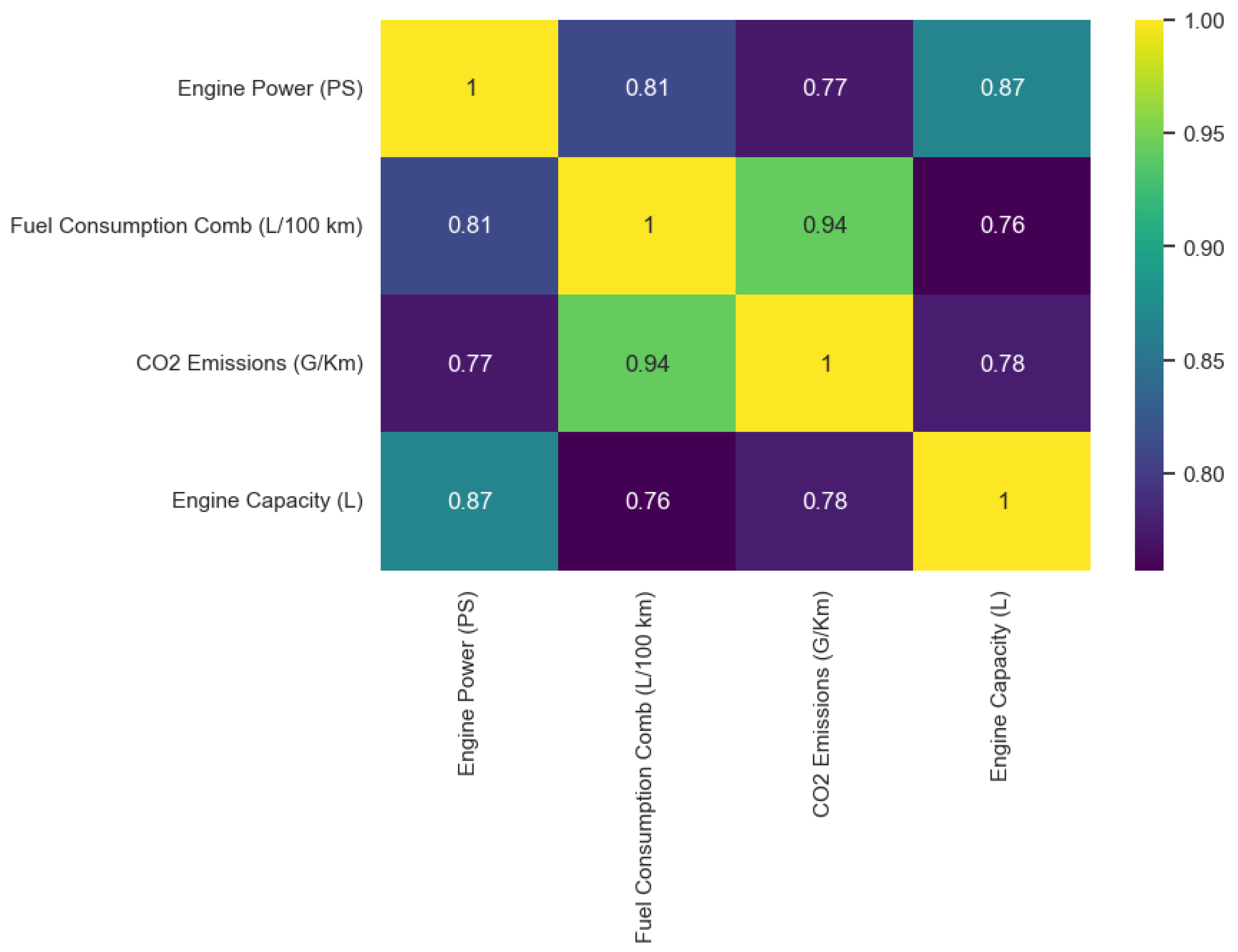
Insights from the Correlation
- The correlation between engine power (PS) and fuel consumption comb (L/100 km) is 0.81, indicating that there is a very strong positive correlation between the variables. So, an increase in the engine power of a vehicle will increase the quantity of fuel consumed by the vehicle.
- The correlation between engine power (PS) and CO2 emissions (G/Km) is strong at 0.77, meaning CO2 emissions are likely to be low in vehicles with low engine power (PS).
- There is a 0.87 correlation between engine power (PS) and engine capacity (L), meaning a car with a large engine size will be more powerful than a car with a smaller engine capacity.
- There is a very high positive correlation (0.94) between fuel consumption comb (L/100 km) and CO2 emissions (G/km), meaning the more fuel a vehicle consumes, the more CO2 emissions it produces.
- The relationship between fuel consumption comb (L/100 km) and engine capacity (L) has a correlation coefficient of 0.76, so it is a strong positive relationship.
- Similarly, the correlation between CO2 emissions (G/Km) and engine capacity (L) is a little below average at 0.78. This indicates a strong positive relationship between the variables.
3.5. Building the Machine Learning Model
3.5.1. Cleaned Dataset Variables
- i.
- Numerical Variables:
- Target variable: CO2 emissions (g/km)—This variable represents the grams of CO2 emitted per kilometer driven. It is the variable we aim to predict.
- Engine power (PS): This variable is directly related to fuel consumption and CO2 emissions. Higher power generally implies higher fuel consumption and emissions.
- Fuel consumption comb (L/100 km): Combined fuel consumption liters per 100 km. This is a highly relevant and strongly correlated predictor of CO2 emissions.
- Engine capacity (L): Engine displacement in liters. A larger engine capacity often, but not always, correlates with higher power and fuel consumption.
- ii.
- Categorical Variables:
- Manufacturer: The brand of the vehicle. This is a high-cardinality categorical variable with numerous unique values (initially 40).
- Model: The specific model of the vehicle. This is a very high-cardinality categorical variable (initially 656 unique values).
- Transmission: Describes the type of transmission (e.g., manual, automatic, CVT). It is a moderately high-cardinality categorical variable (initially 54 unique values), with some ambiguity in naming conventions.
- Fuel type: Indicates the type of fuel used (e.g., petrol, diesel, petrol electric). This is a low-cardinality categorical variable (initially 7 unique values) with significant influence on CO2 emissions.
- Powertrain: Specifies the powertrain configuration (e.g., Internal Combustion Engine (ICE) or Hybrid Electric Vehicle (HEV)). This low-cardinality categorical variable (initially 5 unique values) is a strong predictor, as different powertrain types vary considerably in their fuel efficiency.
3.5.2. Feature Selection Process
- i.
- Initial Feature Elimination: The high-cardinality features manufacturer and model were removed. Including these features would lead to a very high-dimensional feature space after one-hot encoding, increasing computational complexity and significantly increasing the risk of overfitting. The impact of these features may be implicitly captured by other features (e.g., engine type and fuel efficiency). This step is a common practice when dealing with high-cardinality categorical predictors in regression tasks.
- ii.
- Pre-processing of Remaining Categorical Features: The remaining categorical features (transmission, fuel type, powertrain) were pre-processed to ensure consistency. This involved replacing spaces and hyphens with underscores (“_”) to standardize the categorical variable labels, preventing issues caused by inconsistent representations. This is standard practice to improve model performance with categorical data.
- iii.
- One-Hot Encoding: One-hot encoding was applied to the pre-processed categorical variables to transform them into numerical representations suitable for model training. This is a widely used and effective method for encoding categorical data in machine learning.
- iv.
- Standardization of Numerical Features: The continuous features (engine power (PS), fuel consumption comb (L/100 km), engine capacity (L)) were standardized to ensure they have zero mean and unit variance. This helps prevent features with larger scales from dominating the model and improves the performance of some algorithms like linear regression.
- v.
- Outlier Removal: Exploratory data analysis using scatter plots revealed outliers, primarily in the relationship between fuel consumption and CO2 emissions, indicating potential data errors. These outliers were removed. This step is crucial because outliers can disproportionately affect the performance of some regression models, particularly linear ones.
3.5.3. Regression Analysis
- I.
- Linear regression: Linear regression is applicable when the dependent variables and the variable to be predicted are in a linear relationship. The most popular types of linear regression are simple linear regression and multiple linear regression [82]. Linear regression models can be quickly trained, are easy to understand, and have a stable performance compared to other algorithms [83].where y is the dependent value to be predicted, x is the independent value, and w is the intercepted values when the value of y and x is zero.
- II.
- Random Forest regression: This is a machine learning algorithm that uses the ensemble method to group and use the decisions from multiple models to accurately make a prediction [84].where g is the final predicted model, and etc., are the base models.
3.6. Performance Parameters
3.6.1. Mean Squared Error
3.6.2. Root Mean Squared Error
3.6.3. Mean Absolute Error (MAE)
3.6.4. Mean Absolute Percentage Error (MAPE)
4. Results and Discussion
4.1. Comparative Analysis of the Regression Models
- i.
- Random Forest Regressor:Random Forest is an ensemble method that is less prone to overfitting due to its ability to handle both categorical and numerical features directly.
- Performance: In this research, the Random Forest Regressor demonstrated excellent performance, achieving a low MAE (2.33), RMSE (6.67), and MAPE (1.81%). This suggests high accuracy and relatively small prediction errors.
- Strengths: Handles non-linear relationships effectively, is less prone to overfitting than individual Decision Trees, is relatively insensitive to outliers, and can manage high-dimensional data.
- Weaknesses: The model can be a “black box”, making interpretation difficult.
- ii.
- Linear Regression:Linear regression models the relationship between a dependent variable (CO2 emissions) and one or more independent variables (features) as a linear equation.
- Performance: Linear regression exhibited a comparatively higher MAE (3.61), RMSE (7.48), and MAPE (2.73%). This indicates lower accuracy than the ensemble methods.
- Strengths: Simple to understand and interpret.
- Weaknesses: Assumes a linear relationship, highly sensitive to outliers, performs poorly with non-linear relationships, and requires careful feature scaling (handled here by StandardScaler during modeling).
- iii.
- Decision Tree Regressor:Decision Tree Regression builds a tree-like model where each branch represents a feature, each node represents a decision based on a feature value, and each leaf node represents a predicted value.
- Performance: Surprisingly, the Decision Tree Regressor achieved the lowest MAE (2.20) and MAPE (1.69%) among all the models. This indicates high accuracy, but the RMSE (7.26) was higher, suggesting some outliers had a bigger impact on the MSE.
- Strengths: Simple to interpret, handles both categorical and numerical features well, and can capture non-linear relationships.
- Weaknesses: Highly prone to overfitting, and sensitive to small changes in the training data. The low MAE/MAPE and high RMSE suggest potential overfitting.
- iv.
- Gradient Boosting Regressor:Gradient Boosting is another ensemble method that sequentially builds trees, where each subsequent tree corrects the errors made by its predecessors.
- Performance: Gradient Boosting showed good performance in terms of the MAE (3.13), RMSE (6.37), and MAPE (2.27%). The RMSE was slightly lower than that of Random Forest, suggesting it may be a bit more robust to outliers in this dataset.
- Strengths: High accuracy, handles non-linear relationships effectively, and less prone to overfitting than a single Decision Tree.
- Weaknesses: The model is more complex to interpret than linear regression.
- v.
- Lasso Regression:Lasso Regression is a linear model that incorporates L1 regularization to shrink coefficients towards zero, effectively performing feature selection and reducing overfitting. The alpha parameter controls the strength of regularization.
- Performance: Lasso Regression demonstrated the highest MAE (4.54) and RMSE (9.06) and a relatively high MAPE (3.41%). This suggests its performance was inferior to other models, likely due to the alpha value chosen and the non-linear nature of the data.
- Strengths: Reduces overfitting and performs feature selection.
- Weaknesses: Sensitive to outliers, assumes a linear relationship. The choice of alpha is crucial and requires careful tuning using techniques such as cross-validation.
- vi.
- Ridge Regression:Similarly to Lasso, Ridge Regression is a linear model that uses L2 regularization to constrain coefficient magnitudes. It does not perform feature selection as aggressively as Lasso.
- Performance: Ridge Regression performed similarly to linear regression, with a relatively high MAE (7.48), RMSE (7.48), and MAPE (2.73%), indicating less predictive power compared to the tree-based and ensemble models.
- Strengths: Reduces overfitting and handles multicollinearity better than linear regression.
- Weaknesses: Assumes a linear relationship and does not perform feature selection.
4.2. Deployment to Streamlit
5. Conclusions
Limitations and Future Work
Author Contributions
Funding
Institutional Review Board Statement
Informed Consent Statement
Data Availability Statement
Conflicts of Interest
Appendix A


| Features of the Datasets |
|---|
| Manufacturer: The company that manufactures the vehicle. Model: The specific model of the vehicle. Description: A detailed description of the vehicle, possibly including sub-model or variant. Transmission: The type of transmission used in the vehicle (e.g., automatic or manual). Engine capacity: The size of the engine in the vehicle, typically measured in cubic centimeters (cc) or liters. Fuel type: The type of fuel the vehicle uses (e.g., petrol, diesel, electricity/petrol). Powertrain: The mechanism by which power is transmitted from the engine to the wheels of the vehicle. (e.g., Internal Combustion Engine (ICE), Hybrid Electric Vehicle (HEV), Plug-in Hybrid Electric Vehicle (PHEV)) Engine power (Kw): The power output of the engine in kilowatts. Engine power (PS): The power output of the engine in metric horsepower (PS). Testing scheme: The protocol under which the vehicle was tested (e.g., WLTP—Worldwide Harmonised Light Vehicle Test Procedure). Euro standard: The European emission standard the vehicle conforms to. The Euro standard for the datasets is Euro 6. Diesel VED supplement: Indicates whether the vehicle is subject to the Diesel Vehicle Excise Duty supplement. Electric energy consumption Miles/kWh: The vehicle’s energy efficiency in miles per kilowatt-hour. Wh/km: Energy consumption in watt-hours per kilometer. Maximum range (km): The maximum distance the vehicle can travel on a single charge or full tank in kilometers. Maximum range (miles): The maximum distance the vehicle can travel on a single charge or full tank in miles. WLTP imperial low/medium/high/extra high/combined: Fuel economy metrics under different WLTP conditions (low, medium, high, extra high, and combined) measured in miles per gallon (MPG). WLTP metric low/medium/high/extra high/combined: Fuel economy metrics under different WLTP conditions (low, medium, high, extra high, and combined) measured in liters per 100 km. WLTP CO2: Carbon dioxide emissions under the WLTP test cycle, measured in grams per kilometer. Equivalent all-electric range Miles/km: The range of the vehicle when operating in all-electric mode, measured in miles and kilometers. Electric range city Miles/km: The electric range of the vehicle in urban settings, in miles and kilometers. Annual fuel cost 10,000 miles: The estimated annual fuel cost for 10,000 miles. Annual electricity cost/10,000 miles: The estimated annual electricity cost for 10,000 miles. Total cost/10,000 miles: The total estimated cost (fuel or electricity) for 10,000 miles. Noise level dB(A): The noise level of the vehicle in decibels. Emissions CO [mg/km]: Carbon monoxide emissions in milligrams per kilometer. THC emissions [mg/km]: Total hydrocarbon emissions in milligrams per kilometer. Emissions NOx [mg/km]: Nitrogen oxide emissions in milligrams per kilometer. THC + NOx emissions [mg/km]: Combined total hydrocarbon and nitrogen oxide emissions in milligrams per kilometer. Particulates [No.] [mg/km]: The number of particulate matter emissions in milligrams per kilometer. RDE NOx urban/combined: Real driving emissions of nitrogen oxides in urban and combined conditions. |


References
- Abbass, K.; Qasim, M.Z.; Song, H.; Murshed, M.; Mahmood, H.; Younis, I. A Review of the Global Climate Change Impacts, Adaptation, and Sustainable Mitigation Measures. Environ. Sci. Pollut. Res. 2022, 29, 42539–42559. [Google Scholar] [CrossRef] [PubMed]
- Wang, F.; Harindintwali, J.D.; Yuan, Z.; Wang, M.; Wang, F.; Li, S.; Yin, Z.; Huang, L.; Fu, Y.; Li, L.; et al. Technologies and Perspectives for Achieving Carbon Neutrality. Innovation 2021, 2, 100180. [Google Scholar] [CrossRef] [PubMed]
- BEIS. 2021 UK Greenhouse Gas Emissions, Final Figures; National Statistics: London, UK, 2023. Available online: https://assets.publishing.service.gov.uk/media/63e131dde90e07626846bdf9/greenhouse-gas-emissions-statistical-release-2021.pdf (accessed on 18 October 2024).
- Lange, S.; Pohl, J.; Santarius, T. Digitalization and Energy Consumption. Does ICT Reduce Energy Demand? Ecol. Econ. 2020, 176, 106760. [Google Scholar] [CrossRef]
- Huang, Y.; Hu, M.; Xu, J.; Jin, Z. Digital Transformation and Carbon Intensity Reduction in Transportation Industry: Empirical Evidence from a Global Perspective. J. Environ. Manag. 2023, 344, 118541. [Google Scholar] [CrossRef] [PubMed]
- Li, F.; Trappey, A.J.C.; Lee, C.-H.; Li, L. Immersive Technology-Enabled Digital Transformation in Transportation Fields: A Literature Overview. Expert Syst. Appl. 2022, 202, 117459. [Google Scholar] [CrossRef]
- UNECE. Technical Report on the Development of a Worldwide Harmonised Light Duty Driving Test Procedure (WLTP). Available online: https://unece.org/fileadmin/DAM/trans/doc/2015/wp29grpe/GRPE-72-02.pdf (accessed on 18 October 2024).
- Intergovernmental Panel on Climate Change (IPCC). Summary for Policymakers. In Climate Change 2013: The Physical Science Basis; Contribution of Working Group I to the Fifth Assessment Report of the IPCC; Stocker, T.F., Qin, D., Plattner, G.-K., Tignor, M., Allen, S.K., Boschung, J., Eds.; Cambridge University Press: Cambridge, UK, 2013; pp. 1–30. [Google Scholar]
- Crippa, M.; Guizzardi, D.; Banja, M.; Solazzo, E.; Muntean, M.; Schaaf, E.; Pagani, F.; Monforti-Ferrario, F.; Olivier, J.; Quadrelli, R.; et al. CO2 Emissions of All World Countries—JRC/IEA/PBL 2022 Report; Publications Office of the European Union: Luxembourg, 2022. [Google Scholar] [CrossRef]
- EPA. Global Greenhouse Gas Emissions Data; US Environmental Protection Agency: Washington, DC, USA, 2022. Available online: https://www.epa.gov/ghgemissions/global-greenhouse-gas-emissions-data (accessed on 18 October 2024).
- Hayes, A. Transportation Sector; Investopedia: New York, NY, USA, 2021; Available online: https://www.investopedia.com/terms/t/transportation_sector.asp (accessed on 18 October 2024).
- UNEP. Transport; UNEP—UN Environment Programme: Nairobi, Kenya, 2017; Available online: https://www.unep.org/explore-topics/energy/what-we-do/transport (accessed on 18 October 2024).
- International Energy Agency. Transport—Energy System; IEA: Paris, France, 2023; Available online: https://www.iea.org/energy-system/transport (accessed on 18 October 2024).
- Westerman, G.; Bonnet, D.; McAfee, A. Leading Digital: Turning Technology into Business Transformation; Harvard Business Review Press: Boston, MA, USA, 2014. [Google Scholar]
- Ross, J.W.; Sebastian, I.M.; Beath, C.M. Designed for Digital: How to Architect Your Business for Sustained Success; MIT Press: Cambridge, MA, USA, 2019. [Google Scholar]
- Zhao, Y.; Li, X.; Wang, W.; Dai, P.; Liang, J. Smart Maintenance for Railway Transportation Systems: A Review. Transp. Res. Part C Emerg. Technol. 2017, 80, 44–63. [Google Scholar]
- Evans, D. Smart Cities: Infrastructure, Technology, and Transportation; Routledge: London, UK, 2019. [Google Scholar]
- Zanella, A.; Bui, N.; Castellani, A.; Vangelista, L.; Zorzi, M. Internet of Things for Smart Cities. IEEE Internet Things J. 2014, 1, 22–32. [Google Scholar] [CrossRef]
- Lee, I.; Lee, K. The Internet of Things (IoT): Applications, Investments, and Challenges for Enterprises. Bus. Horiz. 2015, 58, 431–440. [Google Scholar] [CrossRef]
- Ejaz, W.; Anpalagan, A.; Imran, M.A.; Jo, M.; Naeem, M.; Qaisar, S.B.; Wang, W. Internet of Things (IoT) in 5G Wireless Communications. IEEE Access 2016, 4, 10310–10314. [Google Scholar] [CrossRef]
- Panagiotopoulos, E. Autonomous Vehicles; Elsevier: Amsterdam, The Netherlands, 2021; pp. 125–155. [Google Scholar]
- Fagnant, D.J.; Kockelman, K. Preparing a Nation for Autonomous Vehicles: Opportunities, Barriers and Policy Recommendations. Transp. Res. Part A Policy Pract. 2015, 77, 167–181. [Google Scholar] [CrossRef]
- Zhang, S.; Yao, Y.; Hu, J.; Zhao, Y.; Li, S.; Hu, J. Deep Autoencoder Neural Networks for Short-Term Traffic Congestion Prediction of Transportation Networks. Sensors 2019, 19, 2229. [Google Scholar] [CrossRef] [PubMed]
- Tang, R.; De Donato, L.; Besinović, N.; Flammini, F.; Goverde, R.M.P.; Lin, Z.; Liu, R.; Tang, T.; Vittorini, V.; Wang, Z. A Literature Review of Artificial Intelligence Applications in Railway Systems. Transp. Res. Part C Emerg. Technol. 2022, 140, 103679. [Google Scholar] [CrossRef]
- Ghosh, S.; Ghosh, S.; Lee, T.; Lee, T.S. Intelligent Transportation Systems; Informa: London, UK, 2000. [Google Scholar]
- Ramos, A.L.; Ferreira, J.V.; Barceló, J. Modeling & Simulation for Intelligent Transportation Systems. Int. J. Model. Optim. 2012, 2, 274–279. [Google Scholar] [CrossRef]
- Dong, K.; Jiang, H.; Sun, R.; Dong, X. Driving Forces and Mitigation Potential of Global CO2 Emissions from 1980 through 2030: Evidence from Countries with Different Income Levels. Sci. Total Environ. 2019, 649, 335–343. [Google Scholar] [CrossRef] [PubMed]
- Albino, V.; Berardi, U.; Dangelico, R.M. Smart Cities: Definitions, Dimensions, Performance, and Initiatives. J. Urban Technol. 2015, 22, 3–21. [Google Scholar] [CrossRef]
- Kurniawan, M.; Ardiles, S.A.; Adiwidya, A.S.; Ummi, A.Z.; Halinda, M.F.A.; Gyfary, A.; Marwan, A.; Hidayat, A.; Lalintia, I.J.; Kampong, P.A.; et al. Measurement of Motor Vehicle Emissions Based on Low-Cost Sensors. J. Meas. Electron. Commun. Syst. 2023, 10, 67–76. [Google Scholar] [CrossRef]
- Rajagukguk, J.; Pratiwi, R.A.; Kaewnuam, E. Emission Gas Detector (EGD) for Detecting Vehicle Exhaust Based on Combined Gas Sensors. J. Phys. Conf. Ser. 2018, 1120, 012020. [Google Scholar] [CrossRef]
- Hirawan, D.; Sidik, P. Prototype Emission Testing Tools for L3 Category Vehicle. IOP Conf. Ser. Mater. Sci. Eng. 2018, 407, 012099. [Google Scholar] [CrossRef]
- Bilotta, S.; Nesi, P. Estimating CO2 Emissions from IoT Traffic Flow Sensors and Reconstruction. Sensors 2022, 22, 3382. [Google Scholar] [CrossRef] [PubMed]
- Tena-Gago, D.; Wang, Q.; Alcaraz-Calero, J.M. Non-Invasive, Plug-And-Play Pollution Detector for Vehicle On-Board Instantaneous CO2 Emission Monitoring. Internet Things 2023, 22, 100755. [Google Scholar] [CrossRef]
- Teng, T.-P.; Chen, W.-J. A Compensation Model for an NDIR-Based CO2 Sensor and Its Energy Implication on Demand Control Ventilation in a Hot and Humid Climate. Energy Build. 2023, 281, 112738. [Google Scholar] [CrossRef]
- Ntziachristos, L.; Gkatzoflias, D.; Kouridis, C.; Samaras, Z. COPERT: A European Road Transport Emission Inventory Model. In Information Technologies in Environmental Engineering; Springer: Berlin/Heidelberg, Germany, 2009; pp. 491–504. [Google Scholar] [CrossRef]
- Saharidis, G.K.D.; Konstantzos, G.E. Critical Overview of Emission Calculation Models in Order to Evaluate Their Potential Use in Estimation of Greenhouse Gas Emissions from In-Port Truck Operations. J. Clean. Prod. 2018, 185, 1024–1031. [Google Scholar] [CrossRef]
- De Vlieger, I.; De Keukeleere, D.; Kretzschmar, J.G. Environmental Effects of Driving Behaviour and Congestion Related to Passenger Cars. Atmos. Environ. 2000, 34, 4649–4655. [Google Scholar] [CrossRef]
- Vujadinovic, R.; Petrovic, S. Use of Models for the Calculation of CO2 Emissions for Passenger Cars in Montenegro. In Proceedings of the Society of Thermal Engineers of Serbia, Sokobanja, Serbia, 20–23 October 2015. [Google Scholar]
- Vujadinovic, R.; Nikolić, D. Innovated Model REPAS for Calculation of CO2 Emission from Passenger Cars in Developing Countries. In Proceedings of the EnviroInfo 2007, Warsaw, Poland, 12–14 September 2007. [Google Scholar]
- Knez, M. A Review of Vehicular Emission Models. In Proceedings of the 10th International Conference on Logistics & Sustainable Transport, Celje, Slovenia, 13–15 June 2013. [Google Scholar]
- Abou-Senna, H.; Radwan, E.; Westerlund, K.; Cooper, C.D. Using a Traffic Simulation Model (VISSIM) with an Emissions Model (MOVES) to Predict Emissions from Vehicles on a Limited-Access Highway. J. Air Waste Manag. Assoc. 2013, 63, 819–831. [Google Scholar] [CrossRef] [PubMed]
- US EPA. Latest Version of MOtor Vehicle Emission Simulator (MOVES); US Environmental Protection Agency: Washington, DC, USA, 2016. Available online: https://www.epa.gov/moves/latest-version-motor-vehicle-emission-simulator-moves (accessed on 10 October 2023).
- Perugu, H. Emission Modelling of Light-Duty Vehicles in India Using the Revamped VSP-Based MOVES Model: The Case Study of Hyderabad. Transp. Res. Part D Transp. Environ. 2019, 68, 150–163. [Google Scholar] [CrossRef]
- Afotey, B.; Sattler, M.; Mattingly, S.P.; Chen, V.C.P. Statistical Model for Estimating Carbon Dioxide Emissions from a Light-Duty Gasoline Vehicle. J. Environ. Prot. 2013, 4, 8–15. [Google Scholar] [CrossRef]
- Fomunung, I.; Washington, S.; Guensler, R. Comparison of MEASURE and MOBILE5a Predictions Using Laboratory Measurements of Vehicle Emission Factors; American Society of Civil Engineers: Reston, VA, USA, 2000. [Google Scholar]
- Hadi-Vencheh, A.; Wanke, P.; Jamshidi, A.; Chen, Z. Sustainability of Chinese Airlines: A Modified Slack-Based Measure Model for CO2 Emissions. Expert Syst. 2018, 37, e12302. [Google Scholar] [CrossRef]
- Tate, J. Vehicle Emission Measurement and Analysis; Sheffield City Council: Sheffield, UK, 2016. Available online: https://www.sheffield.gov.uk/sites/default/files/docs/pollution-and-nuisance/air-pollution/air-quality-management/Vehicle%20Emission%20Measurement%20and%20Analysis%202013.pdf (accessed on 10 October 2023).
- Boulter, P.; McCrae, I.; Barlow, T. A Review of Instantaneous Emission Models for Road Vehicles; TRL Ltd.: Wokingham, UK, 2007. [Google Scholar]
- O’Driscoll, R.; ApSimon, H.M.; Oxley, T.; Molden, N.; Stettler, M.E.J.; Thiyagarajah, A. A Portable Emissions Measurement System (PEMS) Study of NOx and Primary NO2 Emissions from Euro 6 Diesel Passenger Cars and Comparison with COPERT Emission Factors. Atmos. Environ. 2016, 145, 81–91. [Google Scholar] [CrossRef]
- Bond, T.C. A Technology-Based Global Inventory of Black and Organic Carbon Emissions from Combustion. J. Geophys. Res. 2004, 109. [Google Scholar] [CrossRef]
- Wyatt, D.W.; Li, H.; Tate, J.E. The Impact of Road Grade on Carbon Dioxide (CO2) Emission of a Passenger Vehicle in Real-World Driving. Transp. Res. Part D Transp. Environ. 2014, 32, 160–170. [Google Scholar] [CrossRef]
- Oswald, D.; Scora, G.; Williams, N.; Hao, P.; Barth, M. Evaluating the Environmental Impacts of Connected and Automated Vehicles: Potential Shortcomings of a Binned-Based Emissions Model. In Proceedings of the 2019 IEEE Intelligent Transportation Systems Conference (ITSC), Auckland, New Zealand, 27–30 October 2019. [Google Scholar] [CrossRef]
- De Coensel, B.; Can, A.; Degraeuwe, B.; De Vlieger, I.; Botteldooren, D. Effects of Traffic Signal Coordination on Noise and Air Pollutant Emissions. Environ. Model. Softw. 2012, 35, 74–83. [Google Scholar] [CrossRef]
- Rakha, H.; Ahn, K.; Trani, A. Development of VT-Micro Model for Estimating Hot Stabilized Light Duty Vehicle and Truck Emissions. Transp. Res. Part D Transp. Environ. 2004, 9, 49–74. [Google Scholar] [CrossRef]
- Šarić, A.; Sulejmanović, S.; Albinović, S.; Pozder, M.; Ljevo, Ž. The Role of Intersection Geometry in Urban Air Pollution Management. Sustainability 2023, 15, 5234. [Google Scholar] [CrossRef]
- de Haan, P.; Keller, M. Emission Factors for Passenger Cars: Application of Instantaneous Emission Modeling. Atmos. Environ. 2000, 34, 4629–4638. [Google Scholar] [CrossRef]
- Shah, S.D.; Johnson, K.C.; Miller, J.W.; Cocker, D.R. Emission Rates of Regulated Pollutants from On-Road Heavy-Duty Diesel Vehicles. Atmos. Environ. 2006, 40, 147–153. [Google Scholar] [CrossRef]
- Esteves-Booth, A.; Muneer, T.; Kubie, J.; Kirby, H. A Review of Vehicular Emission Models and Driving Cycles. Proc. Inst. Mech. Eng. Part C J. Mech. Eng. Sci. 2002, 216, 777–797. [Google Scholar] [CrossRef]
- Zandie, M.; Ng, H.K.; Gan, S.; Said, M.F.M.; Cheng, X. Multi-Input Multi-Output Machine Learning Predictive Model for Engine Performance and Stability, Emissions, Combustion and Ignition Characteristics of Diesel-Biodiesel-Gasoline Blends. Energy 2023, 262, 125425. [Google Scholar] [CrossRef]
- Mariani, V.C.; Och, S.H.; Leandro, D.E. Pressure Prediction of a Spark Ignition Single Cylinder Engine Using Optimized Extreme Learning Machine Models. Appl. Energy 2019, 249, 204–221. [Google Scholar] [CrossRef]
- Tóth-Nagy, C.; Conley, J.J.; Jarrett, R.P.; Clark, N.N. Further Validation of Artificial Neural Network-Based Emissions Simulation Models for Conventional and Hybrid Electric Vehicles. J. Air Waste Manag. Assoc. 2006, 56, 898–910. [Google Scholar] [CrossRef] [PubMed]
- Togun, N.; Baysec, S. Prediction of Torque and Specific Fuel Consumption of a Gasoline Engine by Using Artificial Neural Networks. Appl. Energy 2010, 87, 349–355. [Google Scholar] [CrossRef]
- Sayin, C.; Ertunc, H.M.; Hosoz, M.; Kilicaslan, I.; Canakci, M. Performance and Exhaust Emissions of a Gasoline Engine Using Artificial Neural Network. Appl. Therm. Eng. 2007, 27, 46–54. [Google Scholar] [CrossRef]
- Hien, N.L.H.; Kor, A.-L. Analysis and Prediction Model of Fuel Consumption and Carbon Dioxide Emissions of Light-Duty Vehicles. Appl. Sci. 2022, 12, 803. [Google Scholar] [CrossRef]
- Nogueira, S.C.L.; Och, S.H.; Moura, L.M.; Domingues, E.; Coelho, L.S.; Mariani, V.C. Prediction of the NOx and CO2 Emissions from an Experimental Dual Fuel Engine Using Optimized Random Forest Combined with Feature Engineering. Energy 2023, 280, 128066. [Google Scholar] [CrossRef]
- Ağbulut, Ü. Forecasting of Transportation-Related Energy Demand and CO2 Emissions in Turkey with Different Machine Learning Algorithms. Sustain. Prod. Consum. 2022, 29, 141–157. [Google Scholar] [CrossRef]
- Treasury Board of Canada Secretariat Fuel Consumption Ratings—Open Government Portal. Available online: https://open.canada.ca/data/en/dataset/98f1a129-f628-4ce4-b24d-6f16bf24dd64#wb-auto-6 (accessed on 12 October 2024).
- European Environment Agency Monitoring of CO2 Emissions from Passenger Cars. Available online: https://CO2cars.apps.eea.europa.eu (accessed on 12 October 2024).
- BVRLA. WLTP Guidance for the Automotive Industry; BVRLA: Amersham, UK, 2018; Available online: https://www.bvrla.co.uk/resource/wltp-guidance-for-the-automotive-industry.html (accessed on 17 October 2023).
- VCA. Fuel Consumption and CO2. 2021. Available online: https://www.vehicle-certification-agency.gov.uk/fuel-consumption-co2/ (accessed on 17 October 2023).
- ISO 8859-1:1998; Information Technology—8-Bit Single-Byte Coded Graphic Character Sets—Part 1: Latin Alphabet No. 1. International Organization for Standardization (ISO): Geneva, Switzerland, 1998.
- Perkel, J.M. Why Jupyter Is Data Scientists’ Computational Notebook of Choice. Nature 2018, 563, 145–146. [Google Scholar] [CrossRef]
- Curley, C.; Krause, R.M.; Feiock, R.; Hawkins, C.V. Dealing with Missing Data: A Comparative Exploration of Approaches Using the Integrated City Sustainability Database. Urban Aff. Rev. 2017, 55, 591–615. [Google Scholar] [CrossRef]
- Wadud, Z. New Vehicle Fuel Economy in the UK: Impact of the Recession and Recent Policies. Energy Policy 2014, 74, 215–223. [Google Scholar] [CrossRef]
- Pascale, A.; Fernandes, P.; Guarnaccia, C.; Coelho, M.C. A Study on Vehicle Noise Emission Modelling: Correlation with Air Pollutant Emissions, Impact of Kinematic Variables and Critical Hotspots. Sci. Total Environ. 2021, 787, 147647. [Google Scholar] [CrossRef]
- RIAS. A Quick Guide to Car Engine Sizes; Rias: Wales, UK, 2021; Available online: https://www.rias.co.uk/news-and-guides/tips-and-guides/a-quick-guide-to-car-engine-sizes/ (accessed on 17 October 2023).
- Dash, C.S.K.; Behera, A.K.; Dehuri, S.; Ghosh, A. An Outliers Detection and Elimination Framework in Classification Task of Data Mining. Decis. Anal. J. 2023, 6, 100164. [Google Scholar] [CrossRef]
- Benesty, J.; Chen, J.; Huang, Y.; Cohen, I. Pearson Correlation Coefficient. Noise Reduct. Speech Process. 2009, 2, 1–4. [Google Scholar] [CrossRef]
- Xu, Y.; Wang, Q.; An, Z.; Wang, F.; Zhang, L.; Wu, Y.; Dong, F.; Qiu, C.-W.; Liu, X.; Qiu, J.; et al. Artificial Intelligence: A Powerful Paradigm for Scientific Research. Innovation 2021, 2, 100179. [Google Scholar] [CrossRef] [PubMed]
- Janiesch, C.; Zschech, P.; Heinrich, K. Machine Learning and Deep Learning. Electron. Mark. 2021, 31, 685–695. [Google Scholar] [CrossRef]
- Vadapalli, P. 6 Types of Regression Models in Machine Learning You Should Know About; UpGrad Blog: Jakarta, Indonesian, 2020; Available online: https://www.upgrad.com/blog/types-of-regression-models-in-machine-learning/ (accessed on 21 November 2023).
- Kim, S.-J.; Bae, S.-J.; Jang, M.-W. Linear Regression Machine Learning Algorithms for Estimating Reference Evapotranspiration Using Limited Climate Data. Sustainability 2022, 14, 11674. [Google Scholar] [CrossRef]
- Mallikarjuna, P.; Jyothy, S.A.; Reddy, K.C. Daily Reference Evapotranspiration Estimation Using Linear Regression and ANN Models. J. Inst. Eng. Ser. A 2012, 93, 215–221. [Google Scholar] [CrossRef]
- Bakshi, C. Random Forest Regression. Available online: https://levelup.gitconnected.com/random-forest-regression-209c0f354c84 (accessed on 14 October 2024).
- Singh, T. Streamlit: A Must Learn Tool for Data Scientist. Available online: https://medium.com/crossml/streamlit-2256000541ad (accessed on 15 October 2024).
- Fontaras, G.; Zacharof, N.-G.; Ciuffo, B. Fuel Consumption and CO2 Emissions from Passenger Cars in Europe—Laboratory versus Real-World Emissions. Prog. Energy Combust. Sci. 2017, 60, 97–131. [Google Scholar] [CrossRef]


| Model | Input Data | Features | Source |
|---|---|---|---|
| COPERT | Vehicle category, number of vehicles, weather conditions, load, average speed, distance traveled, etc. | The wide availability of vehicle types and emission components studied. | [49] |
| MOVES | Vehicle category, number of vehicles, weather conditions, load, average speed, distance traveled, etc. | Ability to calculate emissions for a large number of exhaust components, including HC, CO, CO2, NOx, CH4, N2O, and PM. | [50] |
| PHEM | Among other things, the speed profiles of the vehicles tested. | Accuracy of emission estimation for the entire route, wide range of engine types and test vehicles, time resolution 1 Hz. | [51] |
| CMEM | Among other things, the speed profiles of the vehicles tested. | In addition to application at the micro scale, it is also possible to estimate emissions at the macro scale, making the model versatile. | [52] |
| Versit+/Enviver | Speed and acceleration profiles of vehicles. | Automatic generation of emission maps, full support for selected traffic simulation models, e.g., VISSIM. | [53] |
| VT-Micro | Speed and acceleration profiles of vehicles. | The ability to calculate continuous emissions along the route and fuel consumption for the exhaust gases CO2, NOx, CO, and THC. | [54] |
| ESTM BOSH | Speed and acceleration profiles of vehicles. | The possibility of creating emission maps within the scope of the VISSIM (v2024.00-03) software, which allows very precise localization of areas of increased concentrations of exhaust constituents. | [55] |
| EMPA | Speed and acceleration profiles of vehicles. | Possibility to calculate emissions for LDVs only. | [56] |
| EMFAC | E.g., average vehicle speed, structure type of vehicles, vehicle load, ambient conditions: temperature, humidity, etc. | Ability to calculate emissions for a number of indicators: THC, CO, NOx, PM, SOx, and CO2. | [57] |
| MODEM | Speed and acceleration profiles of vehicles. | Continuous emission estimation; no emission estimation possible for heavy-duty vehicles. | [58] |
| Count | Mean | Std | Min | 25% | 50% | 75% | Max | |
|---|---|---|---|---|---|---|---|---|
| Engine power (PS) | 6629.00 | 191.58 | 115.72 | 60.00 | 120.00 | 150.00 | 204.00 | 835.00 |
| Fuel consumption comb (L/100 km) | 6629.00 | 6.97 | 1.97 | 1.10 | 5.70 | 6.50 | 7.60 | 20.10 |
| CO2 emissions (G/Km) | 6629.00 | 164.70 | 51.48 | 5.00 | 134.00 | 153.00 | 185.00 | 2019.00 |
| Engine capacity (L) | 6629.00 | 1.86 | 0.83 | 0.90 | 1.30 | 1.60 | 2.00 | 6.80 |
| Mean Absolute Error (MAE) | Root Mean Squared Error (RMSE) | Mean Squared Error (MSE) | MAPE | |
|---|---|---|---|---|
| Random Forest Regression | 2.33 | 6.67 | 44.47 | 1.81% |
| Linear Regression | 3.61 | 7.48 | 55.90 | 2.73% |
| Decision Tree Regression | 2.20 | 7.26 | 52.71 | 1.69% |
| Gradient Boosting | 3.13 | 4.57 | 40.52 | 2.27% |
| Lasso Regression | 4.54 | 9.06 | 82.10 | 3.41% |
| Ridge Regression | 7.48 | 7.48 | 56.00 | 2.73% |
Disclaimer/Publisher’s Note: The statements, opinions and data contained in all publications are solely those of the individual author(s) and contributor(s) and not of MDPI and/or the editor(s). MDPI and/or the editor(s) disclaim responsibility for any injury to people or property resulting from any ideas, methods, instructions or products referred to in the content. |
© 2024 by the authors. Licensee MDPI, Basel, Switzerland. This article is an open access article distributed under the terms and conditions of the Creative Commons Attribution (CC BY) license (https://creativecommons.org/licenses/by/4.0/).
Share and Cite
Udoh, J.; Lu, J.; Xu, Q. Application of Machine Learning to Predict CO2 Emissions in Light-Duty Vehicles. Sensors 2024, 24, 8219. https://doi.org/10.3390/s24248219
Udoh J, Lu J, Xu Q. Application of Machine Learning to Predict CO2 Emissions in Light-Duty Vehicles. Sensors. 2024; 24(24):8219. https://doi.org/10.3390/s24248219
Chicago/Turabian StyleUdoh, Jeffrey, Joan Lu, and Qiang Xu. 2024. "Application of Machine Learning to Predict CO2 Emissions in Light-Duty Vehicles" Sensors 24, no. 24: 8219. https://doi.org/10.3390/s24248219
APA StyleUdoh, J., Lu, J., & Xu, Q. (2024). Application of Machine Learning to Predict CO2 Emissions in Light-Duty Vehicles. Sensors, 24(24), 8219. https://doi.org/10.3390/s24248219