Figure 1.
Illustrates various text images in natural scenes: (a) text images with different curvatures, (b) text images featuring different fonts, and (c) text images with occlusions. In panel (b), from top to bottom, the descriptions are “birdsong and fragrant flowers”, “proper season”, and “stars”. In panel (c), from top to bottom, the descriptions are “fresh noodles and dumplings”, “sports hall”, and “computer”.
Figure 2.
VBC dataset under varying lighting conditions. (a) images captured in natural daylight, (b) images captured under low light, and (c) images captured in complete darkness. In (a), from top to bottom, the descriptions are “vehicle entry and exit”, “marketing center”, and “Hongsen Floriculture”. In (b), from top to bottom, the descriptions are “health massage”, “mortgage”, and “Qinhuai Road”. In (c), from top to bottom, the descriptions are “Yuanchang Xingfuli”, “38”, and “Shanghai Shenda Property Co., Ltd”.
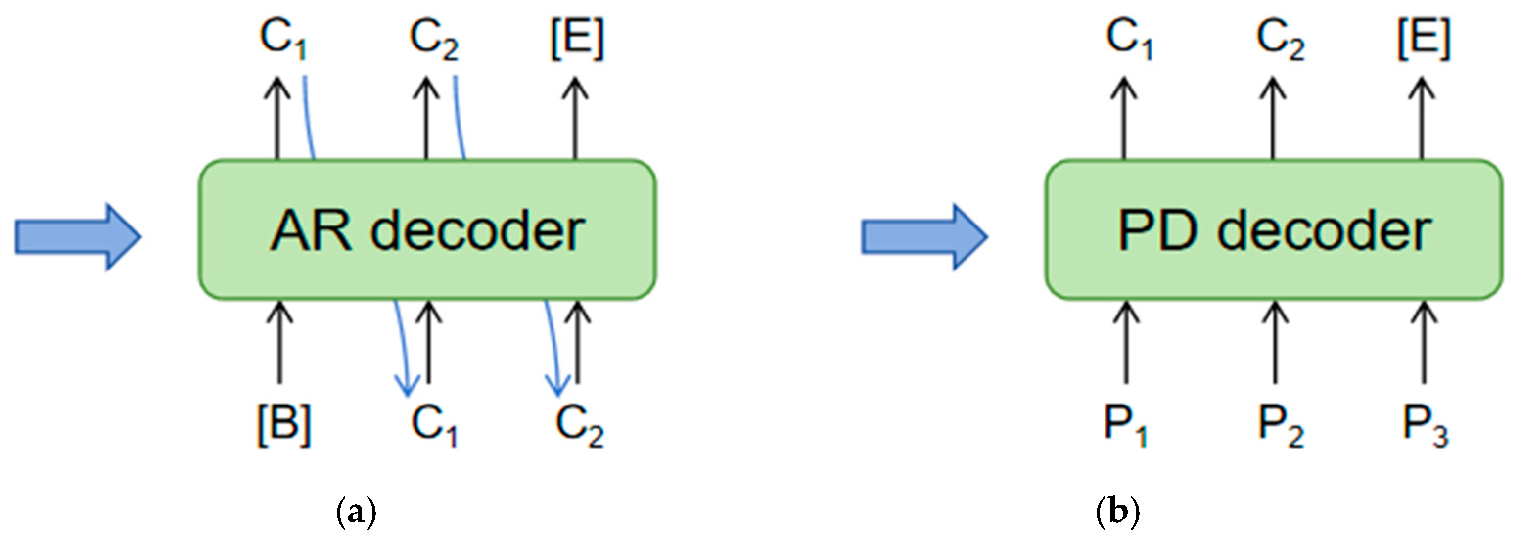
Figure 3.
Illustrates the AR and PD decoders: (a) represents the Auto-Regressive (AR) decoder, while (b) depicts the Parallel Decoding (PD) decoder. The blue arrows indicate visual features.
Figure 3.
Illustrates the AR and PD decoders: (a) represents the Auto-Regressive (AR) decoder, while (b) depicts the Parallel Decoding (PD) decoder. The blue arrows indicate visual features.
Figure 4.
Illustrates the overall architecture of our proposed text font correction and alignment method. F represents the original features extracted by the backbone, while Fc denotes the masked features obtained after processing through the DSTF. represents the features obtained from the fusion and alignment of F and Fc in the FACF. In the overall architecture, the English meaning of the Chinese image is the fire alarm device.
Figure 5.
Illustrates the structure of the Dual Attention Series Module (DASM) integrated between each residual block.
Figure 5.
Illustrates the structure of the Dual Attention Series Module (DASM) integrated between each residual block.
Figure 6.
Overall structure diagram after inserting DASM into FPN.
Figure 6.
Overall structure diagram after inserting DASM into FPN.
Figure 7.
Shows the structure of the Feature Alignment and Complementary Fusion (FACF). In this module, a set of reference points is uniformly placed across the feature map, and the offset is learned by concatenating the recognition features F and the features Fc obtained from the Discriminating Standard Text Font (DSTF) module. This offset guides the alignment of the two feature sets. The reference points (red, yellow, and green) are evenly distributed across the recognition feature map, and the offsets are learned from the concatenated features of the recognition and normalized maps.
Figure 8.
Highlights the differences between the custom VBC dataset and public datasets. In panels (
a–
c), the scenarios represent daytime, nighttime, and occlusion conditions, respectively, from top to bottom [
32,
35]. In panel (
b), from top to bottom, the Chinese translations are “Lis”, “Xiumei Cave”, and “Four Seasons Flowering Period”. In panel (
c), from top to bottom, the Chinese translations are “Teahouse Alley”, “Hairdressing”, and “Television”.
Figure 9.
Visualization of attention heatmaps. For each example, the heatmaps, from left to right, represent the baseline model, the attention heatmap using a ResNet-34 encoder, and the attention heatmap using a PlainMamba encoder. Here, “GT” represents the ground truth, “pred” represents the prediction from our model, and the top left corner shows the original image.
Figure 10.
Visualization of text recognition results in three challenging scenarios: arbitrary text arrangements, irregular text shapes, and unexpected font occlusions. Specifically, (1) illustrates arbitrary text arrangements in the ICDAR 2015 dataset, (2) depicts irregular text shapes in the SVT dataset, and (3) shows unexpected font occlusions in the custom VBC dataset. For each image, the text region displays the recognition results, with (
a,
b) showing the results compared to other models, and (
c) presenting the results of our proposed model. Red highlights indicate incorrectly recognized parts, while black highlights show correctly recognized parts [
4,
43]. The column in (3) is in Chinese, with the English translation as “storefront transfer”.
Figure 11.
Comparison of Average Accuracy (%), Parameter Count, and FPS of different models across datasets.
Figure 11.
Comparison of Average Accuracy (%), Parameter Count, and FPS of different models across datasets.
Figure 12.
Visualization of text regions after encoding. For each example, the original image is displayed on top, and the heatmap generated by the PlainMamba encoder is shown below it. The two images below are in Chinese, with the English translations, from left to right, as “Chaozhou Beef Hotpot” and “Haidao Forest Management Bureau”.
Figure 13.
Visualization of the results after ablating each module on the VBC dataset. For each example, the text instances obtained using the Text Font Correction and Alignment Method, along with their recognition results, are presented. From left to right, the three columns show the visualizations of the recognition features: using PlainMamba with DASM, using DSTF and FACF, and the final recognition features. Since VBC is a Chinese dataset, the attention heatmaps displayed are all in Chinese. In the first row, from left to right, the English translations are “Shanghai Research Institute” and “Yuanchang Xifuli”. In the second row, from left to right, the English translations are "Guangdong Regional General Agent, Guangzhou Dahe Machinery is recruiting agents in various cities and counties" and "Guangzhou Jiang Beer Co., Ltd”.
Figure 14.
Visualization of text recognition results, where (a–c) represent three different datasets, demonstrating the usefulness of each module in our method. The text areas next to each image, from top to bottom, represent the baseline model, the addition of DASM, the replacement of the encoder with PlainMamba, the combination of the DSTF and FACF modules, and the overall recognition performance of the model architecture. Red regions indicate recognition errors, while black regions represent correctly identified areas. The images in (a,c) contain Chinese text. In (a), the English meanings of the first row, from left to right, are “Serenity Leads to Greatness” and “Zhenmei Trading Hebei Co., Ltd”. The second row translates to “Hongli Bathhouse” and “Beauty Salon”. In (c), the English meanings of the first row, from left to right, are “Yadi” and “Experimental Base”. The second row translates to “Alliance Underfloor Heating Specialist” and “Air Conditioning Maintenance and Repair”.
Figure 15.
Shows the visualization of the text font masks generated by the model without refinement. The text region on the right side of the image displays the ground truth at the top and the predicted results at the bottom.
Figure 15.
Shows the visualization of the text font masks generated by the model without refinement. The text region on the right side of the image displays the ground truth at the top and the predicted results at the bottom.
Table 1.
Structure of the lightweight segmentation module with depth-wise convolution. The configuration outlines the components at the current stage: DepthConv represents depth-wise convolution, BN denotes batch normalization, and FC refers to the fully connected layer.
Table 1.
Structure of the lightweight segmentation module with depth-wise convolution. The configuration outlines the components at the current stage: DepthConv represents depth-wise convolution, BN denotes batch normalization, and FC refers to the fully connected layer.
| Layer | Configuration |
|---|
| Stage 1 | DepthConv |
| BN |
| Stage 2, Stage 3 and Stage 4 | Upsample |
| DepthConv |
| BN |
| ReLU |
| DepthConv |
| BN |
| FC | - |
Table 2.
This section presents experiments using different datasets to validate the feasibility of both the theoretical and practical approaches for the recognizer and binarization decoder. The bolded numbers indicate better performance on these datasets.
Table 2.
This section presents experiments using different datasets to validate the feasibility of both the theoretical and practical approaches for the recognizer and binarization decoder. The bolded numbers indicate better performance on these datasets.
| CTC Recognizer | Binarization Decoder | VBC | ICDAR2013 | SVT | ICDAR2015 | SVTP | Average Accuracy (%) |
|---|
| ✔ | | 89.9 | 97.5 | 95.8 | 88.2 | 92.8 | 92.8 |
| ✔ | ✔ | 90.8 | 98.3 | 97.1 | 89.5 | 93.4 | 93.8 |
Table 3.
Comparison of dataset differences in scene text recognition.
Table 3.
Comparison of dataset differences in scene text recognition.
| Benchmarks | Test Images | Description | Language | Light Condition |
|---|
| ICDAR2013 [33] | 1015 | Regular Scene Text | English | Daytime and standard lighting conditions |
| SVT [34] | 647 | Regular Scene Text | English | Daytime and standard lighting conditions |
| ICDAR2015 [35] | 1811 | Irregular scene text | English | Daytime and standard lighting conditions |
| SVTP [36] | 645 | Irregular scene text | English | Variations in lighting, including sunlight and shadows |
| CTR [32] Scene | 63,645 | Irregular scene text | Chinese | Natural sunlight, indoor lighting, and some uneven lighting |
| CTR [32] Web | 14,589 | Regular Scene Text | Chinese | Natural sunlight |
| CTR [32] Document | 50,000 | Regular Scene Text | Chinese | Natural sunlight, indoor lighting |
| CTR [32] Handwriting | 23,389 | Irregular scene text | Chinese | Natural sunlight, indoor lighting |
| IC2017-MLT [38] | 1200 | Irregular scene text | Multilingualism | Variations in lighting, including sunlight, indoor lighting, and shadows |
| IC2019-ArT [39] | 4573 | Irregular scene text | Chinese + English | Natural and artificial light sources |
| COCO-TEXT [37] | 7026 | Irregular scene text | English | Various lighting conditions, including daytime, dusk, and nighttime |
| CTW1500 [40] | 2000 | Irregular scene text | Chinese + English | Strong light, reflections, shadows, and nighttime scenes |
| MSRA-TD500 [41] | 1500 | Regular Scene Text | Chinese + English | Daytime and nighttime |
| VBC | 2613 | Irregular scene text | Chinese | Scenes captured under different natural lighting conditions |
Table 4.
Comparison of our method with other advanced models on the VBC and English datasets. The evaluation metrics are accuracy and average accuracy. Bold fonts indicate the best performance, while “_” denotes the second-best performance.
Table 4.
Comparison of our method with other advanced models on the VBC and English datasets. The evaluation metrics are accuracy and average accuracy. Bold fonts indicate the best performance, while “_” denotes the second-best performance.
| Method | Encoder | Input Size | VBC | ICDAR2013 | SVT | ICDAR2015 | SVTP | Average Accuracy (%) |
|---|
| RobustScanner [42] | ResNet | 48 × 160 | 85.1 | 94.8 | 88.1 | 77.1 | 79.5 | 84.9 |
| CRNN [10] | ResNet+BiLSTM | 32 × 100 | 83.3 | 91.1 | 81.6 | 69.4 | 70.0 | 79.1 |
| SVTR-T [43] | SVTR-Tiny | 32 × 100 | 87.0 | 96.3 | 91.6 | 84.1 | 85.4 | 88.9 |
| CPPD [1] | SVTR-Base | 32 × 100 | 88.4 | 96.8 | 95.2 | 87.2 | 90.2 | 91.6 |
| PPOCR [44] | ResNet | 32 × 100 | 87.1 | 95.5 | 91.5 | 84.4 | 89.5 | 89.6 |
| PARSeq [2] | ViT | 32 × 128 | 88.0 | 97.0 | 93.6 | 86.5 | 88.9 | 90.8 |
| SRN [23] | ResNet+FPN | 64 × 256 | 86.8 | 95.5 | 91.5 | 82.7 | 85.1 | 88.3 |
| CDistNet [22] | ResNet+En | 32 × 128 | 88.1 | 97.4 | 93.5 | 86.0 | 88.7 | 90.7 |
| I2C2W [3] | ResNet+En | 64 × 600 | 86.7 | 95.0 | 91.7 | 82.8 | 83.1 | 87.9 |
| LPV-B [4] | SVTR-Base | 48 × 160 | 88.6 | 97.6 | 94.6 | 87.5 | 90.9 | 91.8 |
| Ours1 | ResNet | 32 × 128 | 89.8 | 97.4 | 96.0 | 87.1 | 92.1 | 92.5 |
| Ours2 | PlainMamba | 32 × 128 | 90.8 | 98.3 | 97.1 | 89.5 | 93.4 | 93.8 |
Table 5.
Efficiency comparison across different models. Bold fonts indicate the best performance, while “_” denotes the second-best performance.
Table 5.
Efficiency comparison across different models. Bold fonts indicate the best performance, while “_” denotes the second-best performance.
| Method | Encoder | Average Accuracy (%) | Parameters (×106) | FPS |
|---|
| RobustScanner [42] | ResNet | 84.9 | 48.0 | 16.4 |
| CRNN [10] | ResNet+BiLSTM | 79.1 | 8.30 | 159 |
| SVTR-T [43] | SVTR-Tiny | 88.9 | 6.03 | 408 |
| CPPD [1] | SVTR-Base | 91.6 | 24.6 | 212 |
| PPOCR [44] | ResNet | 89.6 | 8.6 | - |
| PARSeq [2] | ViT | 90.8 | 23.8 | 84.7 |
| SRN [23] | ResNet+FPN | 88.3 | 54.7 | 39.4 |
| CDistNet [22] | ResNet+En | 90.7 | 65.5 | 14.5 |
| I2C2W [3] | ResNet+En | 87.9 | - | - |
| LPV-B [4] | SVTR-Base | 91.8 | 35.1 | 103 |
| Ours1 | ResNet | 92.5 | 13.2 | 154 |
| Ours2 | PlainMamba | 93.8 | 17.6 | 136 |
Table 6.
Comparison of our model with others on the VBC and public datasets with metrics from [
45]. The evaluation metrics are CER and WER, where smaller values indicate better performance. Bold fonts indicate the best performance, while “_” denotes the second-best performance.
Table 6.
Comparison of our model with others on the VBC and public datasets with metrics from [
45]. The evaluation metrics are CER and WER, where smaller values indicate better performance. Bold fonts indicate the best performance, while “_” denotes the second-best performance.
| Methods | IC2017-MLT | IC2019-ArT | COCO-TEXT | CTW1500 | MSRA-TD500 |
|---|
| CER | WER | CER | WER | CER | WER | CER | WER | CER | WER |
|---|
| Wang [46] | 0.11 | 0.14 | 0.09 | 0.18 | 0.18 | 0.13 | 0.11 | 0.14 | 0.05 | 0.18 |
| Qiao [47] | 0.18 | 0.12 | 0.17 | 0.18 | 0.12 | 0.11 | 0.18 | 0.12 | 0.17 | 0.18 |
| ABCNet [48] | 0.17 | 0.12 | 0.17 | 0.13 | 0.12 | 0.11 | 0.17 | 0.12 | 0.17 | 0.13 |
| PAN++ [49] | 0.14 | 0.06 | 0.17 | 0.09 | 0.14 | 0.08 | 0.14 | 0.16 | 0.17 | 0.17 |
| Ours | 0.03 | 0.06 | 0.07 | 0.05 | 0.09 | 0.07 | 0.03 | 0.05 | 0.04 | 0.06 |
Table 7.
Compares our method with SOTA methods with the results of the comparison methods obtained from [
32]. Bold fonts indicate the best performance, while “_” denotes the second-best performance.
Table 7.
Compares our method with SOTA methods with the results of the comparison methods obtained from [
32]. Bold fonts indicate the best performance, while “_” denotes the second-best performance.
| Method | Venue | Scene | Web | Document | Handwriting | Average Accuracy (%) |
|---|
| CRNN [10] | TPAMI2017 | 54.9 | 56.2 | 97.4 | 48.0 | 64.1 |
| ASTER [17] | TPAMI2019 | 59.4 | 57.8 | 91.6 | 45.9 | 63.7 |
| MORAN [50] | PR2019 | 54.7 | 49.6 | 91.7 | 30.2 | 56.6 |
| SAR [16] | AAAI2019 | 53.8 | 50.5 | 96.2 | 31.0 | 57.9 |
| SEED [51] | CVPR2020 | 45.4 | 31.4 | 96.1 | 21.1 | 48.5 |
| MASTER [52] | PR2021 | 62.1 | 53.4 | 82.7 | 18.5 | 54.2 |
| ABINet [24] | CVPR2021 | 60.9 | 51.1 | 91.7 | 13.8 | 54.4 |
| TransOCR [53] | CVPR2021 | 67.8 | 62.7 | 97.9 | 51.7 | 70.0 |
| CCR-CLIP [54] | ICCV2023 | 71.3 | 69.2 | 98.3 | 60.3 | 74.8 |
| CPPD [1] | CVPR2023 | 78.4 | 79.3 | 98.9 | 57.6 | 78.6 |
| CAM-Base [55] | CVPR2024 | 78.0 | 69.8 | 98.3 | 61.1 | 76.8 |
| Ours1 | - | 79.2 | 78.5 | 99.1 | 60.7 | 79.4 |
| Ours2 | - | 80.7 | 80.3 | 99.5 | 61.4 | 80.5 |
Table 8.
Comparison of results using three different encoders on the VBC dataset. In all cases, DASM is used in the feature extraction stage, although its position may vary. Bold fonts indicate the best performance.
Table 8.
Comparison of results using three different encoders on the VBC dataset. In all cases, DASM is used in the feature extraction stage, although its position may vary. Bold fonts indicate the best performance.
| Encoder | Accuracy (%) | Parameters (×106) | FPS |
|---|
| Ours-ResNet | 88.6 | 11.8 | 163 |
| Ours-ResNet-DASM | 89.8 | 13.2 | 154 |
| Ours-SVTR-Base | 89.1 | 21.4 | 132 |
| Ours-SVTR-Base-DASM | 90.0 | 23.0 | 128 |
| Ours-PlainMamba | 90.3 | 16.8 | 152 |
| Ours-PlainMamba-DASM | 90.8 | 17.6 | 136 |
Table 9.
Recognition accuracy under different lighting conditions. Bold fonts indicate the best performance.
Table 9.
Recognition accuracy under different lighting conditions. Bold fonts indicate the best performance.
| Different Light Conditions | VBC |
|---|
| Strong light | 84.4 |
| Weak light | 82.7 |
| Lamplight | 89.5 |
| Darkness | 73.2 |
Table 10.
Comparison of our model with other models on Chinese–English mixed datasets. The performance metrics of other models are from [
45] and the evaluation metric used is accuracy. Bold fonts indicate the best performance, while “_” denotes the second-best performance.
Table 10.
Comparison of our model with other models on Chinese–English mixed datasets. The performance metrics of other models are from [
45] and the evaluation metric used is accuracy. Bold fonts indicate the best performance, while “_” denotes the second-best performance.
| Methods | IC2019-ArT | CTW1500 | MSRA-TD500 | Average Accuracy (%) |
|---|
| Wang [46] | 87.5 | 86.2 | 86.5 | 86.7 |
| Qiao [47] | 83.3 | 84.0 | 82.3 | 83.2 |
| ABCNet [48] | 81.4 | 81.2 | 80.4 | 81.0 |
| PAN++ [49] | 89.6 | 89.4 | 89.6 | 89.5 |
| Ours | 92.4 | 92.7 | 93.2 | 92.8 |
Table 11.
Presents the ablation study of the individual units of the model. Bold fonts indicate the best performance.
Table 11.
Presents the ablation study of the individual units of the model. Bold fonts indicate the best performance.
| Dual Attention Serial Module (DASM) | Discriminative Standard Text Font (DSTF) Module | Feature Alignment and Complementary Fusion (FACF) Module | PlainMamba | VBC | ICDAR2015 | SVTP |
|---|
| | | | | 87.1 | 84.4 | 89.5 |
| | | | ✔ | 88.4 | 86.5 | 91.1 |
| ✔ | | | | 88.0 | 84.8 | 90.2 |
| ✔ | | | ✔ | 88.9 | 86.7 | 91.8 |
| | ✔ | ✔ | | 88.6 | 85.3 | 90.9 |
| ✔ | ✔ | ✔ | | 89.5 | 86.9 | 92.1 |
| | ✔ | ✔ | ✔ | 90.2 | 88.1 | 92.9 |
| ✔ | ✔ | ✔ | ✔ | 90.8 | 89.5 | 93.4 |


