
In-Motion Forward–Forward Backtracking Fine Alignment Based on Displacement Observation for SINS/GNSS


Abstract
1. Introduction
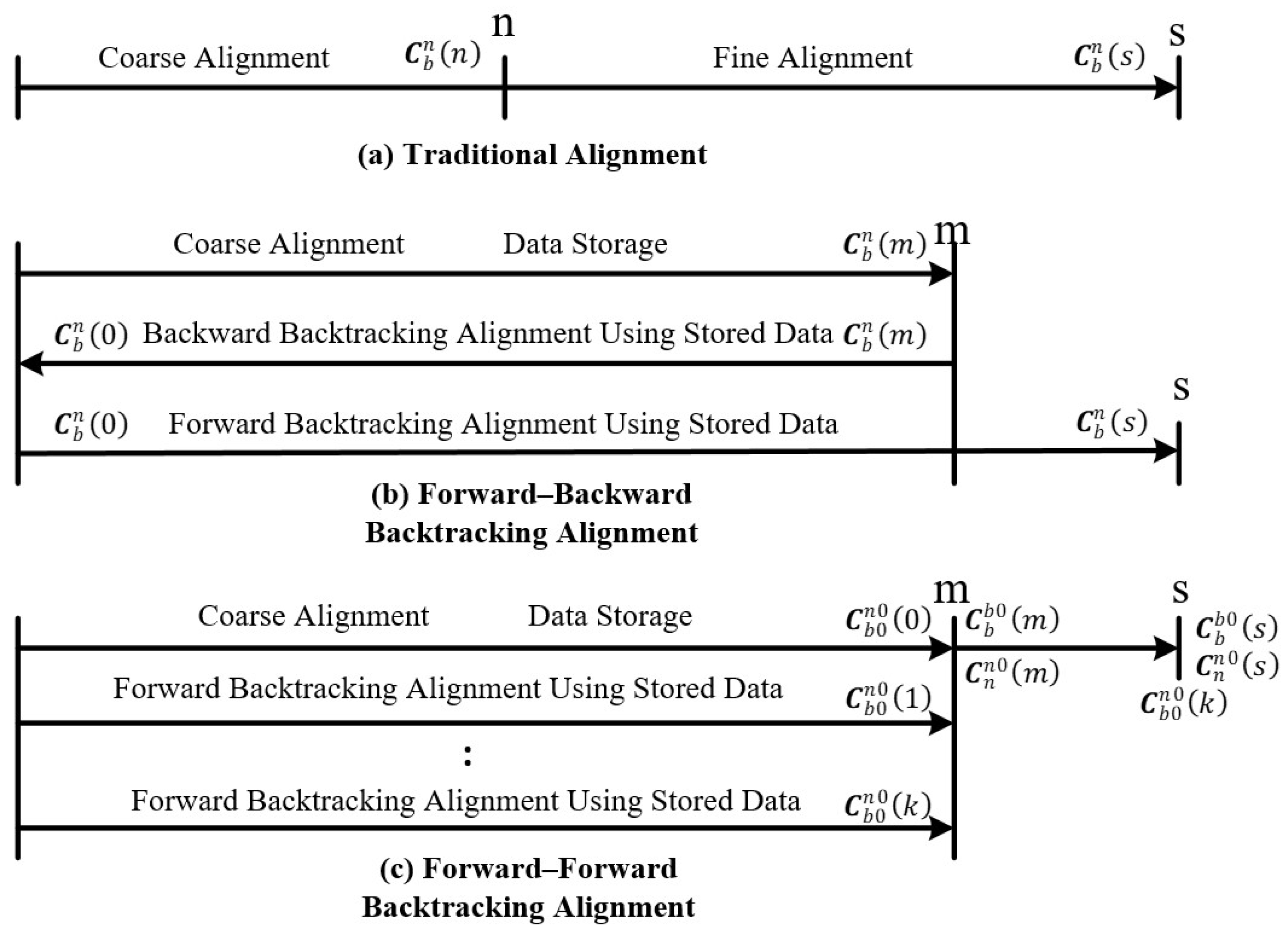
2. The Error Model of Backtracking Fine Alignment Based on an Inertial Frame
2.1. State Equation of Backtracking Alignment
2.2. Measurement Equation of Backtracking Alignment
3. Simulation Test
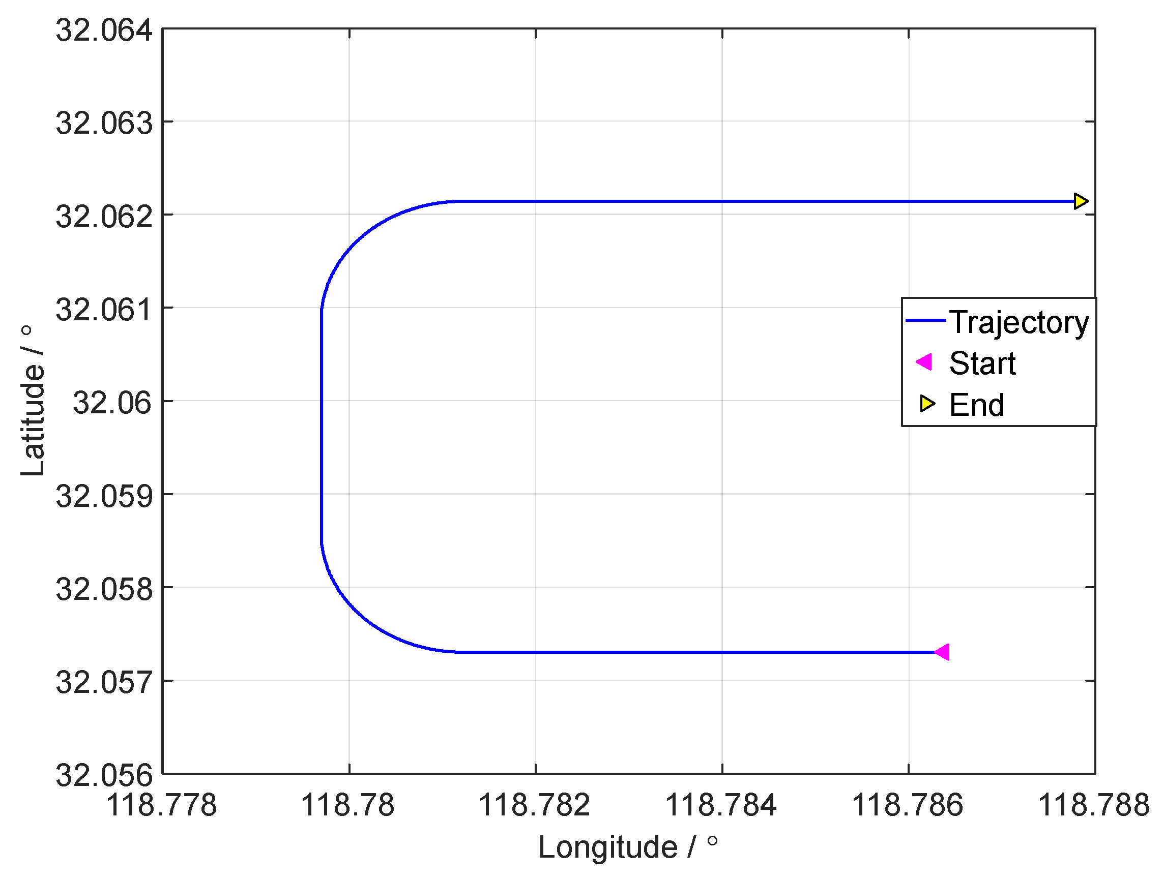
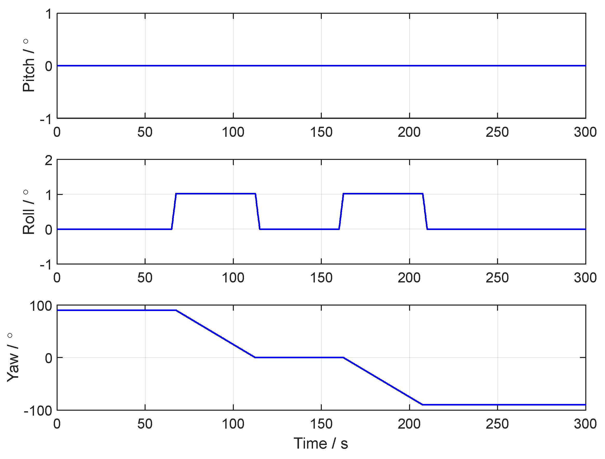
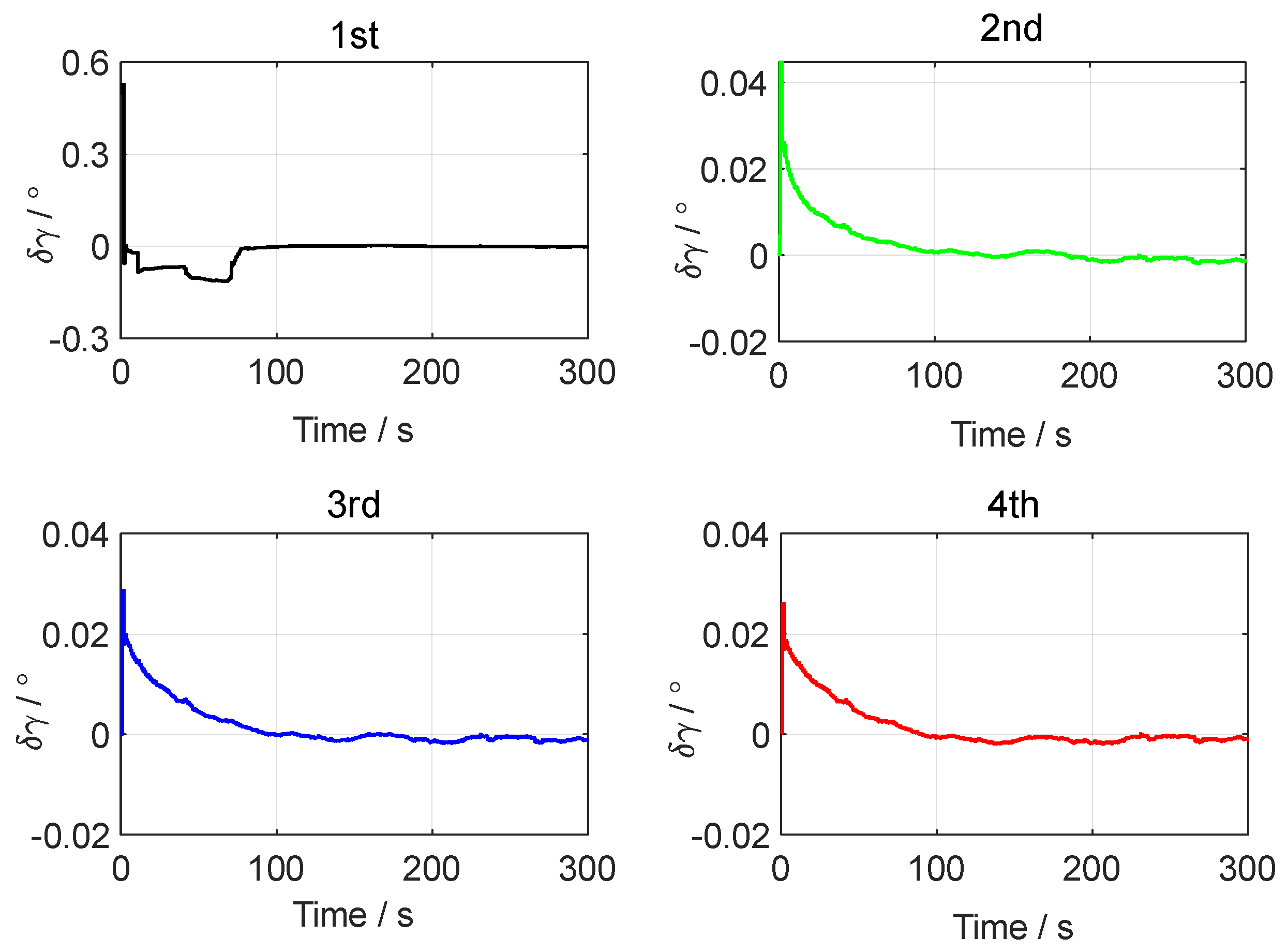
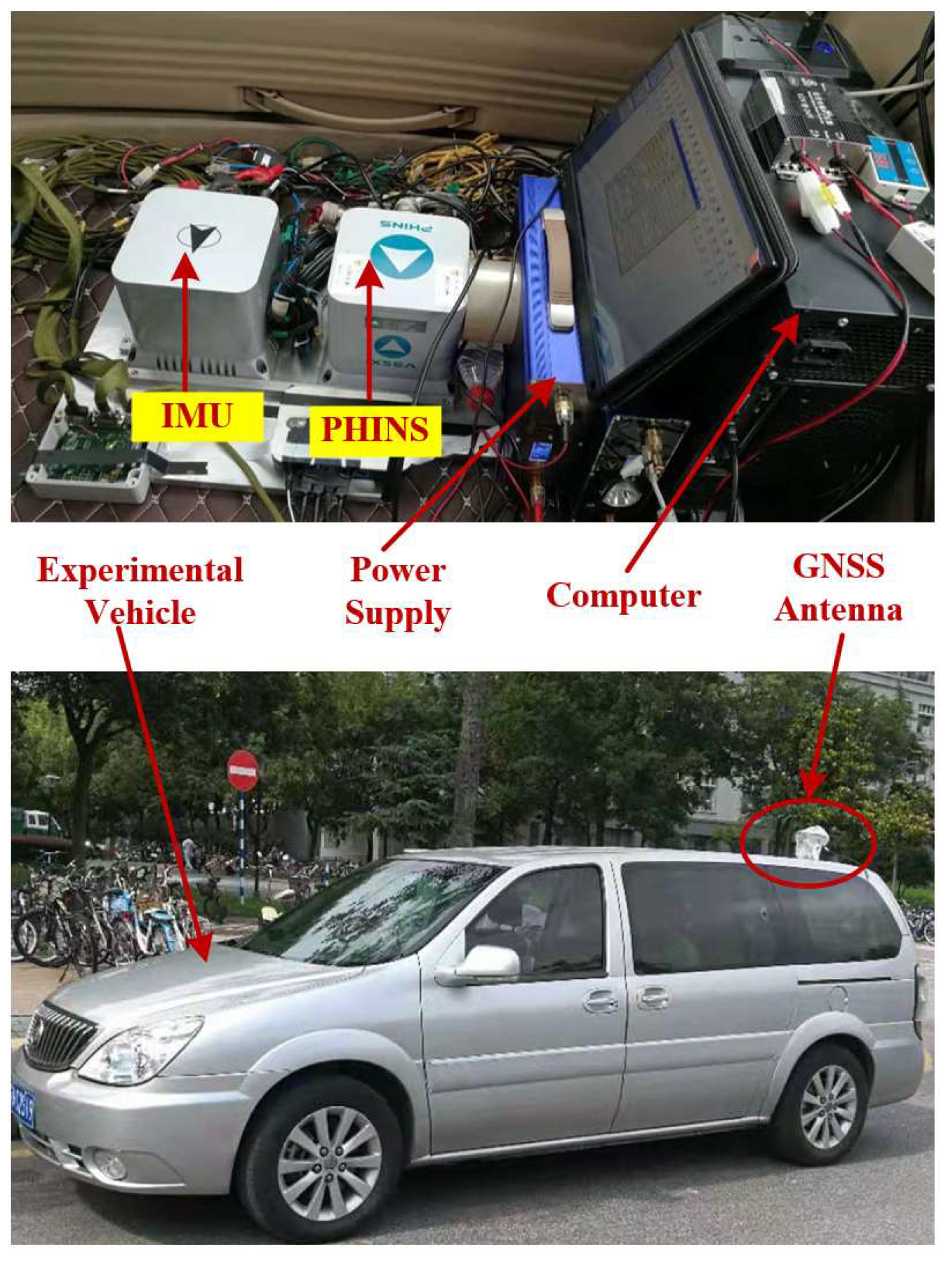
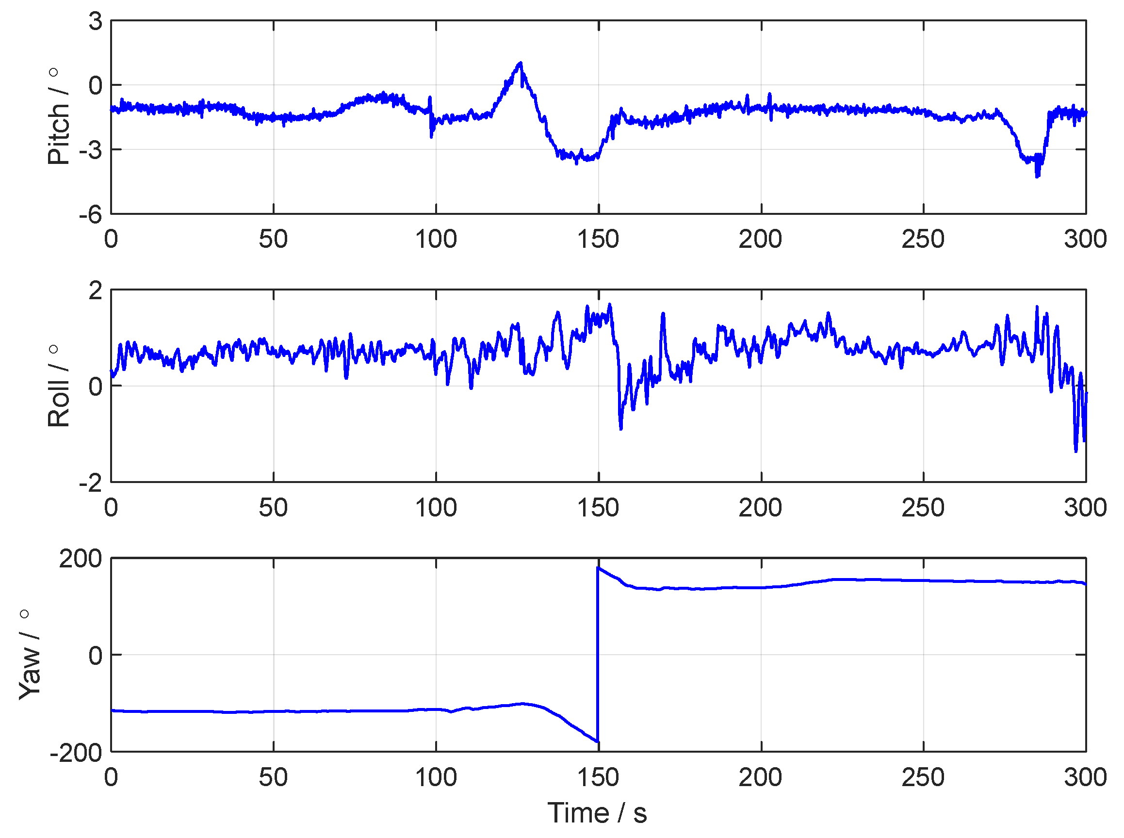
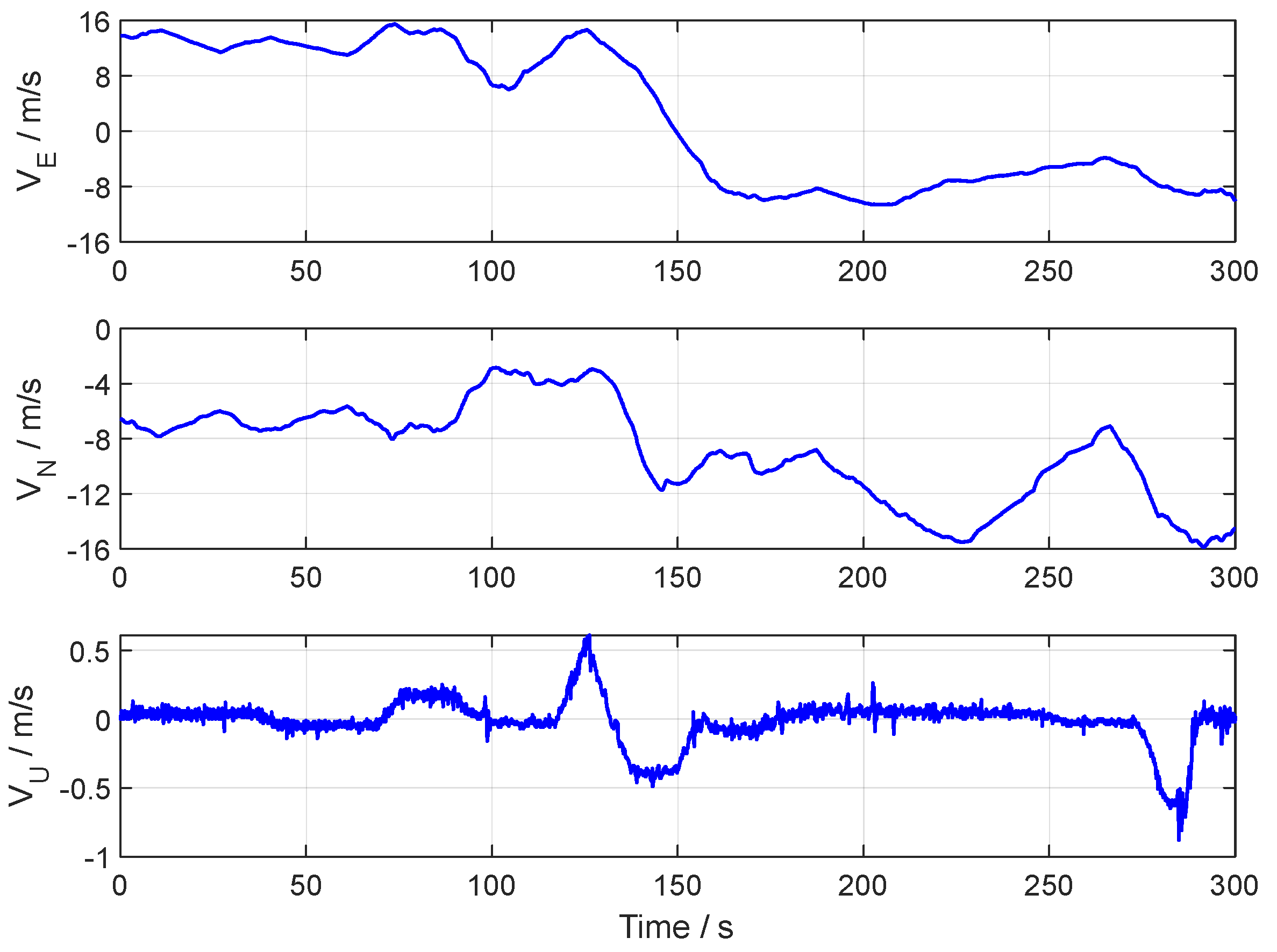
4. Vehicle Test
5. Conclusions
Author Contributions
Funding
Data Availability Statement
Conflicts of Interest
References
- Sánchez, M.; Morales, J.; Martínez, J.L. Reinforcement and curriculum learning for off-road navigation of an UGV with a 3D LiDAR. Sensors 2023, 23, 3239. [Google Scholar] [CrossRef] [PubMed]
- Baras, N.; Dasygenis, M. UGV Coverage Path Planning: An Energy-Efficient Approach through Turn Reduction. Electronics 2023, 12, 2959. [Google Scholar] [CrossRef]
- Ma, C.; Pan, S.G.; Gao, W.; Ye, F.; Liu, L.W.; Wang, H. Improving GNSS/INS tightly coupled positioning by using BDS-3 four-frequency observations in urban environments. Remote Sens. 2022, 14, 615. [Google Scholar] [CrossRef]
- Li, X.; Liang, J.W.; Huang, G.W.; Ma, S.H.; Li, H. Adaptive Invariant Extended Kalman Filter-Based Tightly-Coupled SINS/RTK Integrated Positioning for Rotor Unmanned Aerial Vehicle. IEEE Trans. Instrum. Meas. 2024, 73, 1–17. [Google Scholar] [CrossRef]
- Zhang, H.Z.; Yang, X.T.; Liang, J.S.; Xu, X.; Sun, X.Q. GPS path tracking control of military unmanned vehicle based on preview variable universe fuzzy sliding mode control. Machines 2021, 9, 304. [Google Scholar] [CrossRef]
- Cui, B.B.; Chen, W.; Weng, D.J.; Wei, X.H.; Sun, Z.Y.; Zhao, Y.; Liu, Y.F. Observability-constrained resampling-free cubature Kalman filter for GNSS/INS with measurement outliers. Remote Sens. 2023, 15, 4591. [Google Scholar] [CrossRef]
- Geng, X.S.; Guo, Y.; Tang, K.H.; Wu, W.Q.; Ren, Y.C.; Duan, G.D. A Covert Spoofing Algorithm for SINS/GNSS Tightly Integrated Navigation System. IEEE Trans. Autom. Sci. Eng. 2024, 73, 1–9. [Google Scholar] [CrossRef]
- Li, Y.C.; Feng, F.; Cai, Y.F.; Li, Z.X.; Sotelo, M.A. Localization for intelligent vehicles in underground car parks based on semantic information. IEEE trans. Intell. Transp. Syst. 2023, 25, 1317–1332. [Google Scholar] [CrossRef]
- Arafat, M.Y.; Alam, M.M.; Moh, S. Vision-based navigation techniques for unmanned aerial vehicles: Review and challenges. Drones 2023, 7, 89. [Google Scholar] [CrossRef]
- Tang, C.Y. Non-initial attitude error analysis of SINS by error closed-loop and energy-level constructing. Aerosp. Sci. Technol. 2020, 106, 106149. [Google Scholar] [CrossRef]
- Wang, D.; Wang, B.; Huang, H.Q.; Yao, Y.Q. An Improved Robust Filter Method for SINS/DVL System with Earth Frame Error Model. IEEE Trans. Veh. Technol. 2024, 73, 12760–12772. [Google Scholar] [CrossRef]
- Jing, H.; Gao, Y.; Shahbeigi, S.; Dianati, M. Integrity monitoring of GNSS/INS based positioning systems for autonomous vehicles: State-of-the-art and open challenges. IEEE Trans. Intell. Transp. Syst. 2022, 23, 14166–14187. [Google Scholar] [CrossRef]
- Luo, Q.; Cao, Y.R.; Liu, J.J.; Benslimane, A. Localization and navigation in autonomous driving: Threats and countermeasures. IEEE Wirel. Commun. 2019, 26, 38–45. [Google Scholar] [CrossRef]
- Lyu, X.; Hu, B.Q.; Wang, Z.; Gao, D.Y.; Li, K.L.; Chang, L.B. A SINS/GNSS/VDM integrated navigation fault-tolerant mechanism based on adaptive information sharing factor. IEEE Trans. Instrum. Meas. 2022, 71, 1–13. [Google Scholar] [CrossRef]
- Xiang, Z.Y.; Zhang, T.; Wang, Q.; Jin, S.L.; Nie, X.M.; Duan, C.F.; Zhou, J. A SINS/GNSS/2D-LDV integrated navigation scheme for unmanned ground vehicles. Meas. Sci. Technol. 2023, 34, 125116. [Google Scholar] [CrossRef]
- Xu, X.; Li, Y.; Zhu, L.H.; Yao, Y.Q. Robust attitude and positioning alignment methods for SINS/DVL integration based on sliding window improvements. IEEE Trans. Ind. Electron. 2023, 71, 8038–8046. [Google Scholar] [CrossRef]
- Cui, B.B.; Wei, X.H.; Chen, X.Y.; Li, J.Y.; Li, L. On sigma-point update of cubature Kalman filter for GNSS/INS under GNSS-challenged environment. IEEE Trans. Veh. Technol. 2019, 68, 8671–8682. [Google Scholar] [CrossRef]
- Yao, Y.Q.; Xu, X.; Zhang, T.; Hu, G.G. An improved initial alignment method for SINS/GPS integration with vectors subtraction. IEEE Sens. J. 2021, 21, 18256–18262. [Google Scholar] [CrossRef]
- Luo, L.; Huang, Y.L.; Zhang, Z.; Zhang, Y.G. A new Kalman filter-based in-motion initial alignment method for DVL-aided low-cost SINS. IEEE Trans. Veh. Technol. 2021, 70, 331–343. [Google Scholar] [CrossRef]
- Chang, L.B.; Qin, F.J.; Xu, J.N. Strapdown inertial navigation system initial alignment based on group of double direct spatial isometries. IEEE Sens. J. 2021, 22, 803–818. [Google Scholar] [CrossRef]
- Xu, X.; Sun, Y.F.; Gui, J.; Yao, Y.Q.; Zhang, T. A fast robust in-motion alignment method for SINS with DVL aided. IEEE Trans. Veh. Technol. 2020, 69, 3816–3827. [Google Scholar] [CrossRef]
- Xu, B.; Ding, W.J.; Wang, L.Z. A Robust FOAM Initial Alignment Method for SINS Assisted by DVL. IEEE Trans. Instrum. Meas. 2024, 73, 8504610. [Google Scholar] [CrossRef]
- Xu, X.; Ning, X.L.; Yao, Y.Q.; Li, K. In-motion coarse alignment method for SINS/GPS integration in polar region. IEEE Trans. Veh. Technol. 2022, 71, 6110–6118. [Google Scholar] [CrossRef]
- Liu, W.Q.; Cheng, X.H.; Ding, P.; Cao, P. An optimal indirect in-motion coarse alignment method for GNSS-aided SINS. IEEE Sens. J. 2022, 22, 7608–7618. [Google Scholar] [CrossRef]
- Chen, Y.M.; Li, W.; Wang, Y.Q. A robust adaptive indirect in-motion coarse alignment method for GPS/SINS integrated navigation system. Measurement 2021, 172, 108834. [Google Scholar] [CrossRef]
- Xu, X.; Zheng, X.H.; Li, Y.; Yao, Y.Q.; Zhou, H.; Zhu, L.H. An improved in-motion alignment method for SINS/GPS with the sliding windows integration. IEEE Trans. Veh. Technol. 2023, 72, 12491–12499. [Google Scholar] [CrossRef]
- Cao, S.Y.; Gao, H.L.; Yi, Y. Adaptive in-flight alignment method for SINS/GPS/polarization integrated navigation system based on the degree of observability analysis. IEEE Sens. J. 2023, 23, 16699–16709. [Google Scholar] [CrossRef]
- Zhou, X.R.; Zhang, M.; Hu, J.C.; Li, L.; Guan, X.H. A Robust In-Motion Coarse Alignment Method for Low-Accuracy SINS and GPS Integrated System. IEEE ASME Trans. Mechatron. 2024; early access. [Google Scholar] [CrossRef]
- Zhu, Y.Y.; Zhang, T.; Cui, B.B.; Wei, X.H.; Jin, B.N. In-Motion Coarse Alignment for SINS/USBL Based on USBL Relative Position. IEEE Trans. Autom. Sci. Eng. 2024. early access. [Google Scholar] [CrossRef]
- Chang, L.B.; Qin, F.J.; Li, A. A novel backtracking scheme for attitude determination-based initial alignment. IEEE Trans. Autom. Sci. Eng. 2014, 12, 384–390. [Google Scholar] [CrossRef]
- Lin, Y.S.; Miao, L.J.; Zhou, Z.Q. A high-accuracy initial alignment method based on backtracking process for strapdown inertial navigation system. Measurement 2022, 201, 111712. [Google Scholar] [CrossRef]
- Wang, J.W.; Chen, X.Y.; Liu, J.G.; Zhu, X.F.; Zhong, Y.L. A robust backtracking CKF based on Krein space theory for in-motion alignment process. IEEE trans. Intell. Transp. Syst. 2022, 24, 1909–1925. [Google Scholar] [CrossRef]
- Xu, X.; Xu, D.C. A Forward Forward Backtracking Alignment Method for SINS on Swaying Base. J. Astronaut. 2019, 40, 965. [Google Scholar]
- Wei, X.K.; Li, J.; Feng, K.Q.; Zhang, D.B. An Improved In-flight Alignment Method Based on Backtracking Navigation for GPS-aided Low Cost SINS With Short Endurance. IEEE Robot. Autom. Lett. 2021, 7, 634–641. [Google Scholar] [CrossRef]
- Sun, Y.D.; Wang, L.F.; Cai, Q.Z.; Yang, G.L.; Wen, Z.Y. In-motion attitude and position alignment for odometer-aided SINS based on backtracking scheme. IEEE Access 2019, 7, 20211–20224. [Google Scholar] [CrossRef]


| Sensor | Parameters | Value |
|---|---|---|
| IMU | Gyroscope biases | 0.02 °/h |
| Gyroscope random noise | 0.005 °/√h | |
| Accelerometer biases | 500 μg | |
| Accelerometer random noise | 50 μg/√Hz | |
| Output frequency | 200 Hz | |
| GPS | Positioning error | 10 m |
| Speed error | 0.5 m/s | |
| Output frequency | 1 Hz |
| Order | Time (s) | Motion State | Order | Time (s) | Motion State |
|---|---|---|---|---|---|
| 1 | 0–10 | 7 | 160–205 | Turning right, w = 2 °/s | |
| 2 | 10–40 | Uniform motion | 8 | 205–225 | Uniform motion |
| 3 | 40–45 | 9 | 225–230 | ||
| 4 | 45–65 | Uniform motion | 10 | 230–255 | Uniform motion |
| 5 | 65–110 | Turning right, w = 2 °/s | 11 | 255–260 | |
| 6 | 110–160 | Uniform motion | 12 | 260–300 | Uniform motion |
| Sensor | Parameters | Value |
|---|---|---|
| Gyroscope | Constant biases | <0.02 ) |
| Random noise | <0.005 °/√h | |
| Measurement range | ±300 °/s | |
| Output frequency | 200 Hz | |
| Accelerometer | Constant biases | <5 × |
| Random noise | <5 × | |
| Measurement range | ±20 g | |
| Output frequency | 200 Hz |
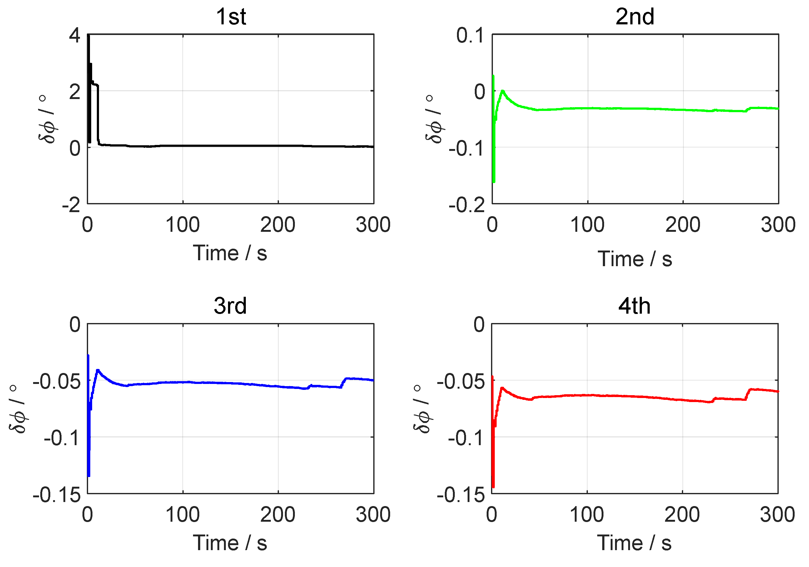
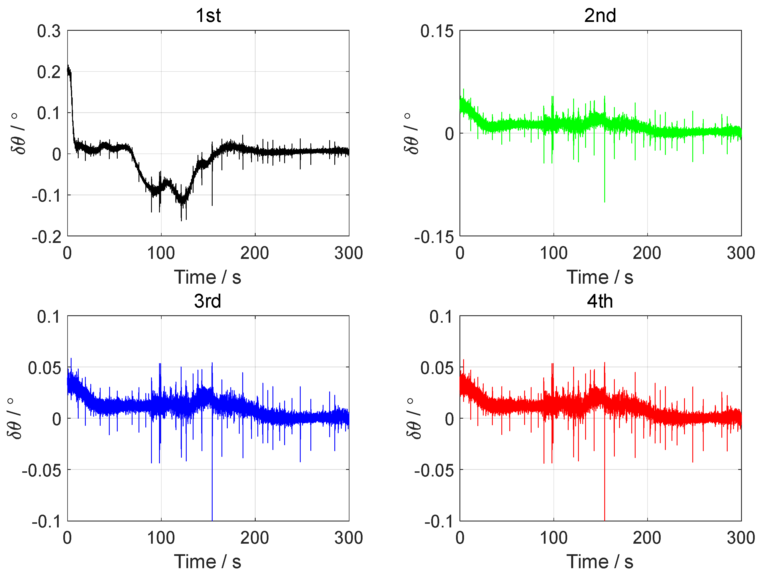
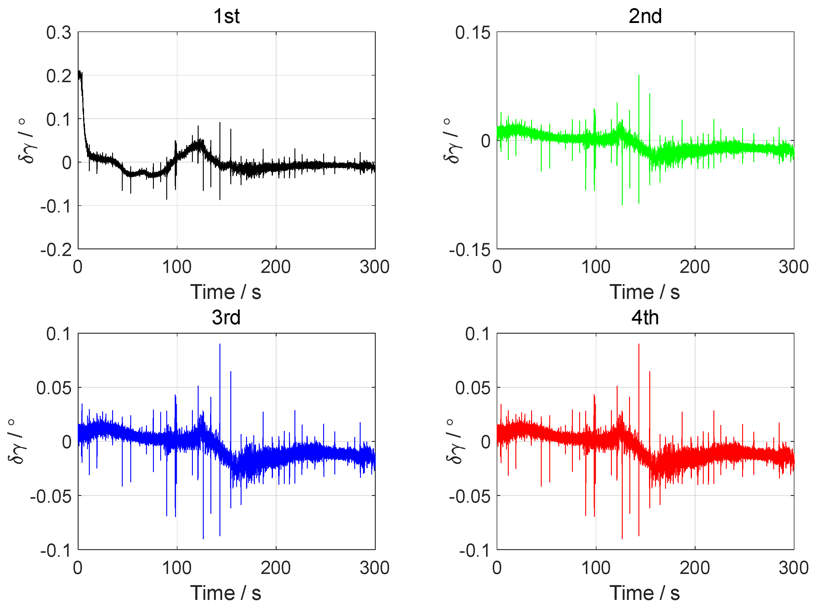
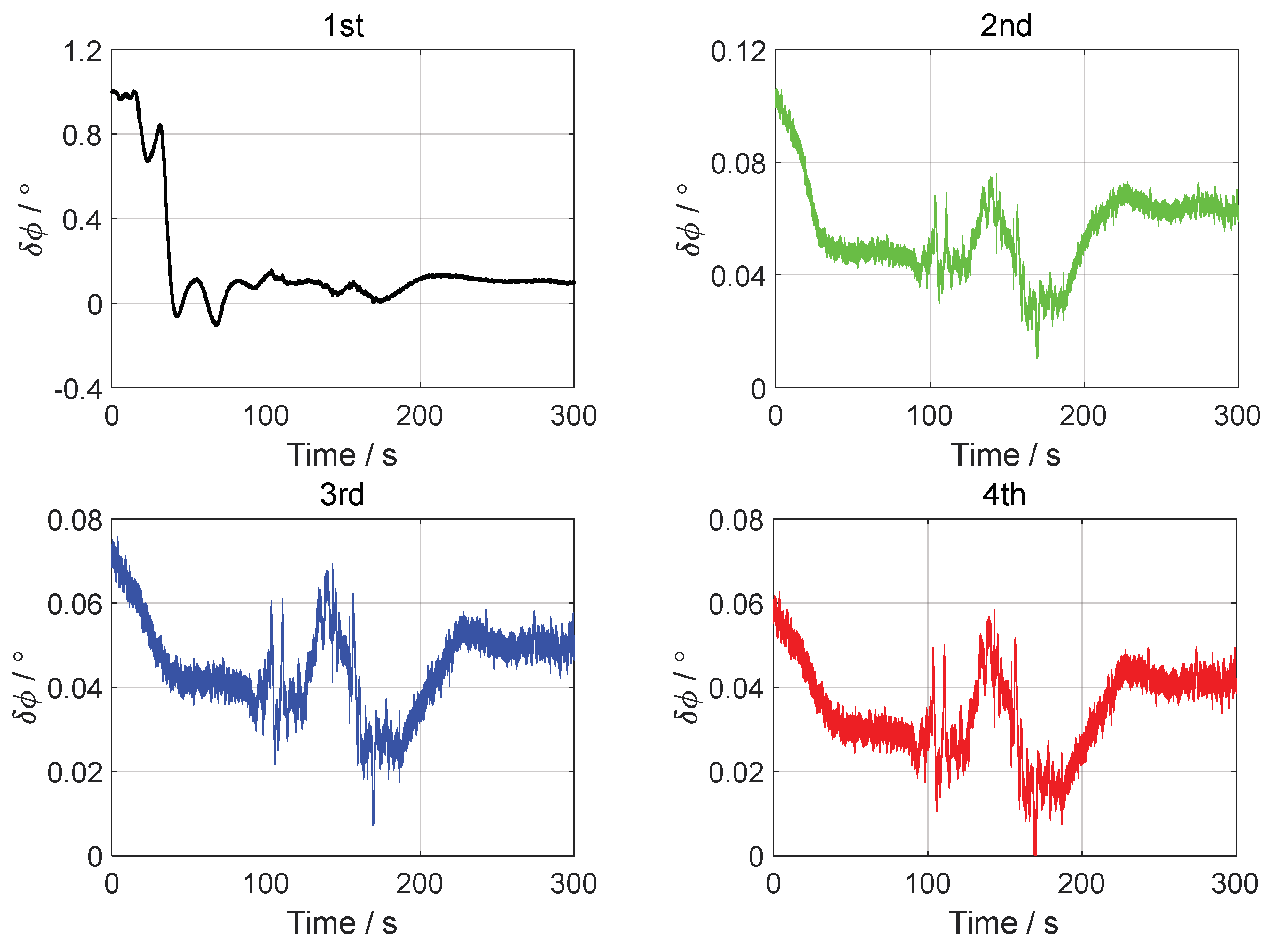
| Order | Error | Pitch | Roll | Yaw |
|---|---|---|---|---|
| 1st | MN (°) | 0.0055 | −0.0087 | 0.1114 |
| STD (°) | 0.0035 | 0.0038 | 0.0112 | |
| RMS (°) | 0.0065 | 0.0095 | 0.1120 | |
| 2nd | MN (°) | 0.0019 | −0.0116 | 0.0636 |
| STD (°) | 0.0034 | 0.0039 | 0.0036 | |
| RMS (°) | 0.0039 | 0.0123 | 0.0637 | |
| 3rd | MN (°) | 0.0012 | −0.0120 | 0.0489 |
| STD (°) | 0.0035 | 0.0039 | 0.0045 | |
| RMS (°) | 0.0037 | 0.0127 | 0.0491 | |
| 4th | MN (°) | 0.0010 | −0.0123 | 0.0400 |
| STD (°) | 0.0035 | 0.0040 | 0.0048 | |
| RMS (°) | 0.0037 | 0.0129 | 0.0403 |
Disclaimer/Publisher’s Note: The statements, opinions and data contained in all publications are solely those of the individual author(s) and contributor(s) and not of MDPI and/or the editor(s). MDPI and/or the editor(s) disclaim responsibility for any injury to people or property resulting from any ideas, methods, instructions or products referred to in the content. |
© 2024 by the authors. Licensee MDPI, Basel, Switzerland. This article is an open access article distributed under the terms and conditions of the Creative Commons Attribution (CC BY) license (https://creativecommons.org/licenses/by/4.0/).
Share and Cite
Zhu, Y.; Zhu, Y.; Wei, X.; Cui, B.; Liu, S. In-Motion Forward–Forward Backtracking Fine Alignment Based on Displacement Observation for SINS/GNSS. Sensors 2024, 24, 7916. https://doi.org/10.3390/s24247916
Zhu Y, Zhu Y, Wei X, Cui B, Liu S. In-Motion Forward–Forward Backtracking Fine Alignment Based on Displacement Observation for SINS/GNSS. Sensors. 2024; 24(24):7916. https://doi.org/10.3390/s24247916
Chicago/Turabian StyleZhu, Yongyun, Yaohui Zhu, Xinhua Wei, Bingbo Cui, and Shede Liu. 2024. "In-Motion Forward–Forward Backtracking Fine Alignment Based on Displacement Observation for SINS/GNSS" Sensors 24, no. 24: 7916. https://doi.org/10.3390/s24247916
APA StyleZhu, Y., Zhu, Y., Wei, X., Cui, B., & Liu, S. (2024). In-Motion Forward–Forward Backtracking Fine Alignment Based on Displacement Observation for SINS/GNSS. Sensors, 24(24), 7916. https://doi.org/10.3390/s24247916