
Pressure Sensors: Working Principles of Static and Dynamic Calibration


Abstract
1. Introduction
2. Pressure Measuring Principles
2.1. Bourdon Tube, Bellow, Diaphragm and Capsule
2.2. Piezoresistance and Strain Gauge
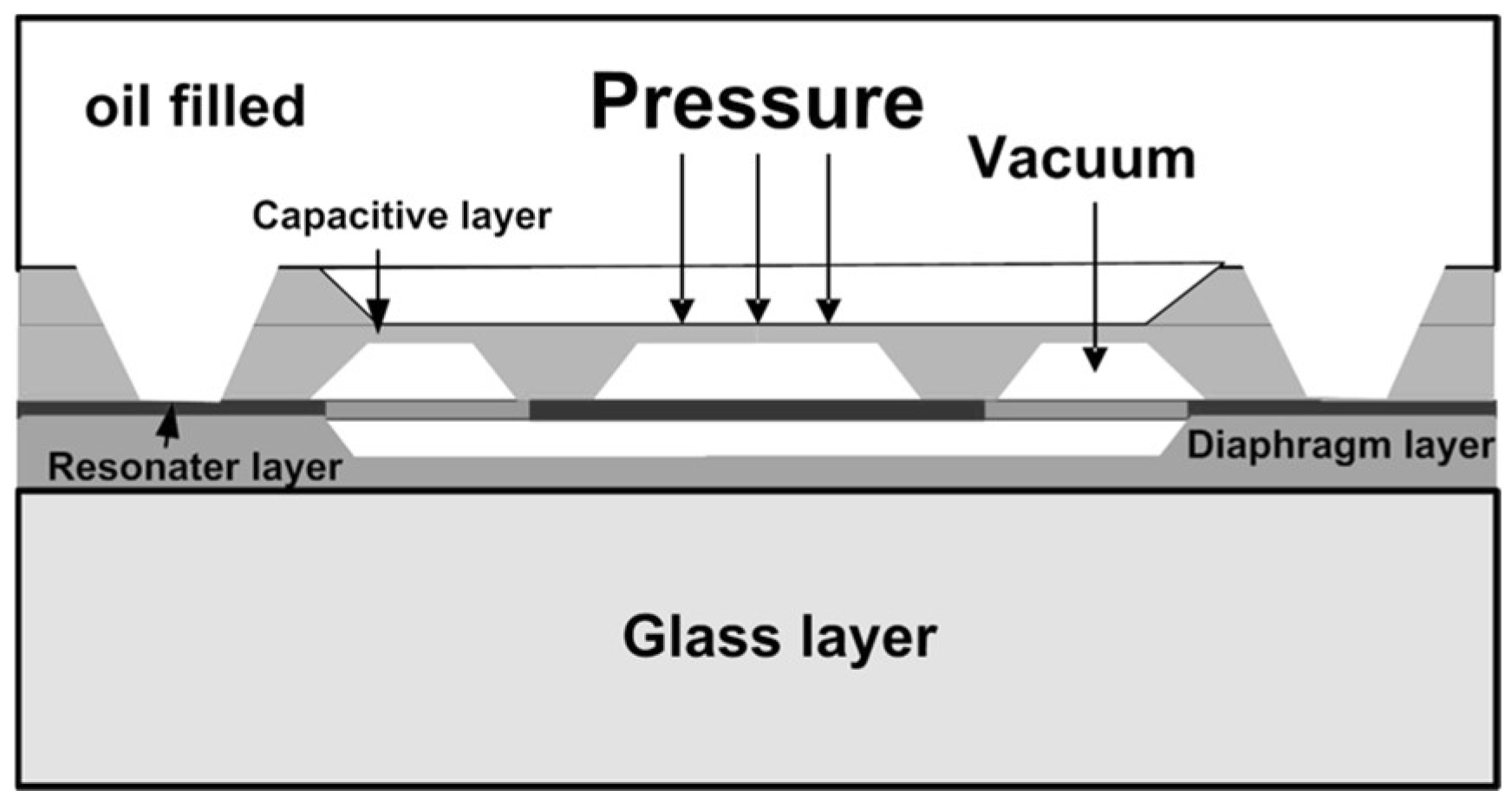
2.3. Capacitor
2.4. Reluctance
2.5. Piezoelectrics
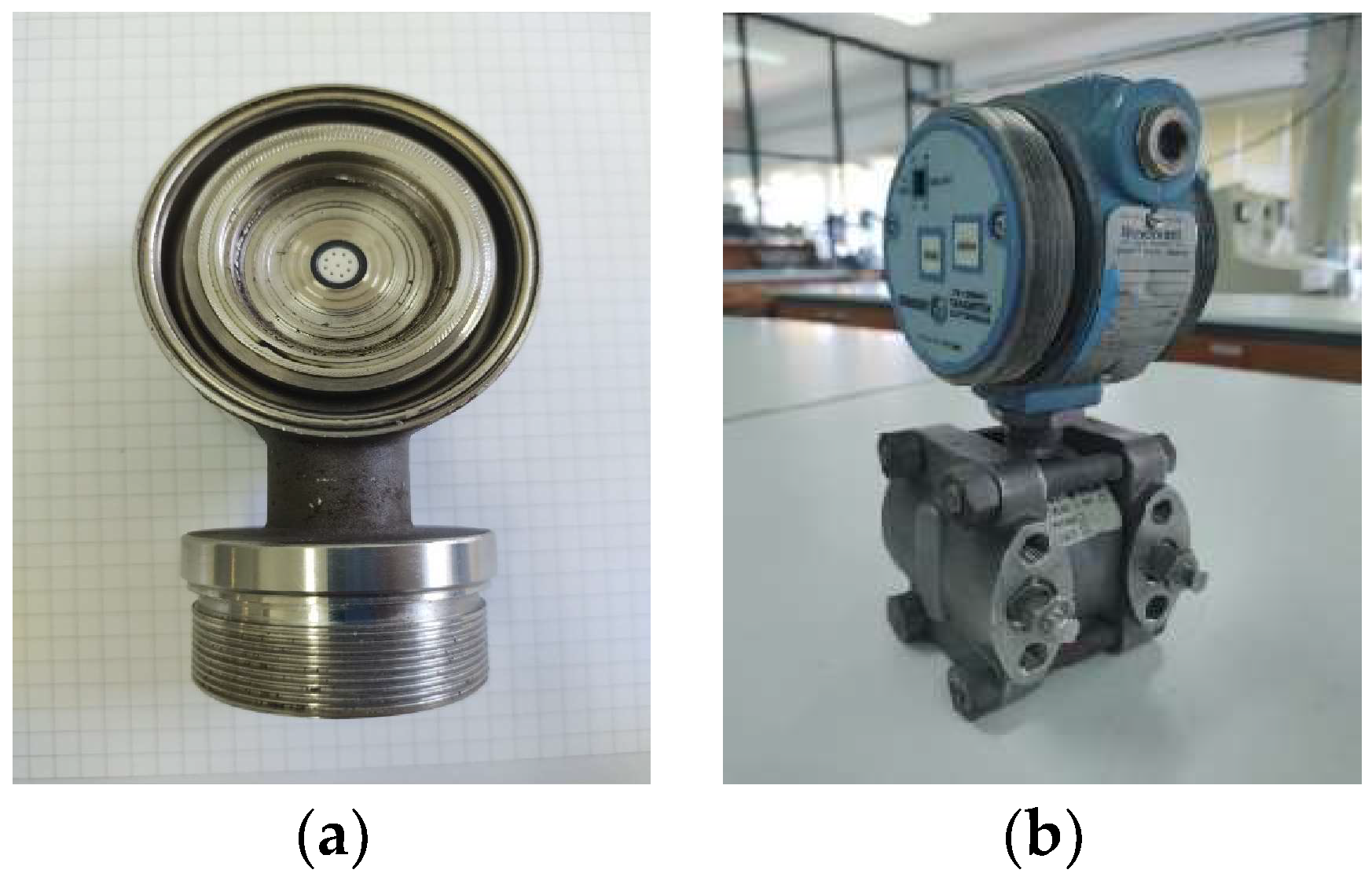
2.6. Resonance
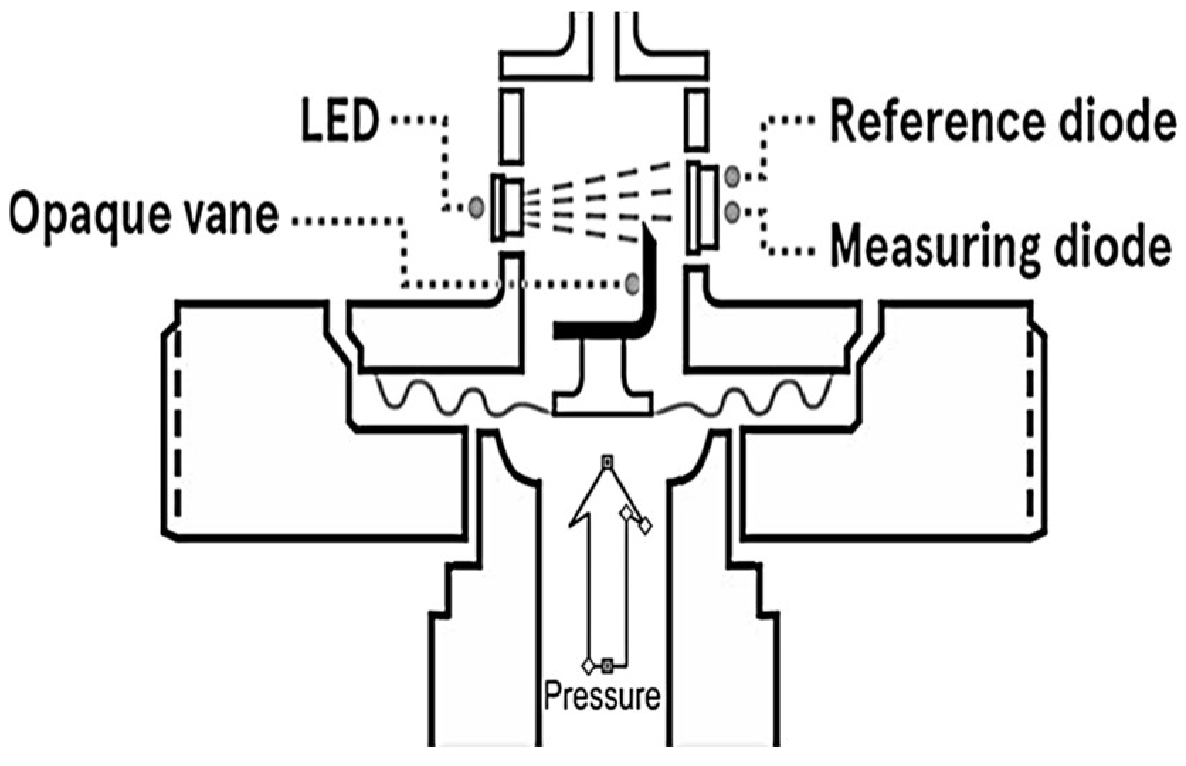
2.7. Optics
3. Calibration and Pressure Generators
3.1. Static Calibration
3.2. Dynamic Calibration
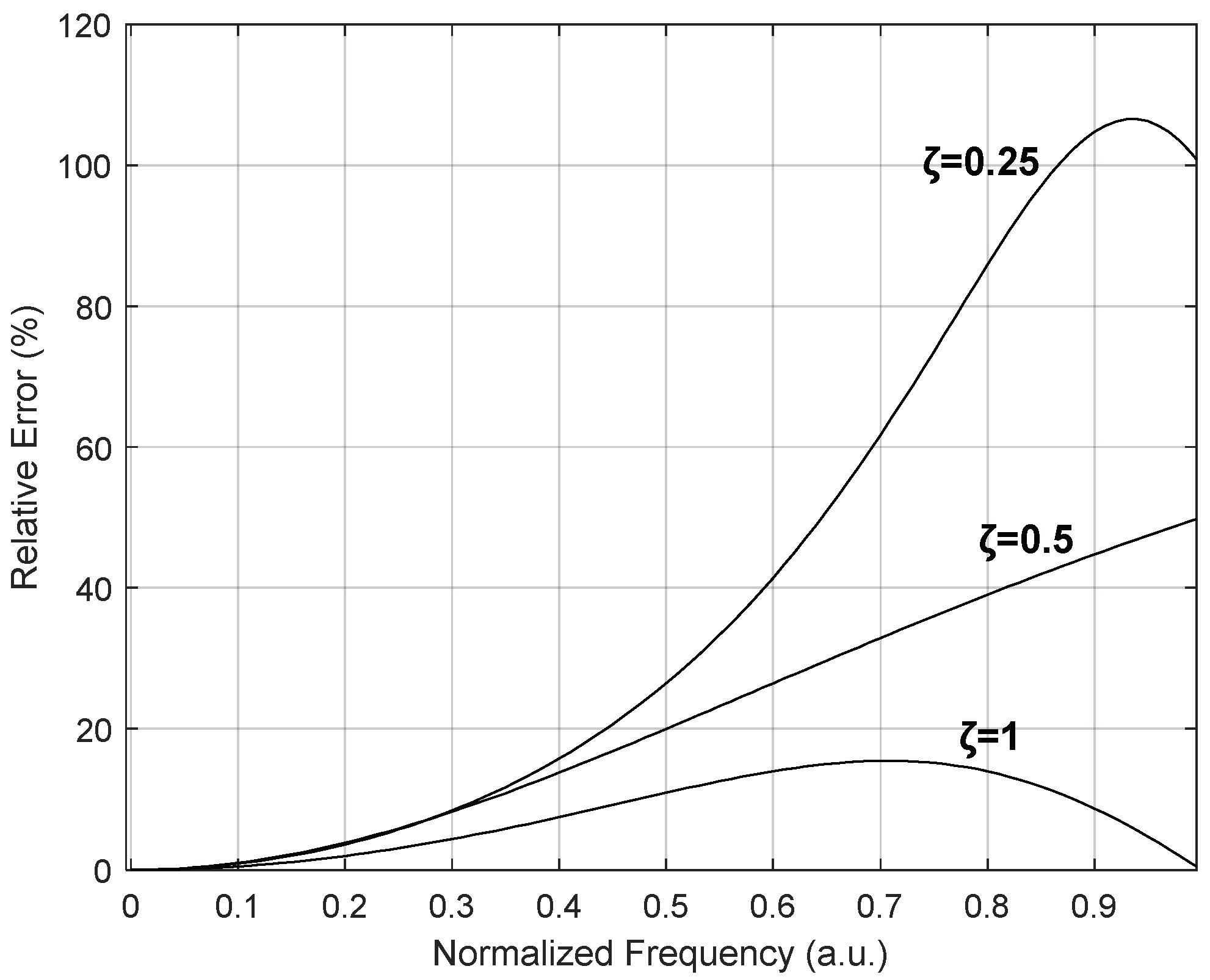
3.3. Pressure Measurement Channel and Transmitter Damping
3.4. Periodic Pressure Generators
3.5. Aperiodic Pressure Generators
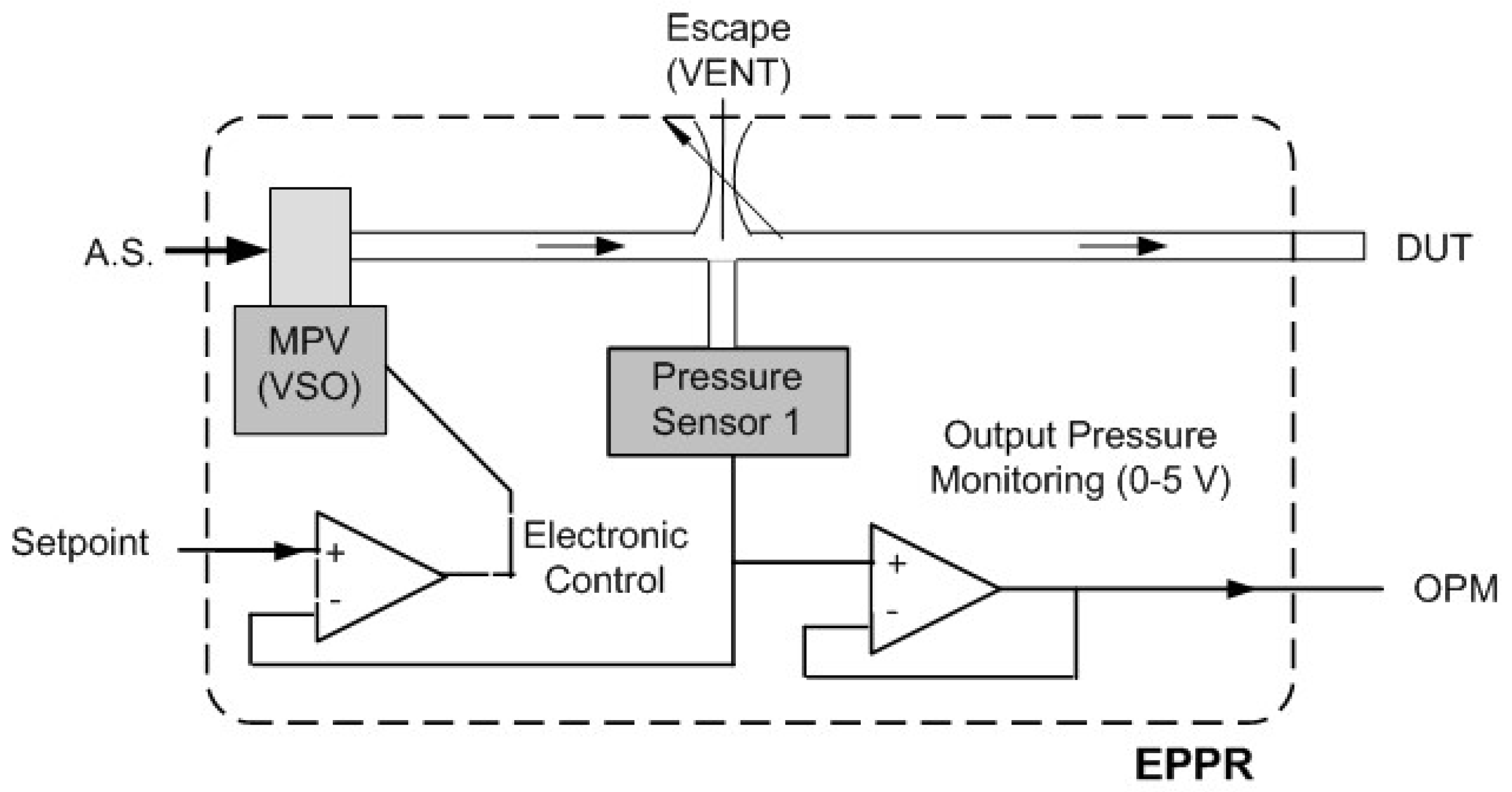
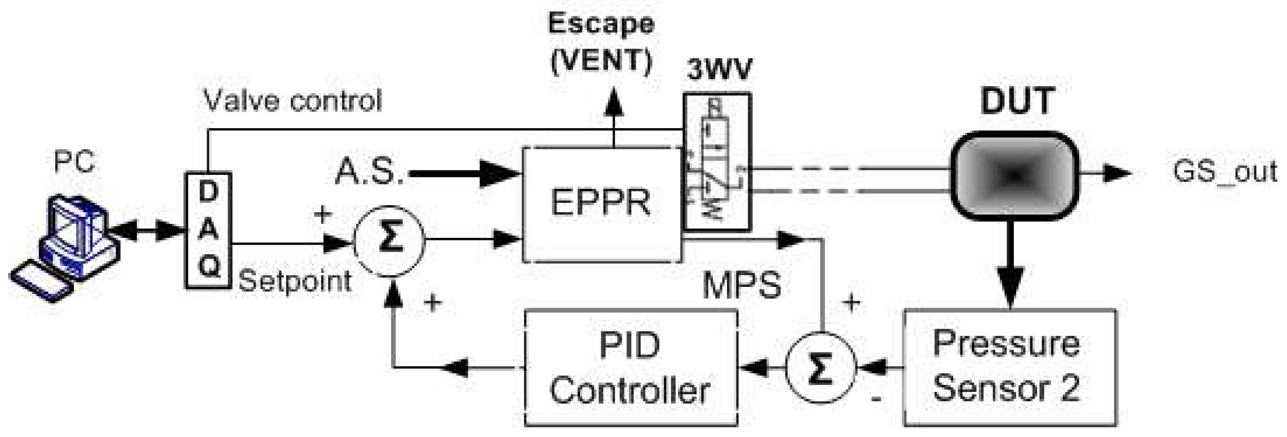
4. Proposed Calibration Prototype
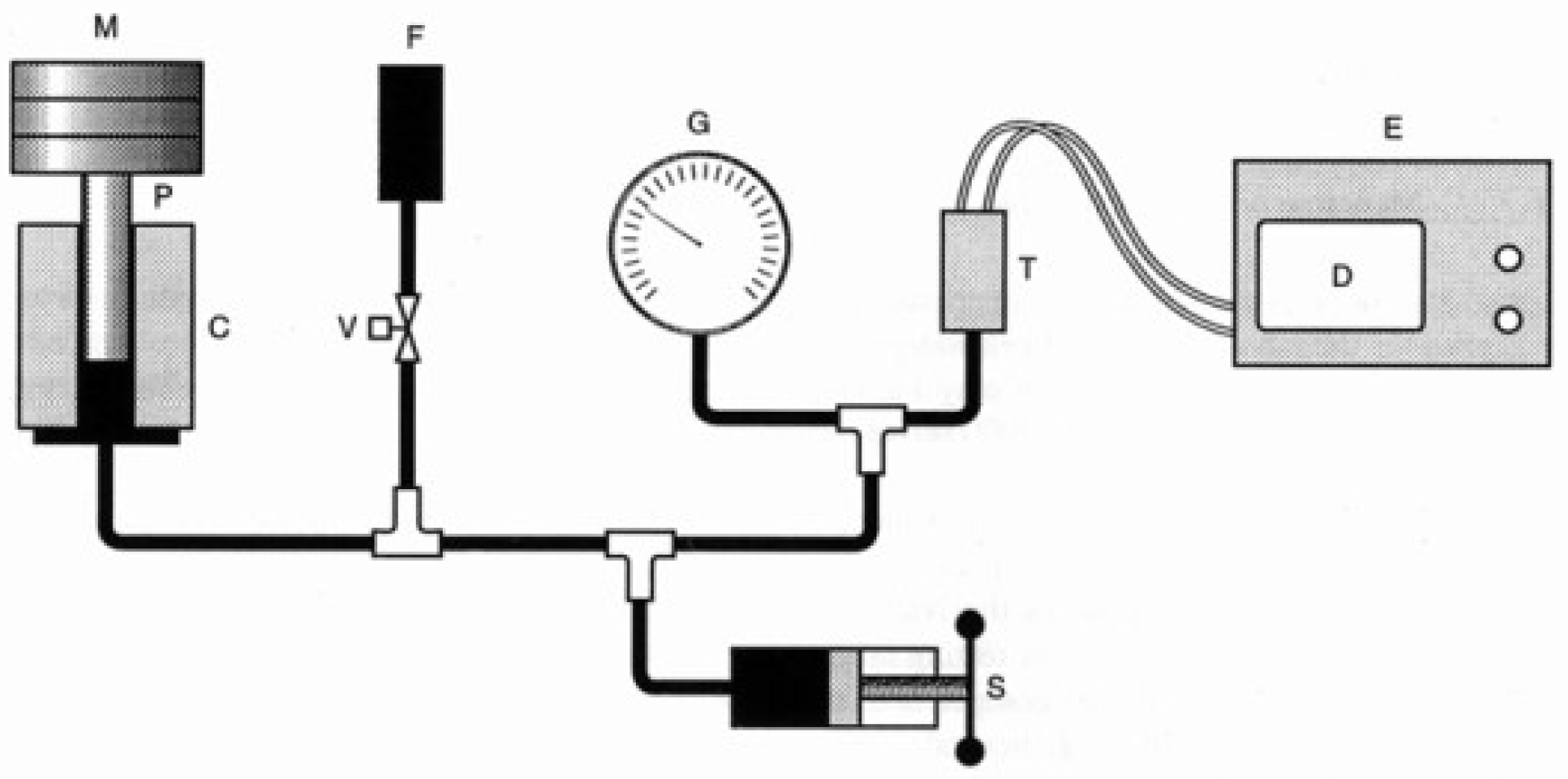
4.1. Hardware
4.2. Software
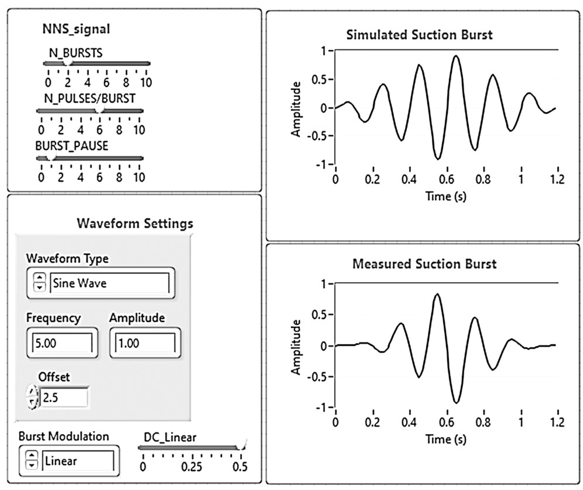
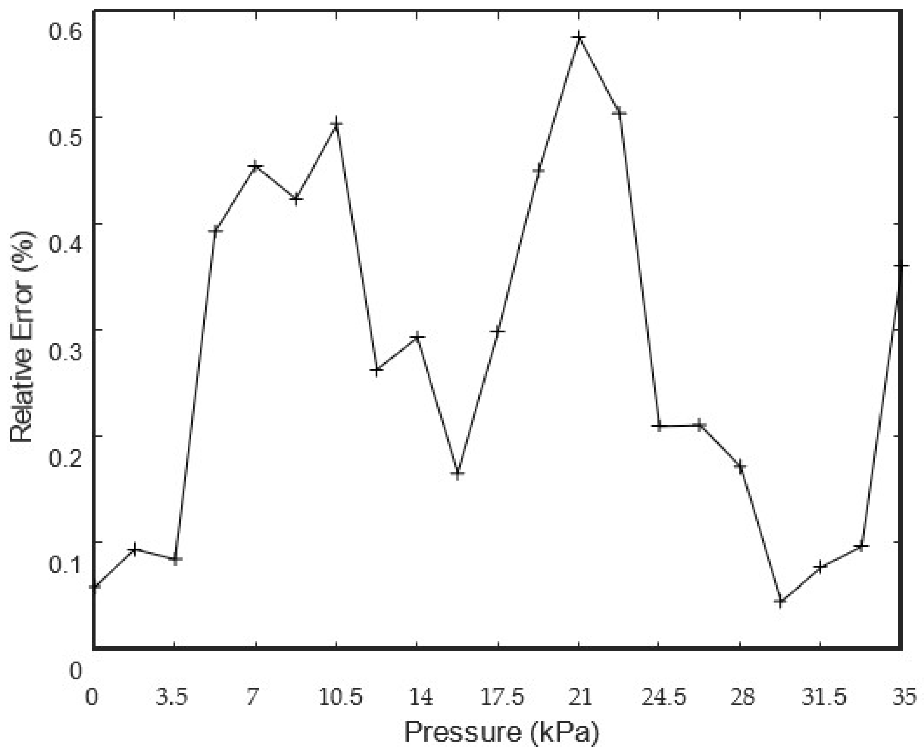
5. Experimental Results
5.1. Static and Dynamic Calibration of an Industrial Transmitter
5.2. Capillary Effects
6. Conclusions
Funding
Data Availability Statement
Conflicts of Interest
References
- TTan, M.; Lu, Y.; Wu, X.; Liu, H.; Tian, X. Investigation on performance of a centrifugal pump with multi-malfunction. J. Low Freq. Noise Vib. Act. Control. 2018, 40, 740–752. [Google Scholar] [CrossRef]
- Karvinen, T. Pulsation Analysis of Paper Making Process. Ph.D. Thesis, Tampere University of Technology, Tampere, Finland, 2007. Publication 657. [Google Scholar]
- Delgadillo, V.M.A.; Ramírez, P. Simultaneous pressure and level control of a combined cycle power plant deaerator. In Proceedings of the 54th ISA POWID Symposium, Charlotte, NC, USA, 5–10 June 2011; Volume 487, pp. 1–12. [Google Scholar]
- Shi, Y.; Kong, D.; Zhang, C. Research of a Sensor Used to Calculate the Dynamic Pressure of Chemical Explosions. IEEE Sens. J. 2021, 21, 27325–27334. [Google Scholar] [CrossRef]
- Zhuang, H.; Han, Y.; Sun, H.; Liu, X. Dynamic Well Testing in Petroleum Exploration and Development; Elsevier BV: Amsterdam, The Netherlands, 2020. [Google Scholar]
- Dibelius, G.; Minten, G. Measurement of Unsteady Pressure Fluctuations Using Capillary Tubes. In Proceedings of the 7th Symposium on Measuring Techniques for Transonic and Supersonic Flow in Cascades and Turbomachines, Aachen, Germany, 21–23 September 1983; pp. 17.1–17.19. [Google Scholar]
- Rosolem, J.B.; Penze, R.S.; Floridia, C.; Bassan, F.R.; Peres, R.; Da Costa, E.F.; de Araujo Silva, A.; Coral, A.D.; Júnior, J.R.N.; Vasconcelos, D.; et al. Dynamic Effects of Temperature on FBG Pressure Sensors Used in Combustion Engines. IEEE Sens. J. 2021, 21, 3. [Google Scholar] [CrossRef]
- Ibrahim, E.; Karlsson, M.; Friberg, L. Assessment of ibrutinib scheduling on leukocyte, lymph node size and blood pressure dynamics in chronic lymphocytic leukemia through pharmacokinetic-pharmacodynamic models. CPT Pharmacomet. Syst. Pharmacol. 2023, 12, 1305–1318. [Google Scholar] [CrossRef]
- Svete, A.; Hernández Castro, F.J.; Kutin, J. Effect of the Dynamic Response of a Side-Wall Pressure Measurement System on Determining the Pressure Step Signal in a Shock Tube Using a Time-of-Flight Method. Sensors 2022, 22, 2103. [Google Scholar] [CrossRef] [PubMed]
- Kovaerk, M.; Amatucci, L.; Gillis, K.A.; Potra, F.; Ratino, J.; Levitan, M.L.; Yeo, D. Calibration of Dynamic Pressure in a Tubing System and Optimized Design of Tube Configuration: A Numerical and Experimental Study; National Institute of Standards and Technology: Gaithersburg, MD, USA, 2018. [CrossRef]
- Whitmore, S.A. Formulation of a General Technique for Predicting Pneumatic Attenuation Errors in Airborne Pressure Sensing Devices. NASA Technical Memorandum. 1988. Article 100430. Available online: https://arc.aiaa.org/doi/abs/10.2514/6.1988-2085 (accessed on 1 December 2023).
- Whitmore, S.A.; Lindsey, W.T.; Curry, R.E.; Gilyard, G.B. Experimental Characterization of the Effects of Pneumatic Tubing on Unsteady Pressure Measurements. NASA Technical Memorandum. 1990. Available online: https://ntrs.nasa.gov/citations/19900018387 (accessed on 1 December 2023).
- Mi, L.; Zhou, Y. Natural Frequency Analysis of Horizontal Piping System Conveying Low Viscosity Oil–Gas–Water Slug Flow. Processes 2022, 10, 992. [Google Scholar] [CrossRef]
- Platte, T. Dynamic sine calibration of pressure transducers. In Proceedings of the XXII World Congress of the International Measurement Confederation, Belfast, UK, 3–6 September 2018. [Google Scholar]
- Diniz, A.; Oliveira, A.; Vianna, J.; Neves, F. Dynamic Calibration Methods for Pressure Sensors and Development of Standard Devices for Dynamic Pressure. In Proceedings of the XVIII IMEKO World Congress, Metrology for a Sustainable Development, Rio de Janeiro, Brazil, 17–22 September 2006. [Google Scholar]
- Bajsic, I.; Kutin, J.; Zagar, T. Response Time of a Pressure Measurement System with a Connecting Tube. Instrum. Sci. Technol. 2007, 35, 399–409. [Google Scholar] [CrossRef]
- Liu, D.; Liu, A.; Zhang, F.; Gang, X.; Li, L.; Wu, H. A dynamic pressure calibration device based on the low speed servomotor and pistonphone technique. Measurement 2020, 151, 107254. [Google Scholar] [CrossRef]
- Durgut, Y.; Ganioglu, O.; Aydemir, B.; Turk, A.; Yilmaz, R.; Hamarat, A.; Bagci, E. Improvement of dynamic pressure standard for calibration of dynamic pressure transducers. In Proceedings of the International Congress of Metrology, Paris, France, 24–26 September 2019; Volume 27009. [Google Scholar]
- Bandyopadhyay, M.; Kolay, S.C.; Chattopadhyay, S.; Mandal, N. Modification of De’ Sauty Bridge Network for Accurate Measurement of Process Variables by Variable Parameter Transducers. IEEE Trans. Instrum. Meas. 2021, 70, 9506510. [Google Scholar] [CrossRef]
- Ashcroft. Installation and Maintenance Manual for the ASHCROFT® Type 1305D Deadweight Tester and Type 1327D Portable Pump, Stratford, CT 06614-5145 USA. Available online: https://www.ashcroft.com/products/test-instruments/hydraulic-testers/1305d-dh-deadweight-tester/ (accessed on 1 December 2023).
- Wang, H.; Zou, D.; Peng, P.; Yao, G.; Ren, J. A Novel High-Sensitivity MEMS Pressure Sensor for Rock Mass Stress Sensing. Sensors 2022, 22, 7593. [Google Scholar] [CrossRef] [PubMed]
- Kirianaki, N.V.; Yurish, S.Y.; Shpak, N.O. Methods of dependent count for frequency measurements. Measurement 2001, 29, 31–50. [Google Scholar] [CrossRef]
- International Frequency Sensor Application (IFSA). Universal Frequency to Digital Converter Specifications. IFSA Application Note UFDC-1. Available online: https://www.emerald.com/insight/content/doi/10.1108/02602280510585655/full/pdf (accessed on 1 December 2023).
- ABB. Differential Pressure Transmitter with Multisensor Technology 266MST. Available online: https://new.abb.com/products/measurement-products/pressure/differential-pressure-transmitters (accessed on 1 December 2023).
- Schrörs, B. Functional Safety: IEC 61511 and the industrial implementation. In Proceedings of the IEEE Seventh International Conference on Networked Sensing Systems (INSS), Kassel, Germany, 15–18 June 2010. [Google Scholar]
- Validyne Engineering. Pressure Sensors: DP Variable Reluctance Pressure Sensor Capable of Range Changes. Available online: https://www.validyne.com (accessed on 1 December 2023).
- Pereira, J.M.; Pereira, J.L.; Postolache, O.; Viegas, V. Instrumentation Solution for Premature Babies Non-Nutritive Sucking Measurements with Self-Test and Calibration Capabilities. In Proceedings of the E-Health and Bioengineering Conference (EHB), Iasi, Romania, 17–18 November 2022. [Google Scholar]
- Cunha, M.; Barreiros, J.; Pereira, J.D.; Viegas, V.; Banha, C.; Diniz, A.; Pereira, M.; Barroso, R.; Carreiro, H. Promising and low-cost prototype to evaluate the motor pattern of nutritive and non-nutritive suction in newborns. J. Pediatr. Neonatal Individ. Med. 2019, 8, 1–11. [Google Scholar]
- Razzak, S.; Damion, J.; Hsouna, N.B. Dynamic Pressure Calibration. In Proceedings of the XXI IMEKO World Congress “Measurement in Research and Industry”, Prague, Czech Republic, 30 August–4 September 2015; Available online: https://www.imeko.info/publications/wc-2015/IMEKO-WC-2015-TC16-339.pdf (accessed on 1 December 2023).
- PCB Piezotronics. Mid-Level Dynamic Pressure Sensor Calibration, Model K9907C. Available online: https://www.modalshop.com/calibration/products/dynamic-pressure-sensor-calibration-systems/medium-range (accessed on 1 December 2023).
- PCB Piezotronics. High Frequency Dynamic Pressure Sensor Calibration, Model K9901C. Available online: https://www.modalshop.com/calibration/products/dynamic-pressure-sensor-calibration-systems/high-range (accessed on 1 December 2023).
- Spektra. Piezoresistive Pressure Sensors, Model DPE-01. Available online: https://www.spektra-dresden.com/en/services/dynamic-pressure-calibration.html (accessed on 1 December 2023).
- Parker. Precision Fluidics, Series MX Miniature Pneumatic 3-Ways Solenoid Valve. Available online: https://www.parker.com/content/dam/Parker-com/Literature/Precision-Fluidics/Miniature-Solenoid-Valves/Miniature-Solenoid-Valves-Catalog.pdf (accessed on 1 December 2023).
- Validyne Engineering. P55Pressure YTrtansducer Handbook, Northridge, USA. Available online: https://www.validyne.com/?gad_source=1&gclid=CjwKCAiAkp6tBhB5EiwANTCx1J1p906zh4M5y_HbflbTNyIW9HOROmzJkkIWATmfn2oyDWzPfapYLRoCUkkQAvD_BwE (accessed on 1 December 2023).
- Li, T.; Dong, Z. Design and Implementation of Field Bus Device Management System Based on HART Protocol. In Proceedings of the 2nd IEEE Advanced Information Management, Communicates, Electronic and Automation Control Conference, Xi’an, China, 25–27 May 2018; pp. 2221–2225. [Google Scholar]
- GE Sensing. GE Druck DPI 800/802 Pressure Indicator and Loop Calibrator. Available online: https://www.instrumart.com/products (accessed on 1 December 2023).
- Johnston, I.D. Standing Waves in Air Columns: Will computers Reshape Physics Courses? Am. J. Phys. 1993, 61, 996. [Google Scholar] [CrossRef]


| Technique | P&A_CC * | Flexibility (I + B + AW) * | Portability | RSCC * | Pressure Range (kPa) |
|---|---|---|---|---|---|
| Loudspeaker [16] | Y | Y | Y | N | 1–10 |
| Pistonphone [17] | N | N | Y | N | 10–50 |
| Tubing system [10] | Y | Y | N | N | 20–30,000 |
| Dropping mass [18] | N | N | N | N | 700–100,000 |
| Proposed prototype | Y | Y | Y | Y | 0–35 |
Disclaimer/Publisher’s Note: The statements, opinions and data contained in all publications are solely those of the individual author(s) and contributor(s) and not of MDPI and/or the editor(s). MDPI and/or the editor(s) disclaim responsibility for any injury to people or property resulting from any ideas, methods, instructions or products referred to in the content. |
© 2024 by the author. Licensee MDPI, Basel, Switzerland. This article is an open access article distributed under the terms and conditions of the Creative Commons Attribution (CC BY) license (https://creativecommons.org/licenses/by/4.0/).
Share and Cite
Pereira, J.D. Pressure Sensors: Working Principles of Static and Dynamic Calibration. Sensors 2024, 24, 629. https://doi.org/10.3390/s24020629
Pereira JD. Pressure Sensors: Working Principles of Static and Dynamic Calibration. Sensors. 2024; 24(2):629. https://doi.org/10.3390/s24020629
Chicago/Turabian StylePereira, José Dias. 2024. "Pressure Sensors: Working Principles of Static and Dynamic Calibration" Sensors 24, no. 2: 629. https://doi.org/10.3390/s24020629
APA StylePereira, J. D. (2024). Pressure Sensors: Working Principles of Static and Dynamic Calibration. Sensors, 24(2), 629. https://doi.org/10.3390/s24020629