Methodology for the Detection of Contaminated Training Datasets for Machine Learning-Based Network Intrusion-Detection Systems †

 , , and
Abstract
1. Introduction
- Synthetic traffic datasets are created by generating traffic in a controlled environment that emulates a real-world setting. The generated traffic may include traffic related to known attacks, providing enough samples for machine learning models to competently identify and detect such anomalies. This enables the optimisation of the dataset regarding the size and balance between regular and irregular traffic samples. It also ensures the correct labelling of each observation as it has been intentionally and deliberately generated. Such observations can be, for instance, the traffic flows seen in the network. However, a potential issue is that it may not accurately reflect the network traffic patterns observed in a genuine environment.
- Real traffic datasets capture all network communications within a real productive environment. This implies access to the patterns of network traffic consumption and usage that take place in an actual scenario and potentially any cyber-attacks that may occur. Unlike synthetic datasets, real traffic samples may be biased or imbalanced, with the presence of anomalous traffic often being minimal or completely absent. It is necessary to carry out a subsequent process to assign a normality or attack label to each flow for its use in machine learning models during training phases.
- Composite datasets are the ones generated by combining real environment data and synthetic traffic to introduce attack patterns.
- The proposal of a methodology to identify concealed anomalies or contamination in real network traffic data.
- This technique allows for minimising the size of the training data set while maximising the efficiency of inference in artificial intelligence models.
- The methodology integrates Kitsune, a state-of-the-art NIDS, as a fundamental step to analyse the corrupted UGR’16 dataset, showcasing its efficacy.
Motivation
- Cybersecurity and AI: The application of AI in the field of cybersecurity requires progress in its own protection because protecting the protectors is needed.
- Data quality: The generation of datasets, both real and synthetic, in the field of network traffic, is a complex process on which detection and prevention processes and tools depend on, so it is necessary to work on maximising their quality by reducing potential errors.
2. Related Works
2.1. Datasets for Network Security Purposes
- Availability: Understood as free access (Public) to the dataset or, on the contrary, of reserved access, by means of payment or explicit request (Protected).
- Collected data: Some datasets collect traffic packet for each packet (e.g., PCAP files), others collect information associated with traffic flows between devices (e.g., NetFlow), and others extract features from the flows by combining them with data extracted from the packets.
- Labelling: This refers to whether each observation in the dataset has been identified as normal, anomalous, or even belonging to a known attack. Or, conversely, no labelling is available, in which case they are intended for unsupervised learning models.
- Type: The nature of a dataset may be synthetic, where the process and environment in which the dataset is generated are controlled, or it may be the result of capturing traffic in a real environment.
- Duration: Network traffic datasets consist of network traffic recorded over a specific time interval, which may range from hours to days, months, or even years.
- Size: the depth of the dataset in terms of the number of records or the physical size and their distribution across the different classes.
- Freshness: It is also important to consider the year in which the dataset was created, as the evolution of attacks and network usage patterns may not be reflected in older datasets, thus compromising their validity in addressing current issues.
2.1.1. DARPA Datasets
2.1.2. KDD Dataset
2.1.3. NSL-KDD Dataset
2.1.4. Kyoto 2006+ Dataset
2.1.5. Botnet Dataset
2.1.6. UNSW-NB15
2.1.7. UGR’16
2.1.8. CIC Datasets
- CICIDS2017 [32]: Generated in 2017, it is a synthetic network traffic dataset generated in a controlled environment for a total of 5 days, available on request (it is protected). The captured data are in packet and flow formats, although they are also available in extracted feature format with a total of 80 different features. The captured traffic is tagged, and the different attacks that each record corresponds to, including DoS, SSH, and botnet attacks, are marked in the tag.
- CSE-CIC-IDS2018 [33]: This is a synthetic dataset generated in 2018 specifically based on network traffic intrusion criteria. It includes DoS attacks, web attacks, and network infiltration, among others, recorded on more than 400 different hosts. As with CICIDS2017, the data are in packet and flow formatw but with a version containing 80 extracted features, and access requires a prior request (protected). Unlike CICIDS2017, it is modifiable and extensible.
2.1.9. NF-UQ-NIDS
2.2. Dealing with Labelling Problems in Datasets and the Techniques to Address Them
3. Materials and Methods
3.1. Kitsune NIDS
- Packet Capturer: This is not an integral part of the Kitsune solution but rather a third-party library or application that captures network packets in pcap format.
- Packet Parser: Like the capturer, this module also corresponds to a third-party library (e.g., tshark or Packet++ [61]), and its function is to extract metadata from raw network packets, for instance, the packet’s source and destination IP addresses, timestamp, ports involved, and packet size.
- Feature Extractor: This is the first component that is part of Kitsune. Its purpose is to extract a set of n numeric features that accurately represent the channel status through which the packet was received and maintain a set of statistical data representing the traffic patterns collected so far, thus linking the time sequence of traffic to the detection process.
- Feature Mapper: In this component, dimensionality reduction is executed to transfer each observation from a set of n features to a smaller and more concise set of m features while preserving the correlation between n and m. To accomplish this, segmentation or clustering techniques are adopted to categorize the features into k groups, each with no more than m traits. These groups will be employed in each autoencoder that makes up the anomaly detector.
- Anomaly Detector: The final step is to assess whether each observation constitutes an anomalous packet or not.
- Ensemble of Autoencoders: This is a set of k identical autoencoders, formed by three layers whose input has m neurons corresponding to the m characteristics chosen by the feature mapper. The objective of this ensemble is to measure the degree of anomaly that each observation has independently. To do this, the root-mean-squared error or RMSE (eq:rmse) of the observation is calculated at the output of each autoencoder. All observations go through all autoencoders, although only a subset of m characteristics of the observation is used in each one of them.
- Output Layer: This is also a three-layer autoencoder that receives as input the output of the entire previous ensemble (the RMSE generated by each autoencoder) and whose output is also an RMSE that is transformed into a probability by applying a logarithmic distribution. This probability indicates the degree to which the observation is considered to be anomalous traffic.
- Initialisation: Based on a set of observations, the model calculates the number of autoencoders that will form the ensemble and the features that will be used in each of them.
- Training: Using a new set of observations, the internal parameters of each autoencoder are adjusted to reduce the RMSE generated in their output layers. This phase is subdivided into the following:
- (a)
- Calibration: The weights and internal parameters of the neural networks of the autoencoders are adjusted using a subset of the provided training data.
- (b)
- Testing: After the previous process, the remaining data in the training set are used to generate a probability distribution from which to choose the threshold that will distinguish a normal observation from an anomalous one.
- Detection: Once the internal parameters of the autoencoders are fixed, each new observation that passes through the architecture generates an RMSE in each autoencoder of the ensemble. All these values serve as input to the output layer of the model.
- Labeling: The final result that KitNET produces is the calculation of the probability that the observation is anomalous. Using the threshold obtained during training, it is determined whether that probability makes the considered observation anomalous or not.
3.2. Feature as a Counter
3.3. UGR’16 Dataset
- Training set (calibration): Real traffic data observed in an Internet Service Provider (ISP) during the four months from March to June 2016.
- Test set: Real traffic data observed in the same ISP and synthetically generated attack traffic during the two months of July and August 2016.
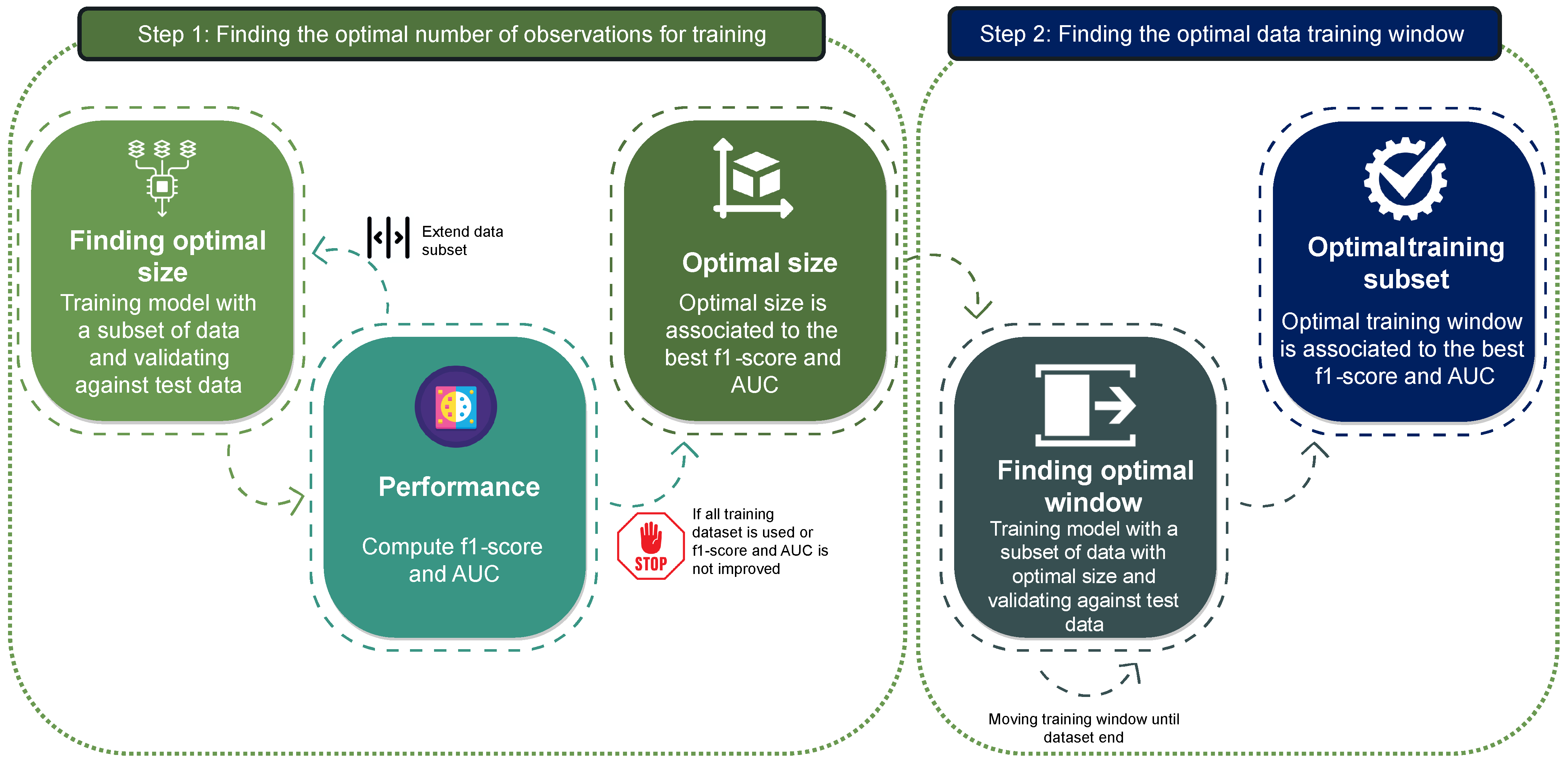
4. Proposed Methodology
4.1. Performance Metrics
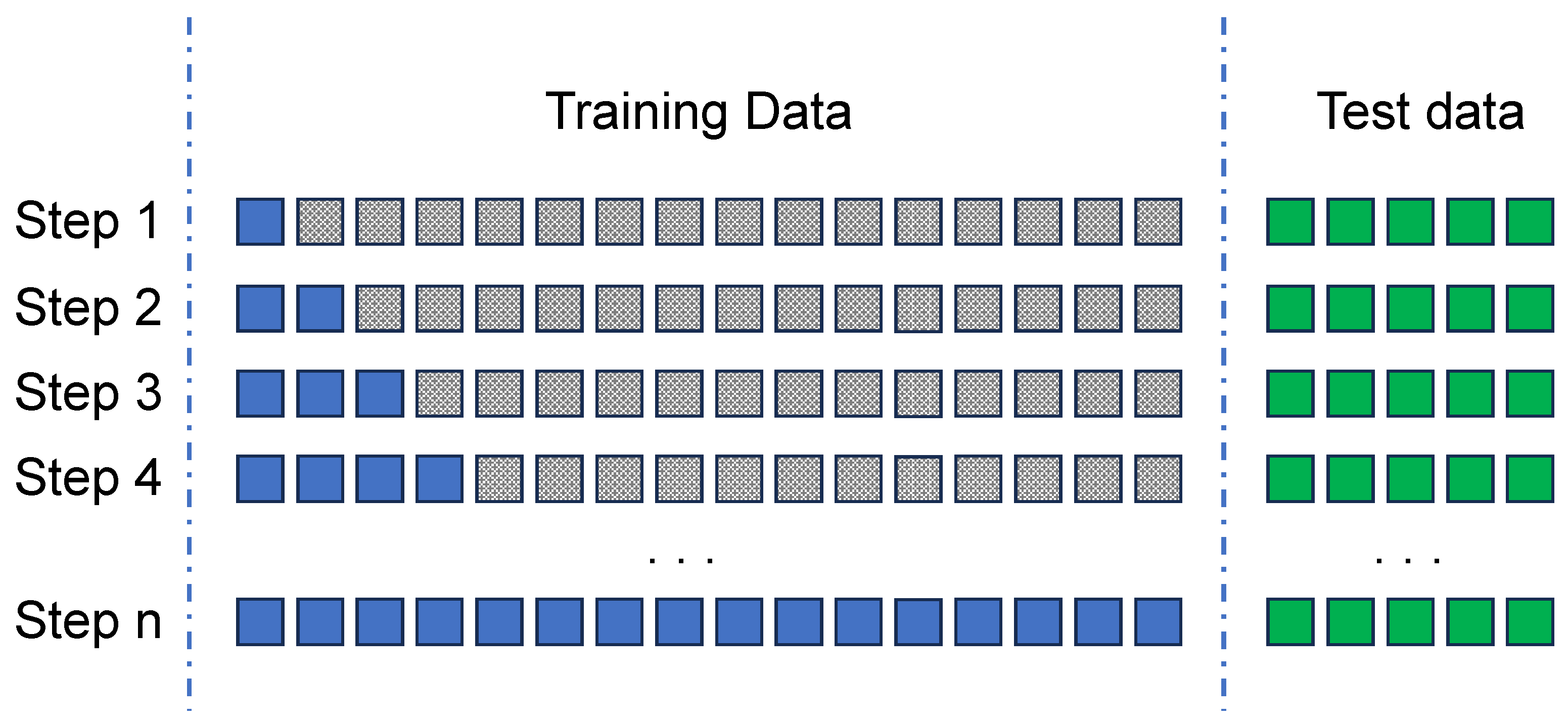
4.2. Optimal Number of Observations for Training
4.2.1. Finding the Best Size for the Training Window
4.2.2. Early Stopping
| Algorithm 1 Step 1: Finding the optimal number of observations for training |
| Require: Training dataset, Test dataset and incremental unit (number or flows/pactkets, hours, days, weeks, …) |
| Ensure: The (pseudo) optimal window size |
| while do |
| if or then |
| else |
| end if |
| if or then |
| end if |
| end while |
4.3. Optimal Data Window Size for Training: A Sliding Window Approach
- Identify the ideal training data window or sequence from the training dataset to maximise model performance. This dataset will be used to train any machine learning model-based NIDS that uses it.
- Analyse the performance of different models trained on each subset of the training set to uncover hidden anomalies in the dataset.
4.3.1. Finding the Optimal Data Training Window
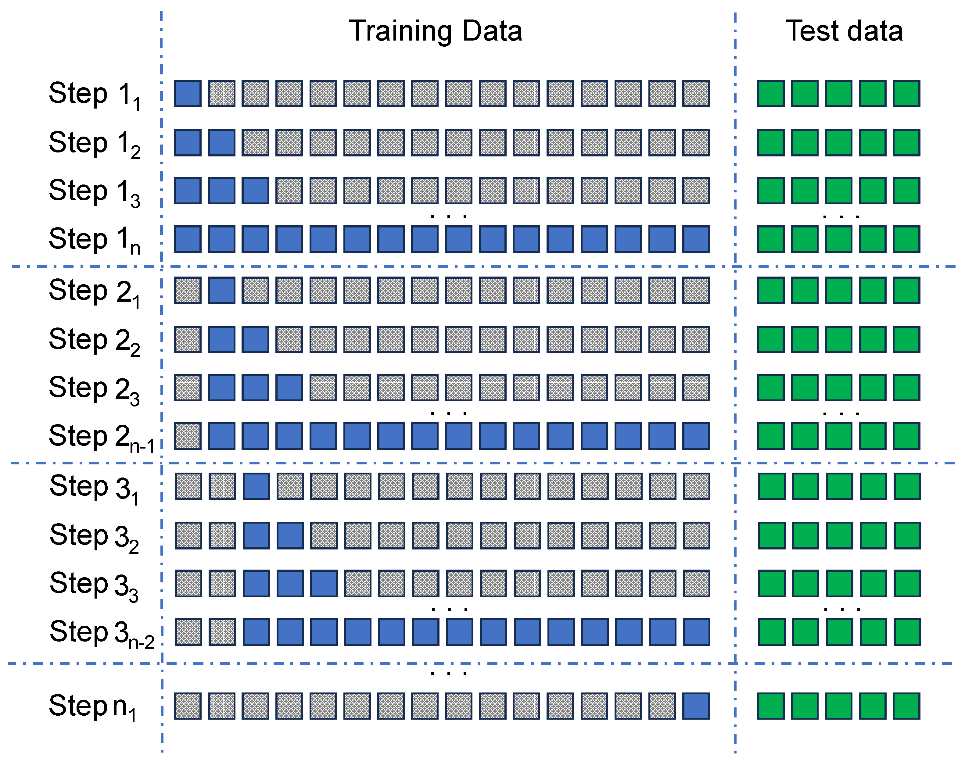
- Step 1: The model is first trained using the training data from the initial 5 days of the dataset. The model is then re-validated against the test data to generate the F1-score and AUC values.
- Step 2: In the second step, the model is trained with the training data obtained from the subsequent 5 days of the dataset (day 1 to day 6), by sliding the window by one day. Afterwards, it is validated against the complete test dataset, and the resulting F1-score and AUC performance indicators are obtained.
- Step n: These steps are repeated for all subsequent iterations (n). The training window is shifted successively until it occupies the final 5 days of the training dataset. The F1-score and AUC are calculated as in other iterations.
4.3.2. Hidden Anomaly Detection
| Algorithm 2 Step 2: Finding the optimal data window for training |
| Require: Training dataset, Test dataset and window size (number or flows/pactkets, hours, days, weeks, …) |
| Ensure: The optimal training window |
| while do |
| if or then |
| end if |
| end while |
4.4. Exhaustive Search for Optimal Window
| Algorithm 3 Exhaustive search for the optimal data training window |
| Require: Training dataset, Test dataset and window size (number or flows/pactkets, hours, days, weeks, …) |
| Ensure: The optimal training window |
| for to n do |
| for to n do |
| if or then |
| end if |
| end for |
| end for |
5. Results
5.1. Description of the Validation Scenario
- Instead of using UGR’16 packets, the data are represented by numerical features derived from the Feature as a Counter method, as explained in Section 3.2.
- Out of the entire UGR’16 dataset that was allocated for training, any observations corresponding to attacks were removed. This was performed in order to create a training dataset that is free of anomalies, which is a requirement for KitNET.
- The state-of-the-art NIDS applied in this experimentation scenario is Kitsune (Section 3.1), although its application is reduced to the use of the Anomaly Detector (KitNET) together with the features extracted from UGR’16.
- The specific configuration parameters for the KitNET model are as follows:
- –
- The maximum size of each autoencoder in the internal ensemble is empirically set to 10 neurons in the hidden layer.
- –
- The number of instances from each scenario’s training dataset used for the initialisation phase of KitNET is empirically set to 2000.
- –
- The proportion of instances from every training dataset scenario used for KitNET’s training sub-phase is set to 70%.
- –
- The proportion of instances used for the KitNET validation sub-phase, therefore, is 30%.
- –
- A uniform value for the threshold or tolerance threshold for anomaly detection has been utilized in all cases—the standard deviation added to the mean of the probabilities detected during the training phase. Values above this threshold are considered anomalous.
- Since we have defined for KitNET 2000 observations for the initialisation phase, the initial window must be at least 2 days long.
- In each iteration, the window for the first step of the methodology is 1 day.
- Instead of using the exhaustive search in order to minimise the computational cost, an early stopping mechanism is implemented based on a total of 10 iterations, which improves neither the F1-score nor the maximum AUC found so far.
5.2. Experiment Results
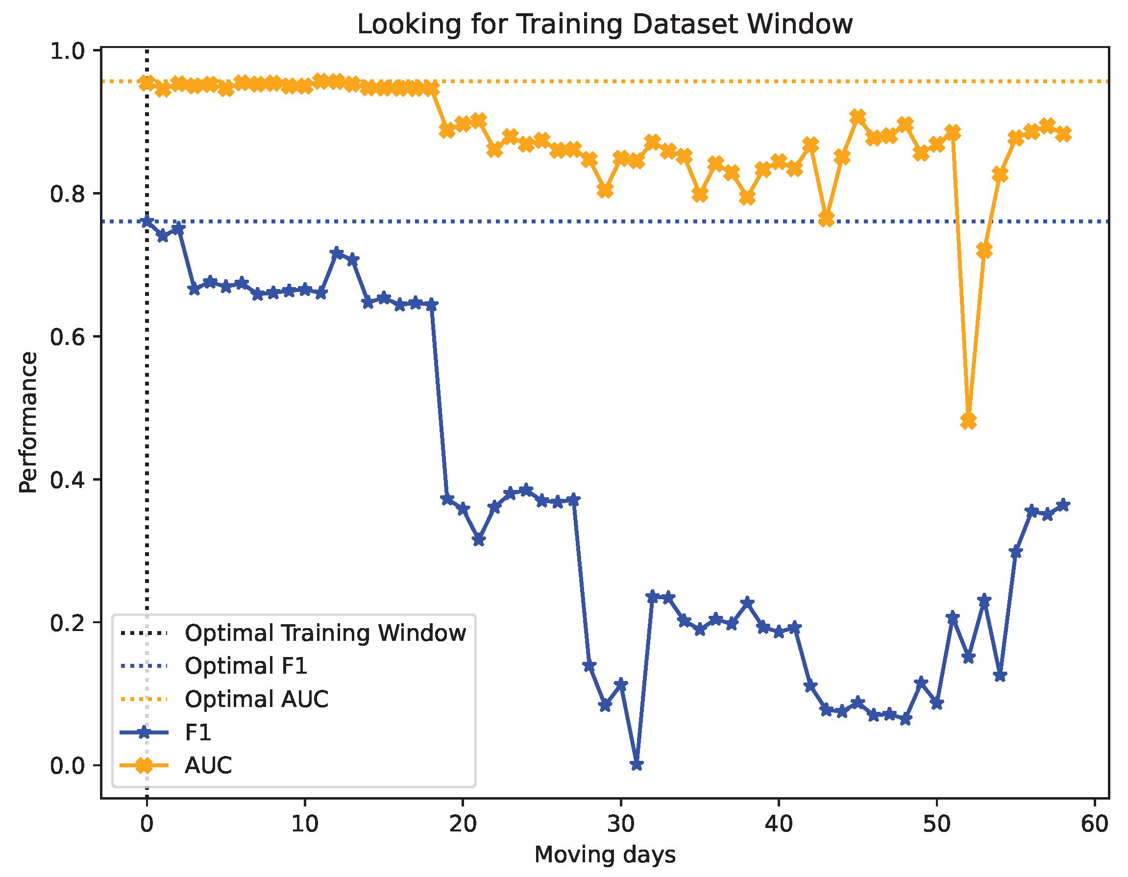
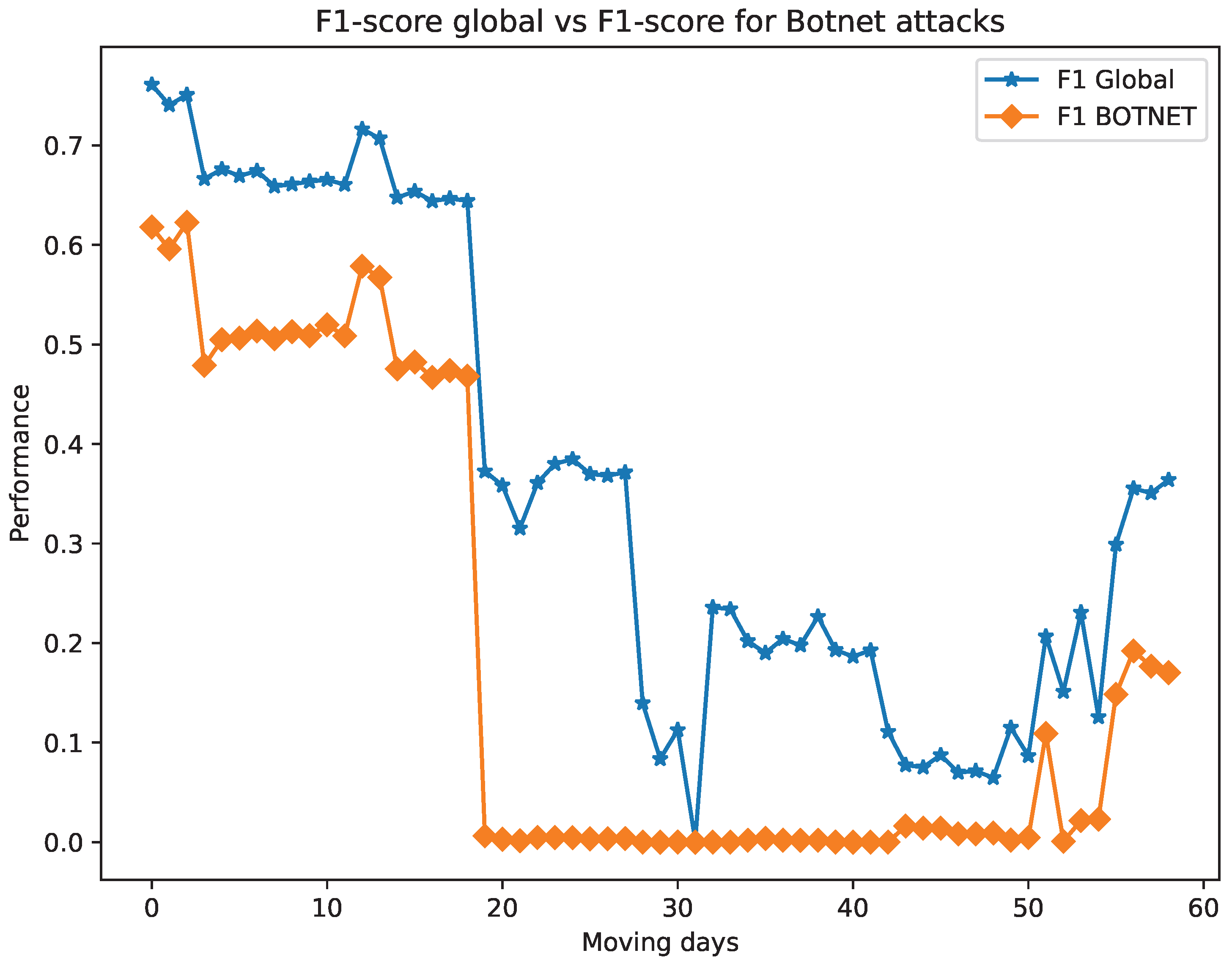
5.2.1. Step 1—Looking for the Window Size
5.2.2. Step 2—Looking for the Optimal Training Window
6. Discussion
6.1. Results on Looking for the Training Window Size
6.2. Results on Looking for the Optimal Training Window
7. Conclusions
Author Contributions
Funding
Institutional Review Board Statement
Informed Consent Statement
Data Availability Statement
Acknowledgments
Conflicts of Interest
References
- Ahmad, Z.; Shahid Khan, A.; Wai Shiang, C.; Abdullah, J.; Ahmad, F. Network intrusion detection system: A systematic study of machine learning and deep learning approaches. Trans. Emerg. Telecommun. Technol. 2021, 32, e4150. [Google Scholar] [CrossRef]
- Liao, H.J.; Richard Lin, C.H.; Lin, Y.C.; Tung, K.Y. Intrusion detection system: A comprehensive review. J. Netw. Comput. Appl. 2013, 36, 16–24. [Google Scholar] [CrossRef]
- Murali, A.; Rao, M. A Survey on Intrusion Detection Approaches. In Proceedings of the 2005 International Conference on Information and Communication Technologies, Karachi, Pakistan, 27–28 August 2005; pp. 233–240. [Google Scholar] [CrossRef]
- Patcha, A.; Park, J.M. An overview of anomaly detection techniques: Existing solutions and latest technological trends. Comput. Netw. 2007, 51, 3448–3470. [Google Scholar] [CrossRef]
- García-Teodoro, P.; Díaz-Verdejo, J.; Maciá-Fernández, G.; Vázquez, E. Anomaly-based network intrusion detection: Techniques, systems and challenges. Comput. Secur. 2009, 28, 18–28. [Google Scholar] [CrossRef]
- Wang, H.; Gu, J.; Wang, S. An effective intrusion detection framework based on SVM with feature augmentation. Knowl.-Based Syst. 2017, 136, 130–139. [Google Scholar] [CrossRef]
- Yeung, D.Y.; Ding, Y. Host-based intrusion detection using dynamic and static behavioral models. Pattern Recognit. 2003, 36, 229–243. [Google Scholar] [CrossRef]
- Mahoney, M.V.; Chan, P.K. Learning nonstationary models of normal network traffic for detecting novel attacks. In Proceedings of the Eighth ACM SIGKDD International Conference on Knowledge Discovery and Data Mining, Edmonton, AB, Canada, 23–26 July 2002; pp. 376–385. [Google Scholar] [CrossRef]
- Mirsky, Y.; Doitshman, T.; Elovici, Y.; Shabtai, A. Kitsune: An Ensemble of Autoencoders for Online Network Intrusion Detection. arXiv 2018, arXiv:1802.09089. [Google Scholar] [CrossRef]
- Li, J.; Manikopoulos, C.; Jorgenson, J.; Ucles, J. HIDE: A Hierarchical Network Intrusion Detection System Using Statistical Preprocessing and Neural Network Classification. In Proceedings of the 2001 IEEE Workshop on Information Assurance and Security, West Point, NY, USA, 5–6 June 2001. [Google Scholar]
- Poojitha, G.; Kumar, K.N.; Reddy, P.J. Intrusion Detection using Artificial Neural Network. In Proceedings of the 2010 Second International Conference on Computing, Communication and Networking Technologies, Karur, India, 29–31 July 2010; pp. 1–7. [Google Scholar] [CrossRef]
- Ghosh, A.K.; Michael, C.; Schatz, M. A Real-Time Intrusion Detection System Based on Learning Program Behavior. In Recent Advances in Intrusion Detection, Proceedings of the Third International Workshop, RAID 2000, Toulouse, France, 2–4 October 2000; Debar, H., Mé, L., Wu, S.F., Eds.; Lecture Notes in Computer Science; Springer: Berlin/Heidelberg, Germany, 2000; pp. 93–109. [Google Scholar] [CrossRef]
- Ullah, S.; Ahmad, J.; Khan, M.A.; Alkhammash, E.H.; Hadjouni, M.; Ghadi, Y.Y.; Saeed, F.; Pitropakis, N. A New Intrusion Detection System for the Internet of Things via Deep Convolutional Neural Network and Feature Engineering. Sensors 2022, 22, 3607. [Google Scholar] [CrossRef]
- Banaamah, A.M.; Ahmad, I. Intrusion Detection in IoT Using Deep Learning. Sensors 2022, 22, 8417. [Google Scholar] [CrossRef]
- Ren, Y.; Feng, K.; Hu, F.; Chen, L.; Chen, Y. A Lightweight Unsupervised Intrusion Detection Model Based on Variational Auto-Encoder. Sensors 2023, 23, 8407. [Google Scholar] [CrossRef]
- Kotecha, K.; Verma, R.; Rao, P.V.; Prasad, P.; Mishra, V.K.; Badal, T.; Jain, D.; Garg, D.; Sharma, S. Enhanced Network Intrusion Detection System. Sensors 2021, 21, 7835. [Google Scholar] [CrossRef] [PubMed]
- Chandola, V.; Eilertson, E.; Ertoz, L.; Simon, G.; Kumar, V. Minds: Architecture & Design. In Data Warehousing and Data Mining Techniques for Cyber Security; Singhal, A., Ed.; Advances in Information Security; Springer: Boston, MA, USA, 2007; pp. 83–107. [Google Scholar] [CrossRef]
- Ahmed, M.; Naser Mahmood, A.; Hu, J. A survey of network anomaly detection techniques. J. Netw. Comput. Appl. 2016, 60, 19–31. [Google Scholar] [CrossRef]
- García Fuentes, M.N. Multivariate Statistical Network Monitoring for Network Security Based on Principal Component Analysis; Universidad de Granada: Granada, Spain, 2021. [Google Scholar]
- Medina-Arco, J.G.; Magán-Carrión, R.; Rodríguez-Gómez, R.A. Exploring Hidden Anomalies in UGR’16 Network Dataset with Kitsune. In Flexible Query Answering Systems, Proceedings of the 15th International Conference, FQAS 2023, Mallorca, Spain, 5–7 September 2023; Larsen, H.L., Martin-Bautista, M.J., Ruiz, M.D., Andreasen, T., Bordogna, G., De Tré, G., Eds.; Lecture Notes in Computer Science; Springer: Cham, Switzerland, 2023; pp. 194–205. [Google Scholar] [CrossRef]
- Butun, I.; Österberg, P.; Song, H. Security of the Internet of Things: Vulnerabilities, Attacks, and Countermeasures. IEEE Commun. Surv. Tutorials 2020, 22, 616–644. [Google Scholar] [CrossRef]
- Antonakakis, M.; April, T.; Bailey, M.; Bernhard, M.; Bursztein, E.; Cochran, J.; Durumeric, Z.; Halderman, J.A.; Invernizzi, L.; Kallitsis, M.; et al. Understanding the Mirai Botnet. In Proceedings of the 26th USENIX Security Symposium, Vancouver, BC, Canada, 16–18 August 2017; pp. 1093–1110. [Google Scholar]
- De Keersmaeker, F.; Cao, Y.; Ndonda, G.K.; Sadre, R. A Survey of Public IoT Datasets for Network Security Research. IEEE Commun. Surv. Tutor. 2023, 25, 1808–1840. [Google Scholar] [CrossRef]
- Hasan, M.; Islam, M.M.; Zarif, M.I.I.; Hashem, M.M.A. Attack and anomaly detection in IoT sensors in IoT sites using machine learning approaches. Internet Things 2019, 7, 100059. [Google Scholar] [CrossRef]
- Camacho, J.; Wasielewska, K.; Espinosa, P.; Fuentes-García, M. Quality In/Quality Out: Data quality more relevant than model choice in anomaly detection with the UGR’16. In Proceedings of the NOMS 2023—2023 IEEE/IFIP Network Operations and Management Symposium, Miami, FL, USA, 8–12 May 2023; pp. 1–5. [Google Scholar] [CrossRef]
- Lippmann, R.; Haines, J.W.; Fried, D.J.; Korba, J.; Das, K. The 1999 DARPA off-line intrusion detection evaluation. Comput. Netw. 2000, 34, 579–595. [Google Scholar] [CrossRef]
- Salvatore Stolfo, W.F. KDD Cup 1999 Data; UCI Machine Learning Repository, 1999. [Google Scholar] [CrossRef]
- Tavallaee, M.; Bagheri, E.; Lu, W.; Ghorbani, A.A. A detailed analysis of the KDD CUP 99 data set. In Proceedings of the 2009 IEEE Symposium on Computational Intelligence for Security and Defense Applications, Ottawa, ON, Canada, 8–10 July 2009; pp. 1–6. [Google Scholar] [CrossRef]
- Biglar Beigi, E.; Hadian Jazi, H.; Stakhanova, N.; Ghorbani, A.A. Towards effective feature selection in machine learning-based botnet detection approaches. In Proceedings of the 2014 IEEE Conference on Communications and Network Security, San Francisco, CA, USA, 29–31 October 2014; pp. 247–255. [Google Scholar] [CrossRef]
- Moustafa, N.; Slay, J. UNSW-NB15: A comprehensive data set for network intrusion detection systems (UNSW-NB15 network data set). In Proceedings of the 2015 Military Communications and Information Systems Conference (MilCIS), Canberra, ACT, Australia, 10–12 November 2015; pp. 1–6. [Google Scholar] [CrossRef]
- Maciá-Fernández, G.; Camacho, J.; Magán-Carrión, R.; García-Teodoro, P.; Therón, R. UGR‘16: A new dataset for the evaluation of cyclostationarity-based network IDSs. Comput. Secur. 2018, 73, 411–424. [Google Scholar] [CrossRef]
- Sharafaldin, I.; Habibi Lashkari, A.; Ghorbani, A.A. Toward Generating a New Intrusion Detection Dataset and Intrusion Traffic Characterization. In Proceedings of the 4th International Conference on Information Systems Security and Privacy, Funchal, Madeira, Portugal, 22–24 January 2018; pp. 108–116. [Google Scholar] [CrossRef]
- Canadian Institute for Cybersecurity. CSE-CIC-IDS2018. 2018. Available online: https://www.unb.ca/cic/datasets/ids-2018.html (accessed on 30 November 2023).
- Sarhan, M.; Layeghy, S.; Moustafa, N.; Portmann, M. NetFlow Datasets for Machine Learning-Based Network Intrusion Detection Systems. In Big Data Technologies and Applications, Proceedings of the 10th EAI International Conference, BDTA 2020, and 13th EAI International Conference on Wireless Internet, WiCON 2020, Virtual Event, 11 December 2020; Deze, Z., Huang, H., Hou, R., Rho, S., Chilamkurti, N., Eds.; Lecture Notes of the Institute for Computer Sciences, Social Informatics and Telecommunications Engineering; Springer: Cham, Switzerland, 2021; pp. 117–135. [Google Scholar] [CrossRef]
- Ring, M.; Wunderlich, S.; Scheuring, D.; Landes, D.; Hotho, A. A Survey of Network-based Intrusion Detection Data Sets. Comput. Secur. 2019, 86, 147–167. [Google Scholar] [CrossRef]
- Thomas, C.; Sharma, V.; Balakrishnan, N. Usefulness of DARPA dataset for intrusion detection system evaluation. In Proceedings of the Data Mining, Intrusion Detection, Information Assurance, and Data Networks Security, Orlando, FL, USA, 17–18 March 2008; Volume 6973, pp. 164–171. [Google Scholar] [CrossRef]
- McHugh, J. Testing Intrusion detection systems: A critique of the 1998 and 1999 DARPA intrusion detection system evaluations as performed by Lincoln Laboratory. ACM Trans. Inf. Syst. Secur. 2000, 3, 262–294. [Google Scholar] [CrossRef]
- Chaabouni, N.; Mosbah, M.; Zemmari, A.; Sauvignac, C.; Faruki, P. Network Intrusion Detection for IoT Security Based on Learning Techniques. IEEE Commun. Surv. Tutor. 2019, 21, 2671–2701. [Google Scholar] [CrossRef]
- Sabahi, F.; Movaghar, A. Intrusion Detection: A Survey. In Proceedings of the 2008 Third International Conference on Systems and Networks Communications, Sliema, Malta, 26–31 October 2008; pp. 23–26. [Google Scholar] [CrossRef]
- Song, J.; Takakura, H.; Okabe, Y.; Eto, M.; Inoue, D.; Nakao, K. Statistical analysis of honeypot data and building of Kyoto 2006+ dataset for NIDS evaluation. In Proceedings of the First Workshop on Building Analysis Datasets and Gathering Experience Returns for Security, BADGERS ’11, Salzburg, Austria, 10 April 2011; pp. 29–36. [Google Scholar] [CrossRef]
- Saad, S.; Traore, I.; Ghorbani, A.; Sayed, B.; Zhao, D.; Lu, W.; Felix, J.; Hakimian, P. Detecting P2P botnets through network behavior analysis and machine learning. In Proceedings of the 2011 Ninth Annual International Conference on Privacy, Security and Trust, Montreal, QC, Canada, 19–21 July 2011; pp. 174–180. [Google Scholar] [CrossRef]
- Shiravi, A.; Shiravi, H.; Tavallaee, M.; Ghorbani, A.A. Toward developing a systematic approach to generate benchmark datasets for intrusion detection. Comput. Secur. 2012, 31, 357–374. [Google Scholar] [CrossRef]
- García, S.; Grill, M.; Stiborek, J.; Zunino, A. An empirical comparison of botnet detection methods. Comput. Secur. 2014, 45, 100–123. [Google Scholar] [CrossRef]
- Aviv, A.J.; Haeberlen, A. Challenges in experimenting with botnet detection systems. In Proceedings of the 4th Conference on Cyber Security Experimentation and Test, San Francisco, CA, USA, 8 August 2011; CSET’11. p. 6. [Google Scholar]
- Koroniotis, N.; Moustafa, N.; Sitnikova, E.; Turnbull, B. Towards the Development of Realistic Botnet Dataset in the Internet of Things for Network Forensic Analytics: Bot-IoT Dataset. arXiv 2018, arXiv:1811.00701. [Google Scholar] [CrossRef]
- Moustafa, N. ToN_IoT Datasets; IEEE: Piscataway, NJ, USA, 2019. [Google Scholar] [CrossRef]
- Northcutt, C.G.; Athalye, A.; Mueller, J. Pervasive Label Errors in Test Sets Destabilize Machine Learning Benchmarks. arXiv 2021, arXiv:2103.14749. [Google Scholar] [CrossRef]
- Kremer, J.; Sha, F.; Igel, C. Robust Active Label Correction. In Proceedings of the Twenty-First International Conference on Artificial Intelligence and Statistics. PMLR, Playa Blanca, Spain, 9–11 April 2018; pp. 308–316. [Google Scholar]
- Zhang, J.; Sheng, V.S.; Li, T.; Wu, X. Improving Crowdsourced Label Quality Using Noise Correction. IEEE Trans. Neural Netw. Learn. Syst. 2018, 29, 1675–1688. [Google Scholar] [CrossRef] [PubMed]
- Cabrera, G.F.; Miller, C.J.; Schneider, J. Systematic Labeling Bias: De-biasing Where Everyone is Wrong. In Proceedings of the 2014 22nd International Conference on Pattern Recognition, Stockholm, Sweden, 24–28 August 2014; pp. 4417–4422. [Google Scholar] [CrossRef]
- Natarajan, N.; Dhillon, I.S.; Ravikumar, P.K.; Tewari, A. Learning with Noisy Labels. In Advances in Neural Information Processing Systems; Curran Associates, Inc.: Red Hook, NY, USA, 2013; Volume 26. [Google Scholar]
- Patrini, G.; Rozza, A.; Menon, A.; Nock, R.; Qu, L. Making Deep Neural Networks Robust to Label Noise: A Loss Correction Approach. arXiv 2017, arXiv:1609.03683. [Google Scholar] [CrossRef]
- Wei, J.; Zhu, Z.; Cheng, H.; Liu, T.; Niu, G.; Liu, Y. Learning with Noisy Labels Revisited: A Study Using Real-World Human Annotations. arXiv 2022, arXiv:2110.12088. [Google Scholar] [CrossRef]
- Northcutt, C.; Jiang, L.; Chuang, I. Confident Learning: Estimating Uncertainty in Dataset Labels. J. Artif. Intell. Res. 2021, 70, 1373–1411. [Google Scholar] [CrossRef]
- Müller, N.M.; Markert, K. Identifying Mislabeled Instances in Classification Datasets. In Proceedings of the 2019 International Joint Conference on Neural Networks (IJCNN), Budapest, Hungary, 14–19 July 2019; pp. 1–8. [Google Scholar] [CrossRef]
- Hao, D.; Zhang, L.; Sumkin, J.; Mohamed, A.; Wu, S. Inaccurate Labels in Weakly-Supervised Deep Learning: Automatic Identification and Correction and Their Impact on Classification Performance. IEEE J. Biomed. Health Inform. 2020, 24, 2701–2710. [Google Scholar] [CrossRef]
- Bekker, A.J.; Goldberger, J. Training deep neural-networks based on unreliable labels. In Proceedings of the 2016 IEEE International Conference on Acoustics, Speech and Signal Processing (ICASSP), Shanghai, China, 20–25 March 2016; pp. 2682–2686. [Google Scholar] [CrossRef]
- Cordero, C.G.; Vasilomanolakis, E.; Wainakh, A.; Mühlhäuser, M.; Nadjm-Tehrani, S. On Generating Network Traffic Datasets with Synthetic Attacks for Intrusion Detection. ACM Trans. Priv. Secur. 2021, 24, 1–39. [Google Scholar] [CrossRef]
- Guerra, J.L.; Catania, C.; Veas, E. Datasets are not enough: Challenges in labeling network traffic. Comput. Secur. 2022, 120, 102810. [Google Scholar] [CrossRef]
- Soukup, D.; Tisovčík, P.; Hynek, K.; Čejka, T. Towards Evaluating Quality of Datasets for Network Traffic Domain. In Proceedings of the 2021 17th International Conference on Network and Service Management (CNSM), Izmir, Turkey, 25–29 October 2021; pp. 264–268. [Google Scholar] [CrossRef]
- Packet++. 2023. Available online: https://github.com/seladb/PcapPlusPlus (accessed on 30 November 2023).
- Mirsky, Y. KitNET. 2018. Available online: https://github.com/ymirsky/KitNET-py (accessed on 30 November 2023).
- Magán-Carrión, R.; Urda, D.; Díaz-Cano, I.; Dorronsoro, B. Towards a Reliable Comparison and Evaluation of Network Intrusion Detection Systems Based on Machine Learning Approaches. Appl. Sci. 2020, 10, 1775. [Google Scholar] [CrossRef]
- Camacho, J.; Maciá-Fernández, G.; Díaz-Verdejo, J.; García-Teodoro, P. Tackling the Big Data 4 vs for anomaly detection. In Proceedings of the 2014 IEEE Conference on Computer Communications Workshops (INFOCOM WKSHPS), Toronto, ON, Canada, 27 April–2 May 2014; pp. 500–505. [Google Scholar] [CrossRef]
- Camacho, J. FCParser. 2022. Available online: https://github.com/josecamachop/FCParser (accessed on 20 November 2023).
- Lipton, Z.C.; Elkan, C.; Naryanaswamy, B. Optimal Thresholding of Classifiers to Maximize F1 Measure. In Proceedings of the Machine Learning and Knowledge Discovery in Databases, Nancy, France, 15–19 September 2014; Calders, T., Esposito, F., Hüllermeier, E., Meo, R., Eds.; Lecture Notes in Computer Science. Springer: Berlin/Heidelberg, Germany, 2014; pp. 225–239. [Google Scholar] [CrossRef]
- Powers, D.M.W. Evaluation: From precision, recall and F-measure to ROC, informedness, markedness and correlation. arXiv 2020, arXiv:2010.16061. [Google Scholar] [CrossRef]
- Van, N.T.; Thinh, T.N.; Sach, L.T. A Combination of Temporal Sequence Learning and Data Description for Anomaly-based NIDS. Int. J. Netw. Secur. Its Appl. 2019, 11, 89–100. [Google Scholar] [CrossRef]
- Prechelt, L. Early Stopping—But When? In Neural Networks: Tricks of the Trade; Orr, G.B., Müller, K.R., Eds.; Lecture Notes in Computer Science; Springer: Berlin/Heidelberg, Germany, 1998; pp. 55–69. [Google Scholar] [CrossRef]


| Dataset | Availability | Collected Data | Labeled | Type | Duration * | Size ** | Year | Freshness | Balanced |
|---|---|---|---|---|---|---|---|---|---|
| DARPA [26] | Public | packets | yes | synthetic | 7 weeks | 6.5TB | 1998–1999 | questioned | no |
| NSL-KDD [27] | Public | features | yes | synthetic | N.S. | 5M o. | 1998–1999 | questioned | yes |
| Kyoto 2006+ [28] | Public | features | yes | real | 9 years | 93M o. | 2006–2015 | yes | yes |
| Botnet [29] | Public | packets | yes | synthetic | N.S. | 14GB p. | 2010–2014 | yes | yes |
| UNSW-NB15 [30] | Public | features | yes | synthetic | 31 hours | 2.5M o. | 2015 | yes | no |
| UGR’16 [31] | Public | flows | yes | real | 6 months | 17B f. | 2016 | yes | no |
| CICIDS2017 [32] | Protected | flows | yes | synthetic | 5 days | 3.1M f. | 2017 | yes | no |
| IDS2018 [33] | Protected | features | yes | synthetic | 10 days | 1M o. | 2018 | yes | no |
| NF-UQ-NIDS [34] | Public | flows | yes | synthetic | N.S. | 12M f. | 2021 | yes | no |
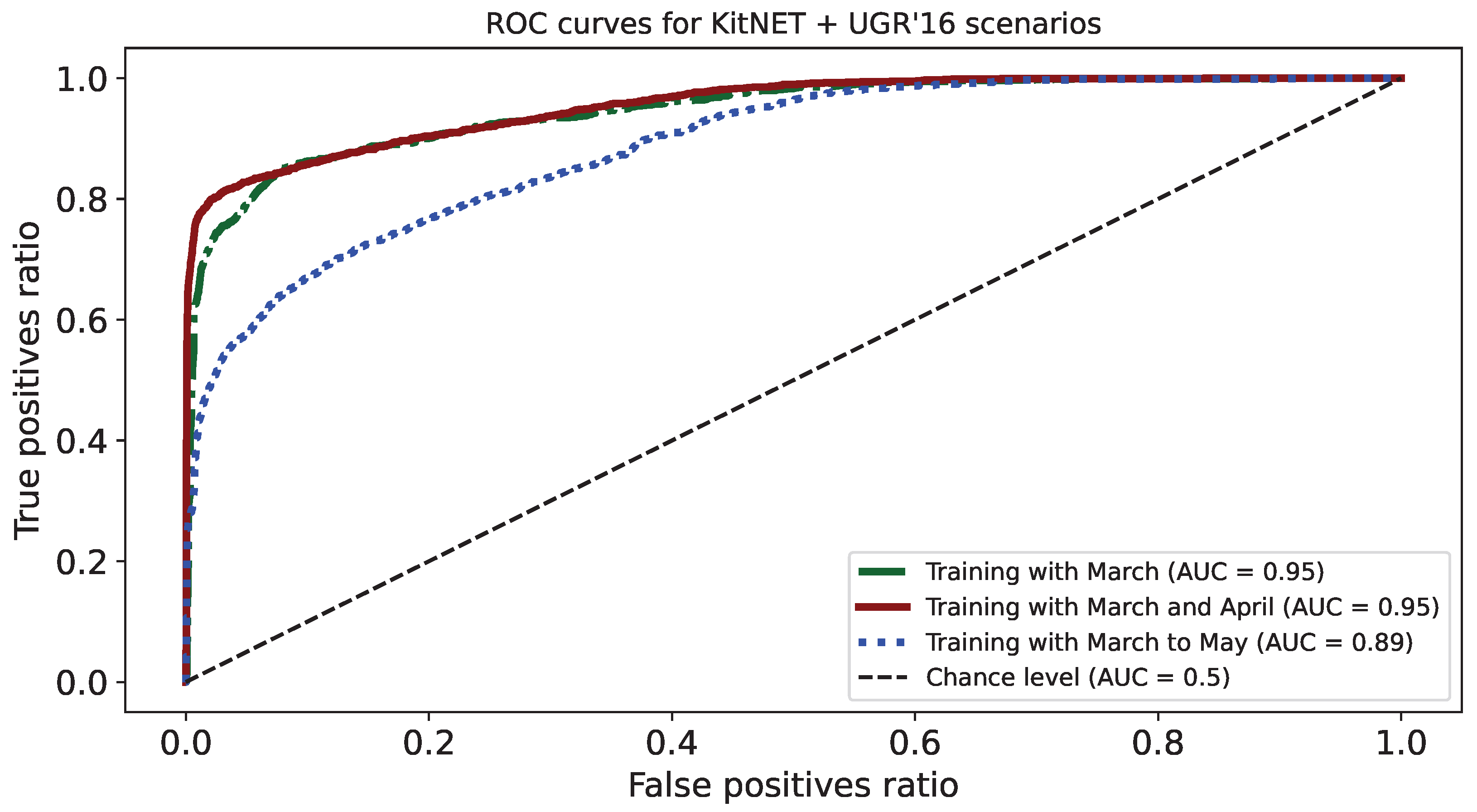
| Scenario | Training Data * | Class | Precision | Recall | F1-Measure | Accuracy |
|---|---|---|---|---|---|---|
| Scenario 1 | March | Normal | 0.99 | 1 | 0.99 | 0.97 |
| Anomalous | 0.75 | 0.17 | 0.27 | |||
| Scenario 2 | March to April | Normal | 0.98 | 1 | 0.99 | 0.99 |
| Anomalous | 0.9 | 0.66 | 0.76 | |||
| Scenario 3 | March to May | Normal | 0.98 | 1 | 0.99 | 0.98 |
| Anomalous | 0.87 | 0.23 | 0.36 |
| Attack | Scenario 1 | Scenario 2 | Scenario 3 |
|---|---|---|---|
| DOS | 34% | 64% | 56% |
| SCAN11 | 1% | 1% | 1% |
| SCAN44 | 51% | 72% | 57% |
| BOTNET | 4% | 74% | 1% |
| UDPSCAN | 0% | 0% | 0% |
| Total | 16% | 65% | 22% |
Disclaimer/Publisher’s Note: The statements, opinions and data contained in all publications are solely those of the individual author(s) and contributor(s) and not of MDPI and/or the editor(s). MDPI and/or the editor(s) disclaim responsibility for any injury to people or property resulting from any ideas, methods, instructions or products referred to in the content. |
© 2024 by the authors. Licensee MDPI, Basel, Switzerland. This article is an open access article distributed under the terms and conditions of the Creative Commons Attribution (CC BY) license (https://creativecommons.org/licenses/by/4.0/).
Share and Cite
Medina-Arco, J.G.; Magán-Carrión, R.; Rodríguez-Gómez, R.A.; García-Teodoro, P. Methodology for the Detection of Contaminated Training Datasets for Machine Learning-Based Network Intrusion-Detection Systems. Sensors 2024, 24, 479. https://doi.org/10.3390/s24020479
Medina-Arco JG, Magán-Carrión R, Rodríguez-Gómez RA, García-Teodoro P. Methodology for the Detection of Contaminated Training Datasets for Machine Learning-Based Network Intrusion-Detection Systems. Sensors. 2024; 24(2):479. https://doi.org/10.3390/s24020479
Chicago/Turabian StyleMedina-Arco, Joaquín Gaspar, Roberto Magán-Carrión, Rafael Alejandro Rodríguez-Gómez, and Pedro García-Teodoro. 2024. "Methodology for the Detection of Contaminated Training Datasets for Machine Learning-Based Network Intrusion-Detection Systems" Sensors 24, no. 2: 479. https://doi.org/10.3390/s24020479
APA StyleMedina-Arco, J. G., Magán-Carrión, R., Rodríguez-Gómez, R. A., & García-Teodoro, P. (2024). Methodology for the Detection of Contaminated Training Datasets for Machine Learning-Based Network Intrusion-Detection Systems. Sensors, 24(2), 479. https://doi.org/10.3390/s24020479