
Phase Noise Analysis of Time Transfer over White Rabbit-Network Based Optical Fibre Links


Abstract
1. Introduction
2. Literature Review and Background
2.1. White Rabbit Technology
2.2. Phase Noise
2.3. Phase Noise in White Rabbit Systems
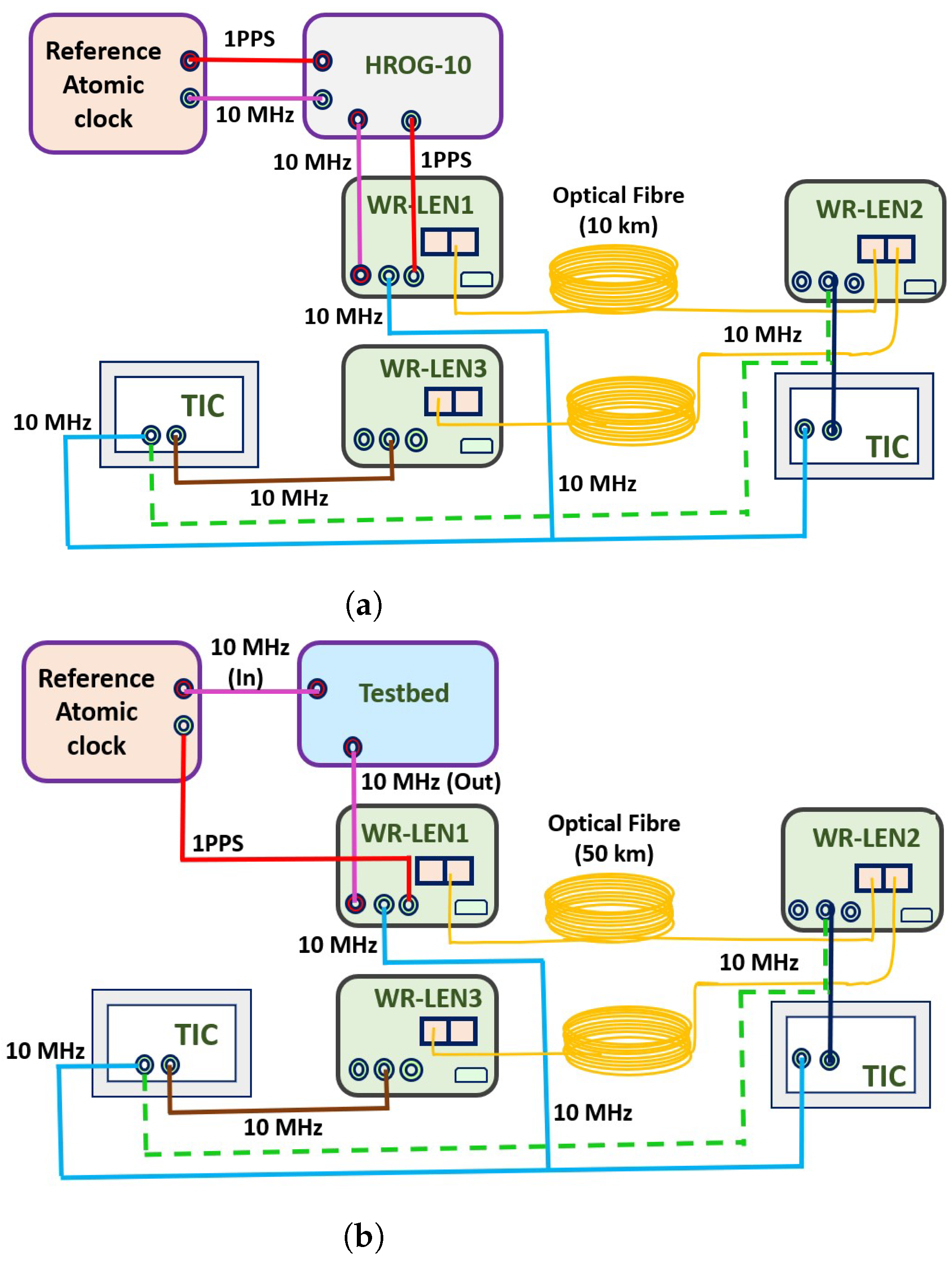
3. Experimental Setup for Phase Noise Measurements
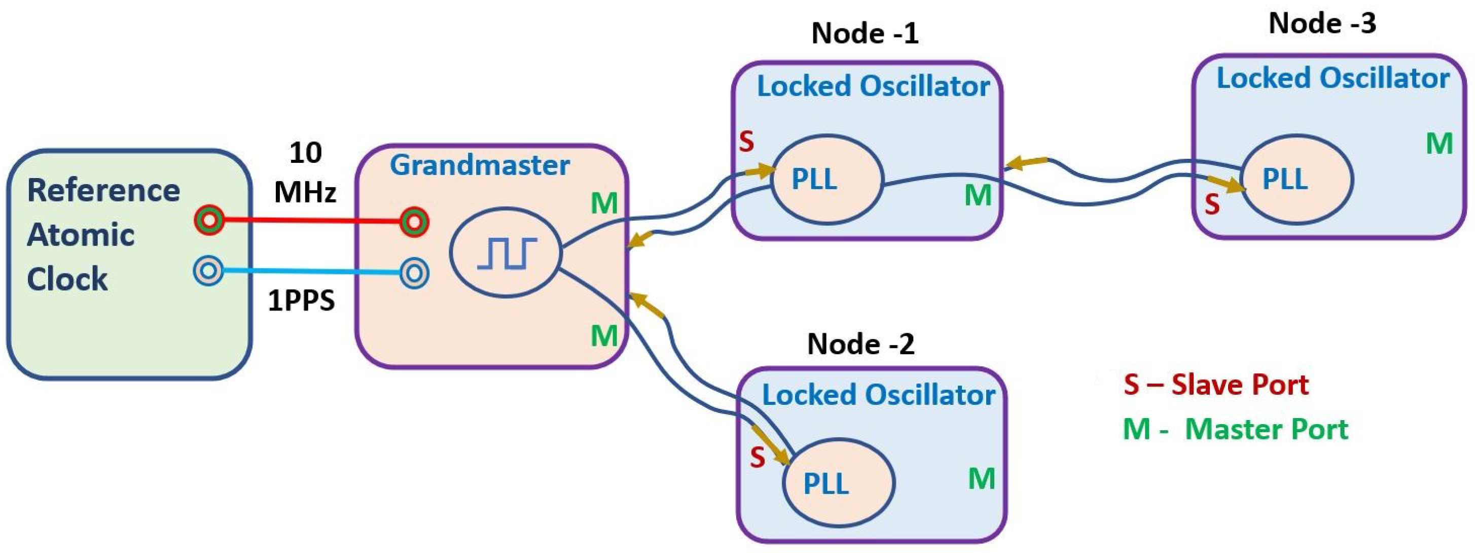
- Grandmaster (GM): In this mode, external reference signals from a highly stable reference clock are required to lock the inbuilt oscillator of the WRLEN with reference clock signals. In the GM mode, both ports of the WRLEN work as masters.
- Master: In this mode, no external reference signals are needed, and the WRLEN’s inbuilt oscillator runs freely. Both ports of the WRLEN work as masters in this mode.
- Slave: In this mode, no external reference signals are needed, and one port of the WRLEN acts as the slave while the other acts as the master. In the present study, in ‘Slave’ mode, the first port of the WRLEN acts as the slave and the second port as the master, as shown in Figure 2a.
3.1. Data Collection and Processing
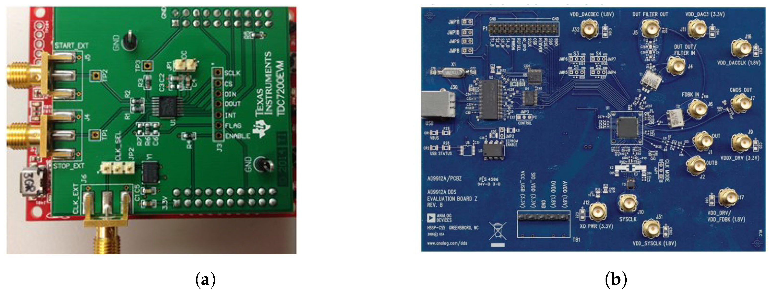
3.2. Testbed Components, Design, and Features
4. Phase Noise Modelling: Statistical Distribution
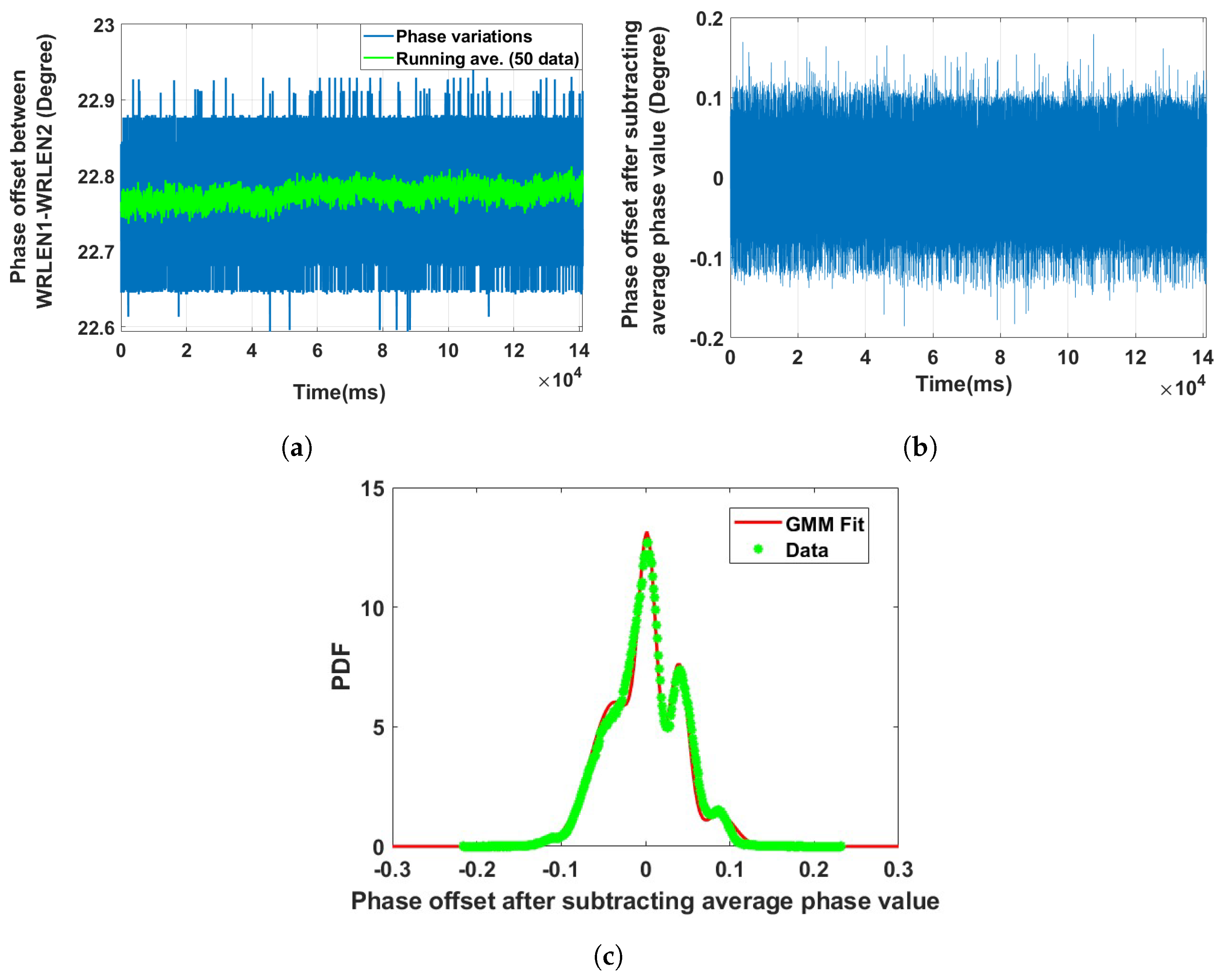
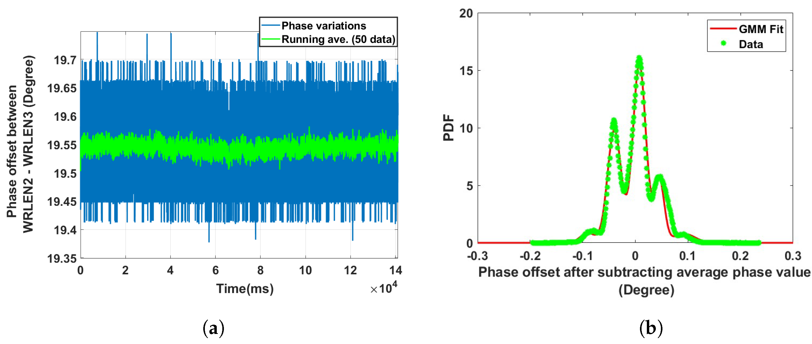
4.1. Phase Noise Distribution Analysis for Experimental Setup A with HROG-10
4.1.1. Data Collection with Gate Time: ms
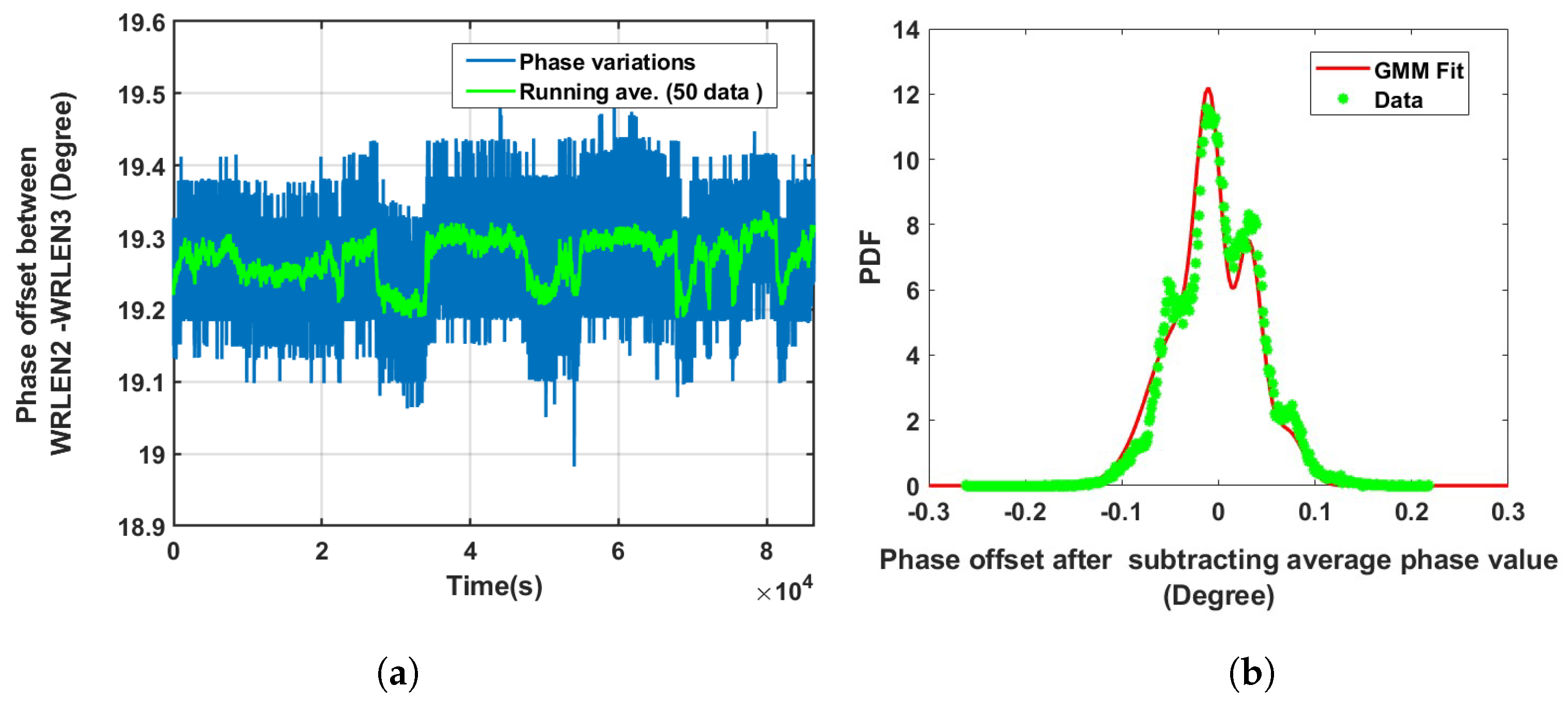
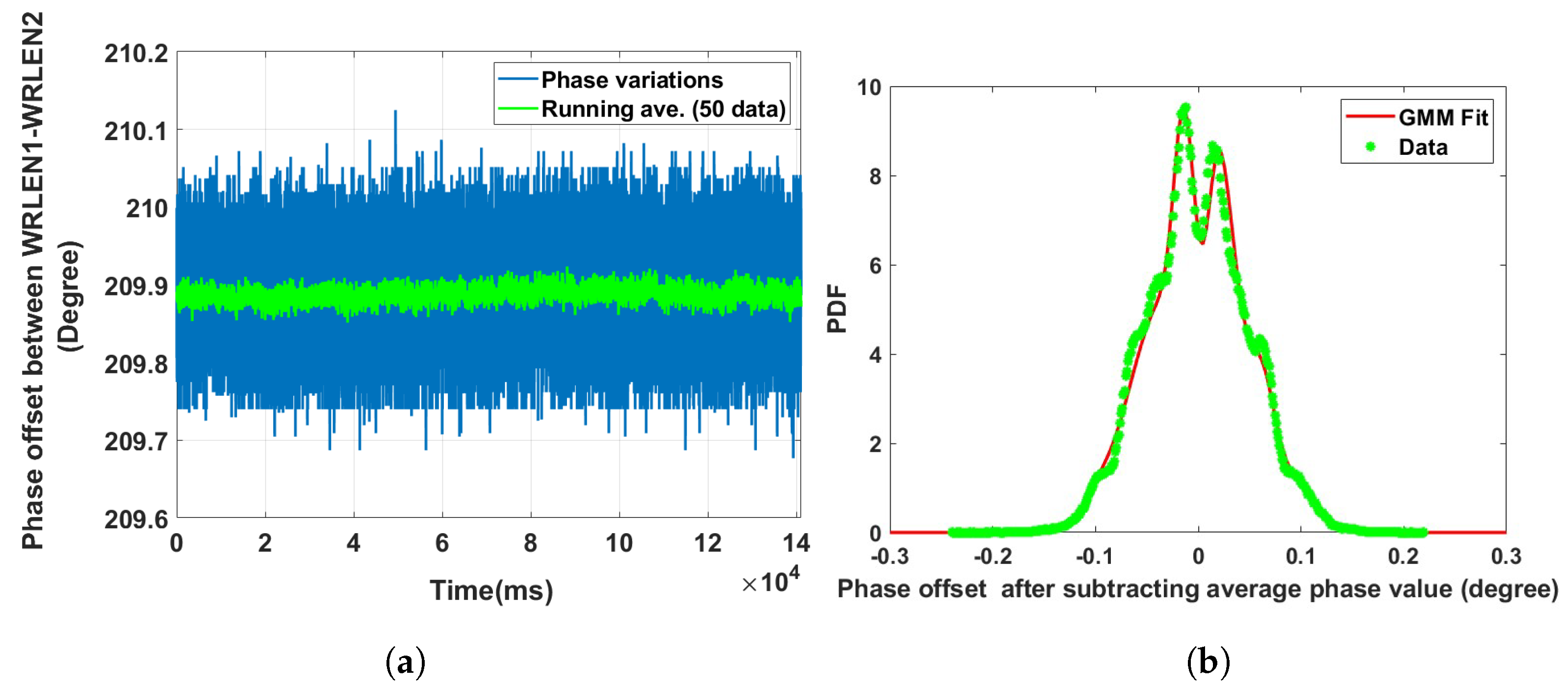
4.1.2. Data Collection with Gate Time: s
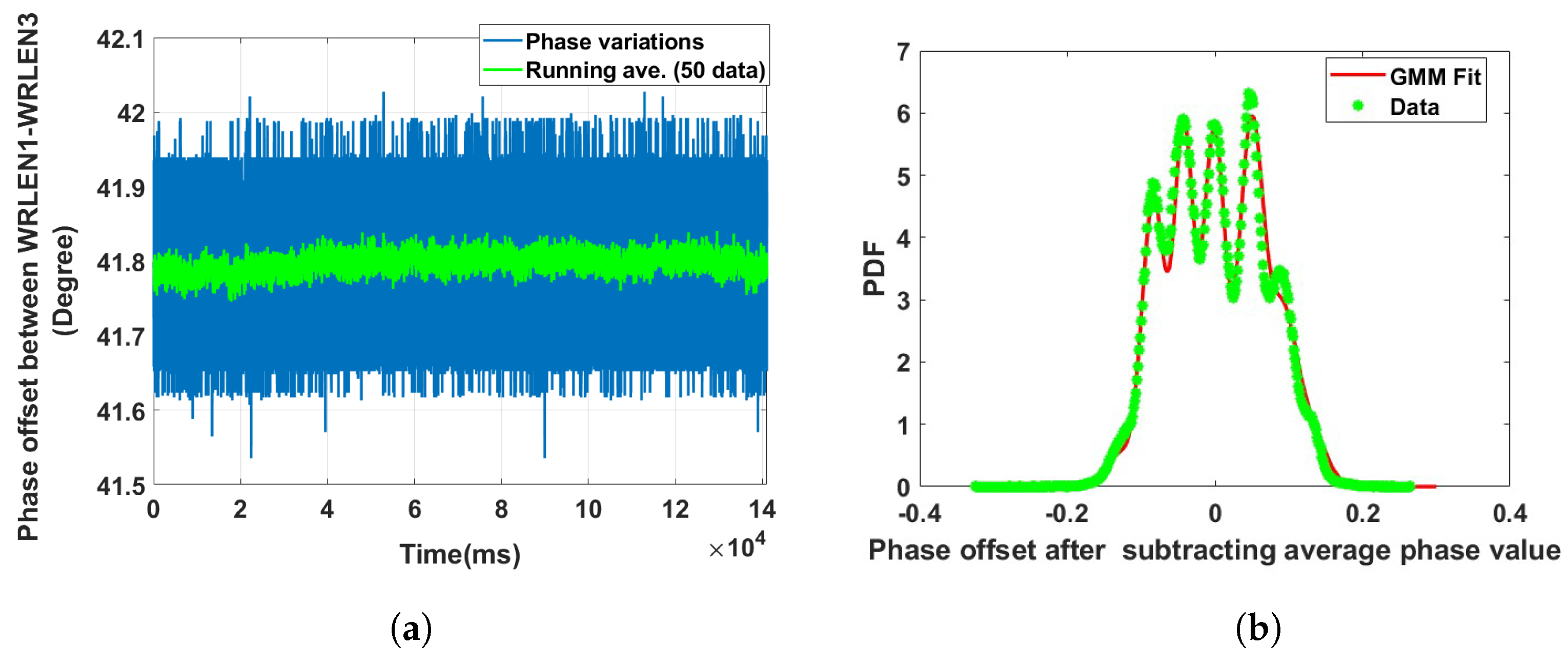
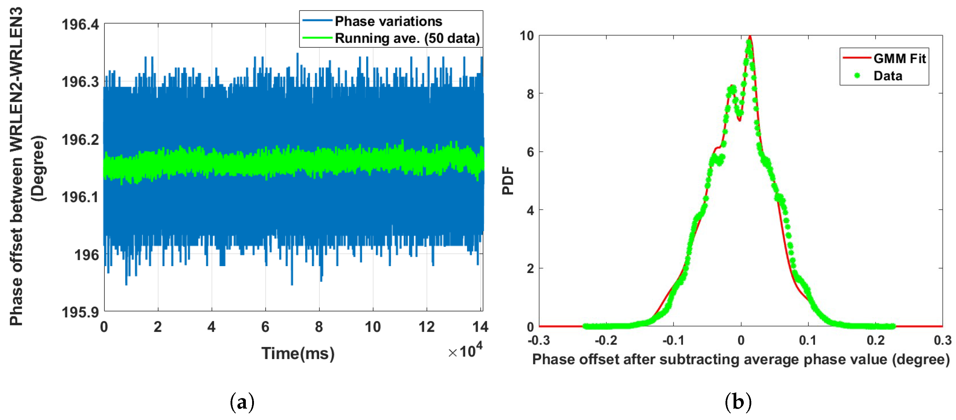
4.2. Phase Noise Distribution Analysis for Experimental Setup B with the Testbed
Data Collection with Gate Time: ms
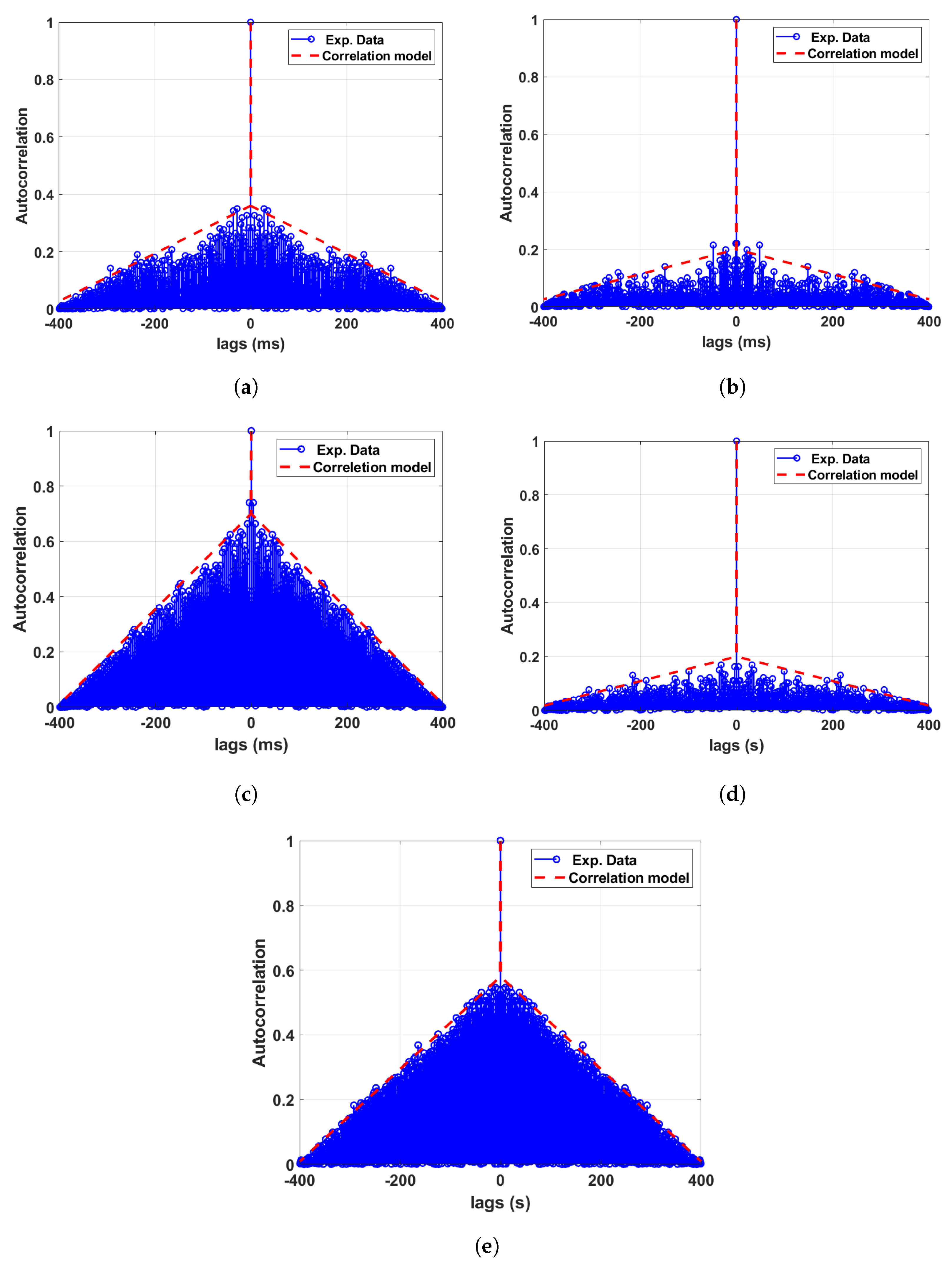
5. Phase Noise Modelling: Autocorrelation
5.1. ACF of the Phase Noise for Test Setup A with HROG-10
5.2. ACF of the Phase Noise for Test Setup B with the Testbed
5.3. Modelling of the Phase Noise Autocorrelation Functions
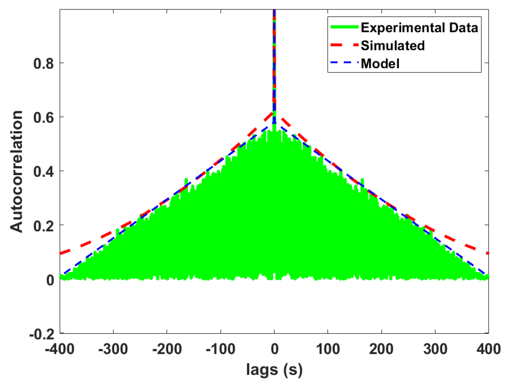
6. Phase Noise Generation Using the Modelled PDF and ACF
6.1. Phase Noise Generation Using the Modelled PDF
6.2. Phase Noise Generation Using the Modelled ACF
7. Conclusions
Author Contributions
Funding
Data Availability Statement
Conflicts of Interest
References
- Lewandowski, W.; Thomas, C. GPS time transfer. Proc. IEEE 1991, 79, 991–1000. [Google Scholar] [CrossRef]
- Imae, M.; Hosokawa, M.; Imamura, K.; Yukawa, H.; Shibuya, Y.; Kurihara, N.; Fisk, P.T.; Lawn, M.A.; Zhigang, L.; Huanxin, L.; et al. Two-way satellite time and frequency transfer networks in Pacific Rim region. IEEE Trans. Instrum. Meas. 2001, 50, 559–562. [Google Scholar] [CrossRef]
- Pánek, P.; Kodet, J.; Procházka, I. Accuracy of two-way time transfer via a single coaxial cable. Metrologia 2013, 50, 60. [Google Scholar] [CrossRef]
- Rost, M.; Piester, D.; Yang, W.; Feldmann, T.; Wübbena, T.; Bauch, A. Time transfer through optical fibres over a distance of 73 km with an uncertainty below 100 ps. Metrologia 2012, 49, 772. [Google Scholar] [CrossRef]
- Neelam; Olaniya, M.; Rathore, H.; Sharma, L.; Roy, A.; De, S.; Panja, S. Precise time synchronization and clock comparison through a White Rabbit network-based optical fiber link. Radio Sci. 2021, 56, 1–9. [Google Scholar] [CrossRef]
- White Rabbit Project Website. Available online: https://ohwr.org/project/white-rabbit/wikis/home (accessed on 9 March 2023).
- Kaur, N.; Tuckey, P.; Pottie, P.E. Time transfer over a White Rabbit network. In Proceedings of the 2016 European Frequency and Time Forum (EFTF), York, UK, 4–7 April 2016; pp. 1–4. [Google Scholar]
- Lipiński, M.; Włostowski, T.; Serrano, J.; Alvarez, P. White rabbit: A PTP application for robust sub-nanosecond synchronization. In Proceedings of the 2011 IEEE International Symposium on Precision Clock Synchronization for Measurement, Control and Communication, Munich, Germany, 12–16 September 2011; pp. 25–30. [Google Scholar]
- Hann, K.; Jobert, S.; Rodrigues, S. Synchronous ethernet to transport frequency and phase/time. IEEE Commun. Mag. 2012, 50, 152–160. [Google Scholar] [CrossRef]
- Dierikx, E.F.; Wallin, A.E.; Fordell, T.; Myyry, J.; Koponen, P.; Merimaa, M.; Pinkert, T.J.; Koelemeij, J.C.; Peek, H.Z.; Smets, R. White rabbit precision time protocol on long-distance fiber links. IEEE Trans. Ultrason. Ferroelectr. Freq. Control 2016, 63, 945–952. [Google Scholar] [CrossRef]
- Moreira, P.; Alvarez, P.; Serrano, J.; Darwezeh, I.; Wlostowski, T. Digital dual mixer time difference for sub-nanosecond time synchronization in Ethernet. In Proceedings of the 2010 IEEE International Frequency Control Symposium, Newport Beach, CA, USA, 1–4 June 2010; pp. 449–453. [Google Scholar]
- Moreira, P.; Serrano, J.; Wlostowski, T.; Loschmidt, P.; Gaderer, G. White rabbit: Sub-nanosecond timing distribution over ethernet. In Proceedings of the 2009 International Symposium on Precision Clock Synchronization for Measurement, Control and Communication, Brescia, Italy, 12–16 October 2009; pp. 1–5. [Google Scholar] [CrossRef]
- Marinov, M.B.; Ganev, B.; Djermanova, N.; Tashev, T.D. Analysis of Sensors Noise Performance Using Allan Deviation. In Proceedings of the 2019 IEEE XXVIII International Scientific Conference Electronics (ET), Sozopol, Bulgaria, 12–14 September 2019; pp. 1–4. [Google Scholar] [CrossRef]
- Jiang, L.A.; Wong, S.T.; Grein, M.E.; Ippen, E.P.; Haus, H.A. Measuring timing jitter with optical cross correlations. IEEE J. Quantum Electron. 2002, 38, 1047–1052. [Google Scholar] [CrossRef]
- Yadin, Y.; Shtaif, M.; Orenstein, M. Nonlinear phase noise in phase-modulated WDM fiber-optic communications. IEEE Photonics Technol. Lett. 2004, 16, 1307–1309. [Google Scholar] [CrossRef]
- Hadzi-Vukovic, J.; Jevtic, M.M.; Simic, D. Phase noise amplitude distribution as indicator of origin of random phase perturbation in a test oscillator. In Proceedings of the 2002 23rd International Conference on Microelectronics. Proceedings (Cat. No. 02TH8595), Nis, Yugoslavia, 12–15 May 2002; Volume 1, pp. 301–304. [Google Scholar]
- Rizzi, M.; Lipinski, M.; Ferrari, P.; Rinaldi, S.; Flammini, A. White rabbit clock synchronization: Ultimate limits on close-in phase noise and short-term stability due to FPGA implementation. IEEE Trans. Ultrason. Ferroelectr. Freq. Control 2018, 65, 1726–1737. [Google Scholar] [CrossRef] [PubMed]
- Rizzi, M.; Ferrari, P.; Flammini, A.; Rinaldi, S.; Sisinni, E. Characterization of 1 Gbps fiber optics transceiver for high accuracy synchronization over Ethernet. In Proceedings of the 2018 IEEE International Instrumentation and Measurement Technology Conference (I2MTC), Houston, TX, USA, 14–17 May 2018; pp. 1–6. [Google Scholar]
- Li, P.; Gong, H.; Peng, J.; Zhu, X. Time synchronization of white rabbit network based on kalman filter. In Proceedings of the 2019 3rd International Conference on Electronic Information Technology and Computer Engineering (EITCE), Xiamen, China, 18–20 October 2019; pp. 572–576. [Google Scholar]
- Keysight, 53,200 Series Datasheet and User’s Manual. Available online: https://www.keysight.com/in/en/assets/9018-03351/user-manuals/9018-03351.pdf?success=true (accessed on 9 March 2023).
- TDC Datasheet and User Guide. Available online: https://www.ti.com/lit/ds/symlink/tdc7200.pdf?ts=1652248946865&ref (accessed on 19 March 2023).
- Ad9912 DDS Datasheet and User Guide. Available online: https://www.analog.com/media/en/technical-documentation/user-guides/EVAL-AD9912A_PCBZ_UG-475.pdf (accessed on 9 March 2023).
- Savory, J.; Sherman, J.; Romisch, S. White Rabbit-Based Time Distribution at NIST. In Proceedings of the 2018 IEEE International Frequency Control Symposium (IFCS), Olympic Valley, CA, USA, 21–24 May 2018; pp. 1–5. [Google Scholar] [CrossRef]
- Neelam; Rathore, H.; Sharma, L.; Roy, A.; Olaniya, M.; De, S.; Panja, S. Studies on Temperature Sensitivity of a White Rabbit Network-Based Time Transfer Link. MAPAN 2021, 36, 253–258. [Google Scholar] [CrossRef]
- Generating Samples from Probability Distribution. Available online: https://web.mit.edu/urban_or_book/www/book/chapter7/7.1.3.html (accessed on 9 May 2023).
- Direct formulation to Cholesky decomposition of a general nonsingular correlation matrix. Stat. Probab. Lett. 2015, 103, 142–147. [CrossRef] [PubMed]


| Data Sets | Optical Fibre Links | Mixing Component (K) | GMM Mean () | GMM Sigma () | Component Proportion () |
|---|---|---|---|---|---|
| Data set 1: Phase offset between WRLEN1 and WRLEN2 at T = 1 ms | between WRLEN1 and WRLEN2 with a 10 km fibre | 5 | −0.0422385; −0.0366300; 0.0026105; 0.0396109; 0.0878236 | 0.0030000; 0.0008299; 0.0001102; 0.0001412; 0.0003211 | 0.010; 0.430; 0.280; 0.220; 0.060 |
| Data set 2: Phase offset between WRLEN2 and WRLEN3 at T = 1 ms | between WRLEN2 and WRLEN3 with a 10 km fibre | 5 | −0.0906074; −0.0398586; 0.0076509; 0.0454425; 0.0929520 | 0.0001955; 0.0001685; 0.0001506; 0.0000892; 0.0004190 | 0.030; 0.320; 0.480; 0.130; 0.040 |
| Data set 3: Phase offset between WRLEN1 and WRLEN3 at T = 1 ms | between WRLEN1 and WRLEN3 through WRLEN2 with 20 km fibres | 8 | −0.1293010; −0.0835311; −0.0421908; −0.0008504; 0.0493486; 0.0921653; 0.1305530; 0.1293010 | 0.0003055; 0.0002317; 0.0001715; 0.0002135; 0.0002798; 0.0003369; 0.0003994; 0.0004055 | 0.020; 0.170; 0.180; 0.220; 0.260; 0.110; 0.030; 0.010 |
| Data set 4: Phase offset between WRLEN2 and WRLEN3 at T = 1 s | between WRLEN2 and WRLEN3 with a 10 km fibre | 6 | −0.0669749; −0.0739749; −0.0415965; −0.0092181; 0.0315547; 0.0711283 | 0.0018900; 0.0009905; 0.0008999; 0.0001819; 0.0001835; 0.0002911 | 0.010; 0.020; 0.340; 0.320; 0.240; 0.070 |
| Data set 5: Phase offset between WRLEN1 and WRLEN2 at T = 1 s | between WRLEN1 and WRLEN2 with a 10 km fibre | 7 | −0.0986648; −0.0569917; −0.0266839; −0.0020589; 0.0301430; 0.0727634; 0.1172780 | 0.0003855; 0.0002292; 0.0000625; 0.0000870; 0.0001800; 0.0003519; 0.0003794 | 0.040; 0.210; 0.150; 0.190; 0.220; 0.160; 0.03 |
| Data Sets | Optical Fibre Links | Mixing Component (K) | GMM Mean () | GMM Sigma () | Component Proportion () |
|---|---|---|---|---|---|
| Data set 6: Phase offset between WRLEN1 and WRLEN2 at T = 1 ms | between WRLEN1 and WRLEN2 with 50 km fibre | 8 | −0.0933650; −0.0588505; −0.0358408; −0.0128311; 0.0170825; 0.0343380; 0.0596495; 0.0941641 | 0.0003211; 0.0002950; 0.0001987; 0.0001260; 0.0001282; 0.0001312; 0.0001982; 0.0003940; | 0.048; 0.125; 0.115; 0.235; 0.197; 0.105; 0.120; 0.055; |
| Data set 7: Phase offset between WRLEN2 and WRLEN3 at T = 1 ms | between WRLEN2 and WRLEN3 with a 50 km fibre | 8 | −0.0981730; −0.0614800; −0.0362600; −0.0133300; 0.0118910; 0.0382600; 0.0588980; 0.0955860; | 0.0003900; 0.0002650; 0.0001327; 0.0000897; 0.0000999; 0.0003319; 0.0003680; 0.0003940; | 0.060; 0.120; 0.140; 0.170; 0.200; 0.220; 0.050; 0.040; |
| Data set 8: Phase offset between WRLEN1 and WRLEN3 at T = 1 ms | between WRLEN1 and WRLEN3 through WRLEN2 with a 100 km fibre | 6 | −0.1126410, −0.0764358; −0.0323600; 0.0101400; 0.0542160; 0.0951431; | 0.0030000, 0.0004750; 0.0001616; 0.0001895; 0.0002499; 0.0001500; | 0.040, 0.160; 0.240; 0.300; 0.200; 0.060; |
| Data Set | Test Setup | Optical Fibre Links | a | b |
|---|---|---|---|---|
| Data set 1: Phase offset between WRLEN1 and WRLEN2 at T = 1 ms | A with HROG-10 | between WRLEN1 and WRLEN2 with 10 km fibre | 1200 | 0.36 |
| Data set 2: Phase offset between WRLEN2 and WRLEN3 at T = 1 ms | A with HROG-10 | between WRLEN2 and WRLEN3 with 10 km fibre | 2300 | 0.20 |
| Data set 3: Phase offset between WRLEN1 and WRLEN2 at T = 1 ms | A with HROG-10 | between WRLEN1 and WRLEN3 with 20 km fibre | 580 | 0.70 |
| Data set 4: Phase offset between WRLEN2 and WRLEN3 at T = 1 s | A with HROG-10 | between WRLEN2 and WRLEN3 with 10 km fibre | 2200 | 0.20 |
| Data set 5: Phase offset between WRLEN1 and WRLEN2 at T = 1 s | A with HROG-10 | between WRLEN1 and WRLEN2 with 10 km fibre | 700 | 0.58 |
| Data set 6: Phase offset between WRLEN1 and WRLEN2 at T = 1 ms | B with the testbed | between WRLEN1 and WRLEN2 with 50 km fibre | 930 | 0.46 |
| Data set 7: Phase offset between WRLEN2 and WRLEN3 at T = 1 ms | B with the testbed | between WRLEN2 and WRLEN3 with 50 km fibre | 930 | 0.46 |
| Data set 8: Phase offset between WRLEN1 and WRLEN3 at T = 1 ms | B with the testbed | between WRLEN1 and WRLEN3 through WRLEN2 with 100 km fibre | 930 | 0.46 |
Disclaimer/Publisher’s Note: The statements, opinions and data contained in all publications are solely those of the individual author(s) and contributor(s) and not of MDPI and/or the editor(s). MDPI and/or the editor(s) disclaim responsibility for any injury to people or property resulting from any ideas, methods, instructions or products referred to in the content. |
© 2024 by the authors. Licensee MDPI, Basel, Switzerland. This article is an open access article distributed under the terms and conditions of the Creative Commons Attribution (CC BY) license (https://creativecommons.org/licenses/by/4.0/).
Share and Cite
Neelam; Kandeepan, S.; Panja, S. Phase Noise Analysis of Time Transfer over White Rabbit-Network Based Optical Fibre Links. Sensors 2024, 24, 381. https://doi.org/10.3390/s24020381
Neelam, Kandeepan S, Panja S. Phase Noise Analysis of Time Transfer over White Rabbit-Network Based Optical Fibre Links. Sensors. 2024; 24(2):381. https://doi.org/10.3390/s24020381
Chicago/Turabian StyleNeelam, Sithamparanathan Kandeepan, and Subhasis Panja. 2024. "Phase Noise Analysis of Time Transfer over White Rabbit-Network Based Optical Fibre Links" Sensors 24, no. 2: 381. https://doi.org/10.3390/s24020381
APA StyleNeelam, Kandeepan, S., & Panja, S. (2024). Phase Noise Analysis of Time Transfer over White Rabbit-Network Based Optical Fibre Links. Sensors, 24(2), 381. https://doi.org/10.3390/s24020381