
A Proposed Algorithm Based on Variance to Effectively Estimate Crack Source Localization in Solids


Abstract
1. Introduction
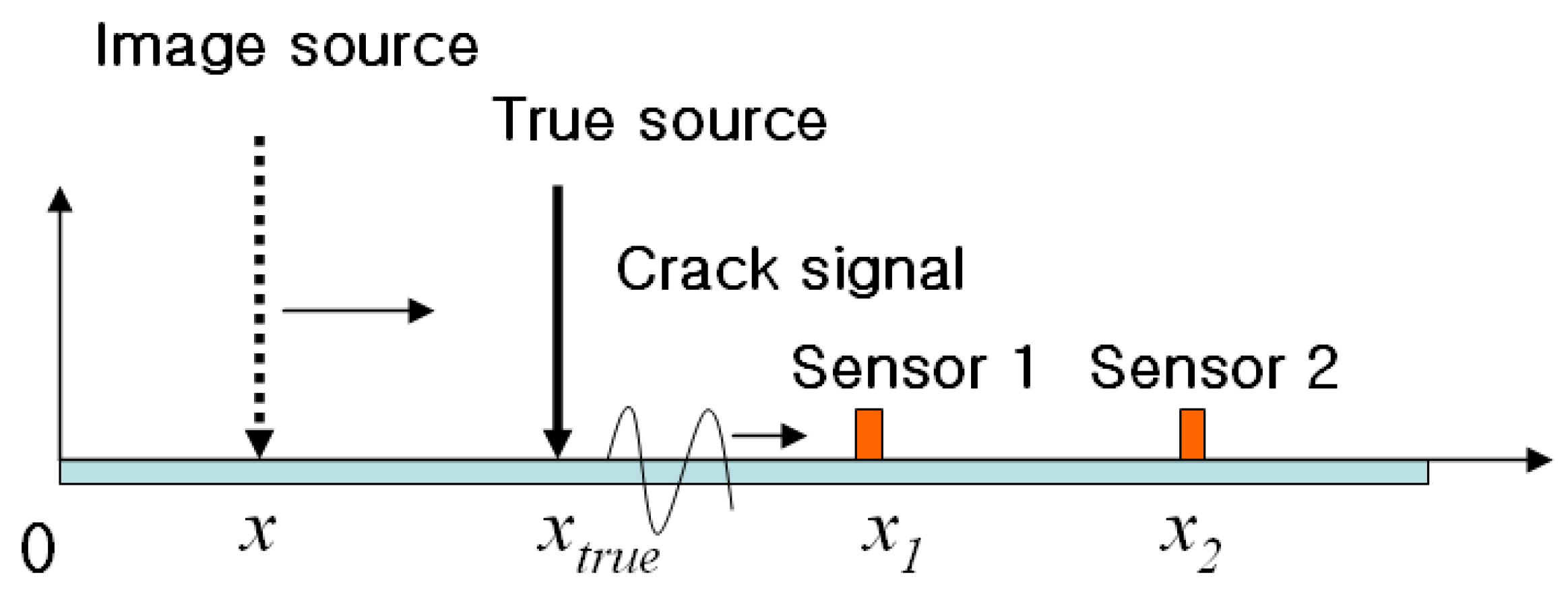
2. Basic Idea
3. Background Theory for Finding TOAD
4. Source Localization Algorithm
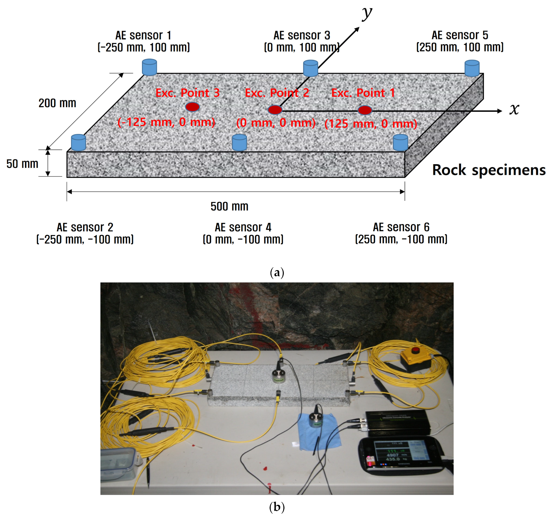
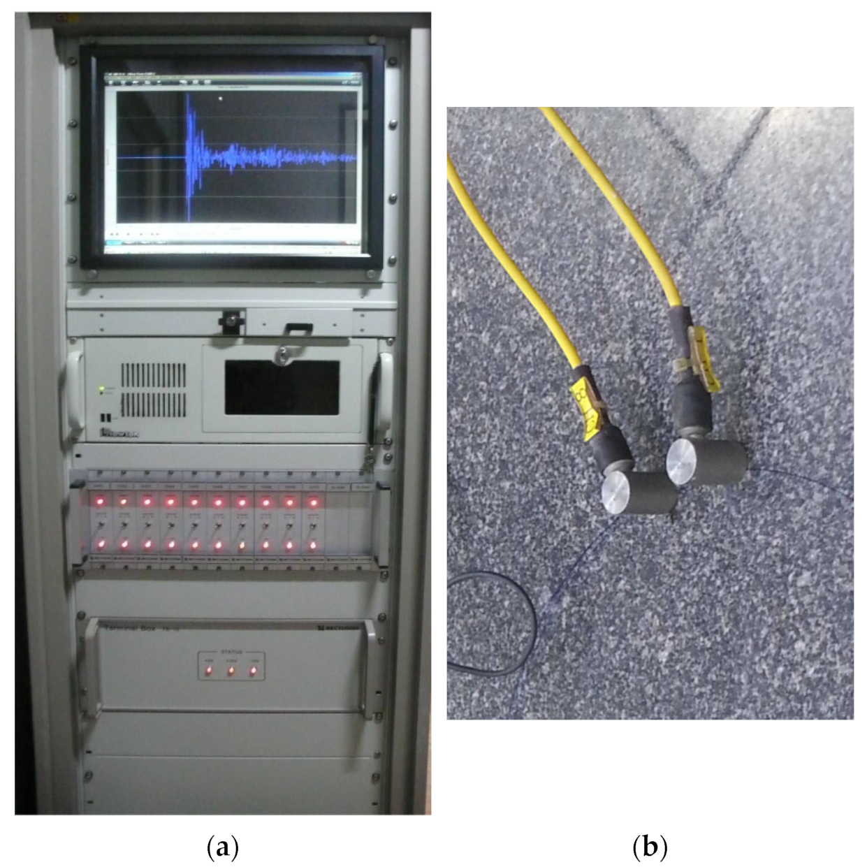
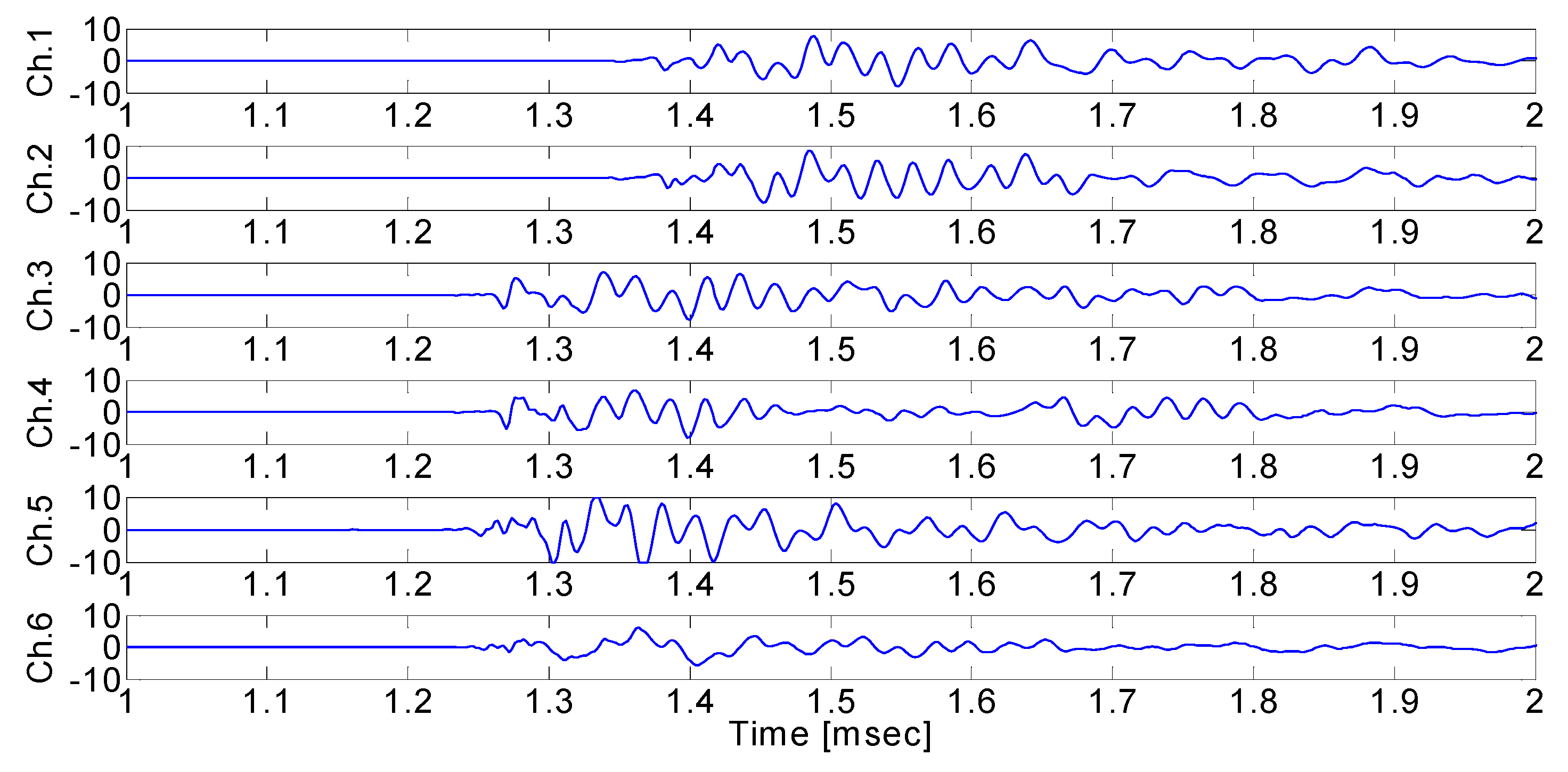
5. Validation Using an Experiment
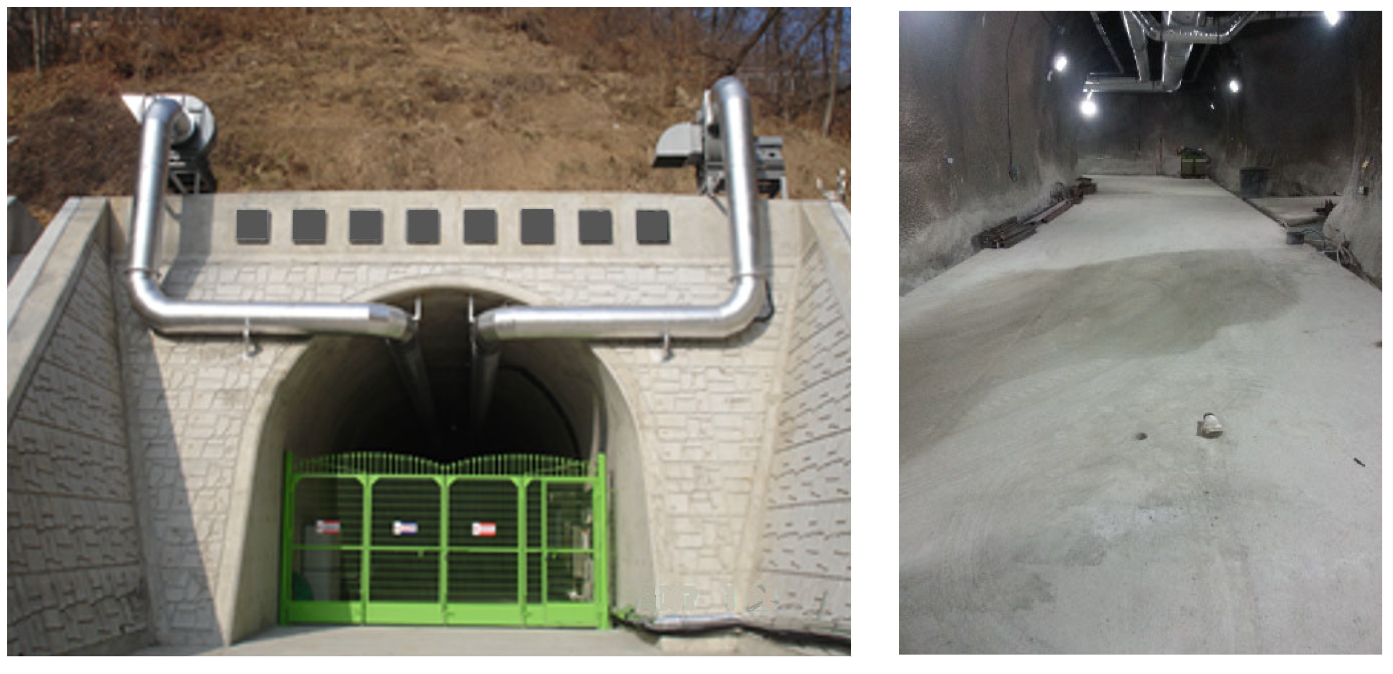
6. Verification Test at In Situ Test
7. Conclusions
- The effective detection of extremely early fatigue damage in structures, including aircraft.
- The safety assessment of civil structures, including steel and concrete bridges and dams.
- The diagnosis of in-process processes (e.g., welding monitoring).
- As a means of testing, evaluating, and identifying the mechanical properties and fracture mechanisms of materials.
- The detection and determination of the location of defects in pressure vessels, including nuclear reactors, etc.
Author Contributions
Funding
Institutional Review Board Statement
Informed Consent Statement
Data Availability Statement
Conflicts of Interest
References
- Tsang, C.F.; Bernier, F.; Davies, C. Geohydromechanical processes in the excavation damaged zone in crystalline rock, rock salt, and indurated and plastic calys-in the context of radioactive waste disposal. Int. J. Rock Mech. Min. Sci. 2005, 42, 109–125. [Google Scholar] [CrossRef]
- IAEA-TECDOC-1208; Monitoring of Geological Repositories for High Level Radioactive Waste. IAEA: Vienna, Austria, 2001.
- EU. Thematic Network on the Role of Monitoring in a Phased Approach to Geological Disposal of Radioactive Waste; Final Report to the European Commission Contract FIKW-CT-2001-20130; U.S. Department of Energy: Washington, DC, USA, 2004; pp. 1–16.
- Hardy, H.R. Geotechnical field applications of AE/MS techniques at the Pennsylvania State University: A historical review. NDTE Int. 1994, 27, 191–200. [Google Scholar] [CrossRef]
- Arvin, E.; Choi, J.; Trevor, D.; Salvatore, S. Acoustic emission monitoring of containment structures during post-tensioning. Eng. Struct. 2020, 209, 109930. [Google Scholar]
- Li, S.; Chang, S.; Li, P.; Zhang, X.; Jiang, N. Optimization of concrete surface sensor arrangement for acoustic emission monitoring of prestressed steel strand damage in T-beams. Appl. Acoust. 2024, 223, 110082. [Google Scholar] [CrossRef]
- Guo, R.; Zhang, X.; Lin, X.; Huang, S. Active and passive monitoring of corrosion state of reinforced concrete based on embedded cement-based acoustic emission sensor. J. Build. Eng. 2024, 89, 109276. [Google Scholar] [CrossRef]
- Chen, J.; Tong, J.; Rui, Y.; Cui, Y.; Pu, Y.; Du, J.; Apel, D.B. Step-path failure mechanism and stability analysis of water-bearing rock slopes based on particle flow simulation. Theor. Appl. Fract. Mech. 2024, 131, 104370. [Google Scholar] [CrossRef]
- Tsunoda, T.; Kato, T.; Hirata, K.; Sekido, Y.; Segawa, M.; Ymamtoku, S.; Morioka, T.; Sano, K.; Tsuneoka, O. Studies on the loose part evaluation technique. Prog. Nucl. Energy 1985, 15, 569–576. [Google Scholar] [CrossRef]
- Olma, B.J. Source location and mass estimation in loose parts monitoring of LWR’s. Prog. Nucl. Energy 1985, 15, 583–593. [Google Scholar] [CrossRef]
- Ciampa, F.; Meo, M. A new algorithm for acoustic emission localization and flexural group velocity determination in anisotropic structures. Compos. Part A. Appl. Sci. Manuf. 2010, 41, 1777–1786. [Google Scholar] [CrossRef]
- Jeong, H.; Jang, Y.S. Fracture source location in thin plates using the wavelet transform of dispersive waves. IEEE Trans. Ultras. Ferroelectr. Freq. Control. 2000, 47, 612–619. [Google Scholar] [CrossRef] [PubMed]
- Yaghin, M.A.L.; Koohdaragh, M. Examining the function of wavelet packet transform(WPT) and continues wavelet transform(CWT) in recognizing the crack specification. KSCE J. Civ. Eng. 2011, 15, 497–506. [Google Scholar] [CrossRef]
- Park, J.H.; Kim, Y.H. Impact source localization on an elastic plate in a noisy environment. Meas. Sci. Technol. 2006, 17, 2757–2766. [Google Scholar] [CrossRef]
- Li, Y.; Zheng, X. Wigner-Ville distribution and its application in seismic attenuation estimation. J. Appl. Geophys. 2007, 30, 245–254. [Google Scholar] [CrossRef]
- Choi, Y.C.; Kim, J.S.; Park, T.J. Estimating arrival time of crack wave by using moving window. In Proceedings of the Korean Radioactive Waste Society Spring Conference, Deajeon, Republic of Korea, 24–26 May 2017. [Google Scholar]
- Choi, Y.C.; Park, T.J. A method for detecting crack wave arrival time and crack localization in an tunnel by using moving window technique. In Proceedings of the Transaction of the Korean Nuclear Society Spring Meeting, Jeju, Republic of Korea, 12–13 May 2016. [Google Scholar]


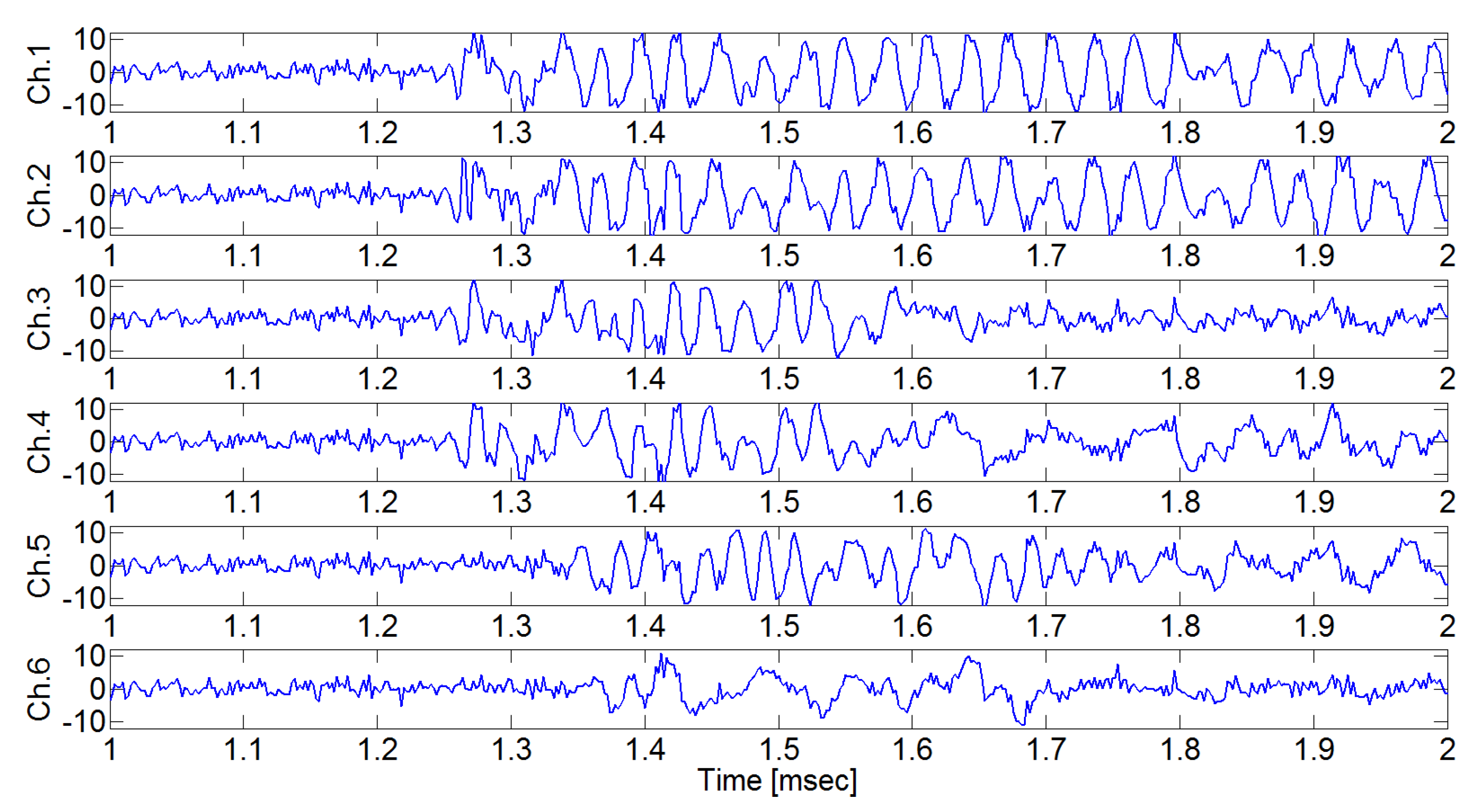
| Exc. Point 1 (−125 mm, 0 mm) | Exc. Point 2 (0 mm, 0 mm) | Exc. Point 3 (125 mm, 0 mm) | |
|---|---|---|---|
| Arrival Time | Arrival Time | Arrival Time | |
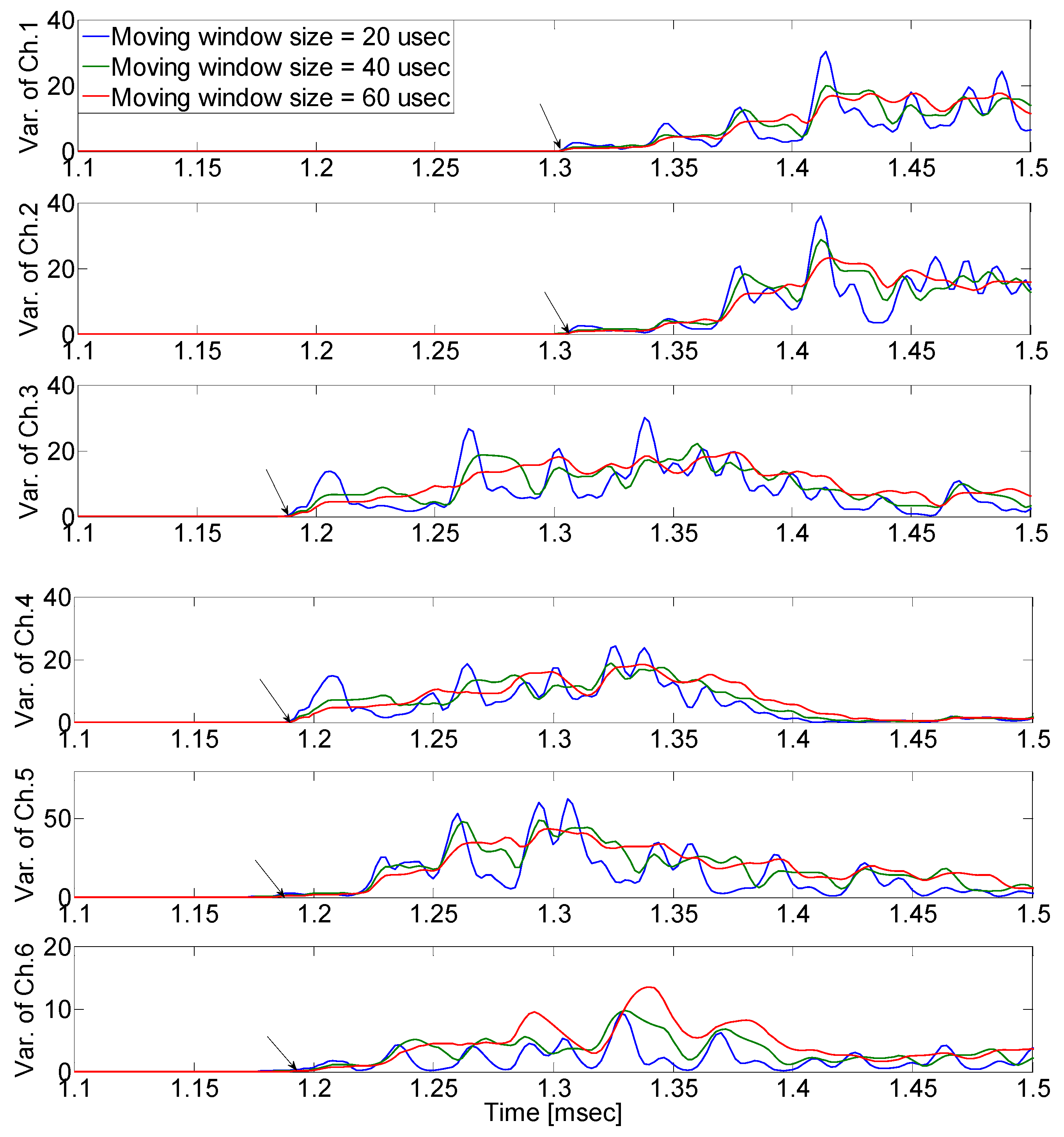
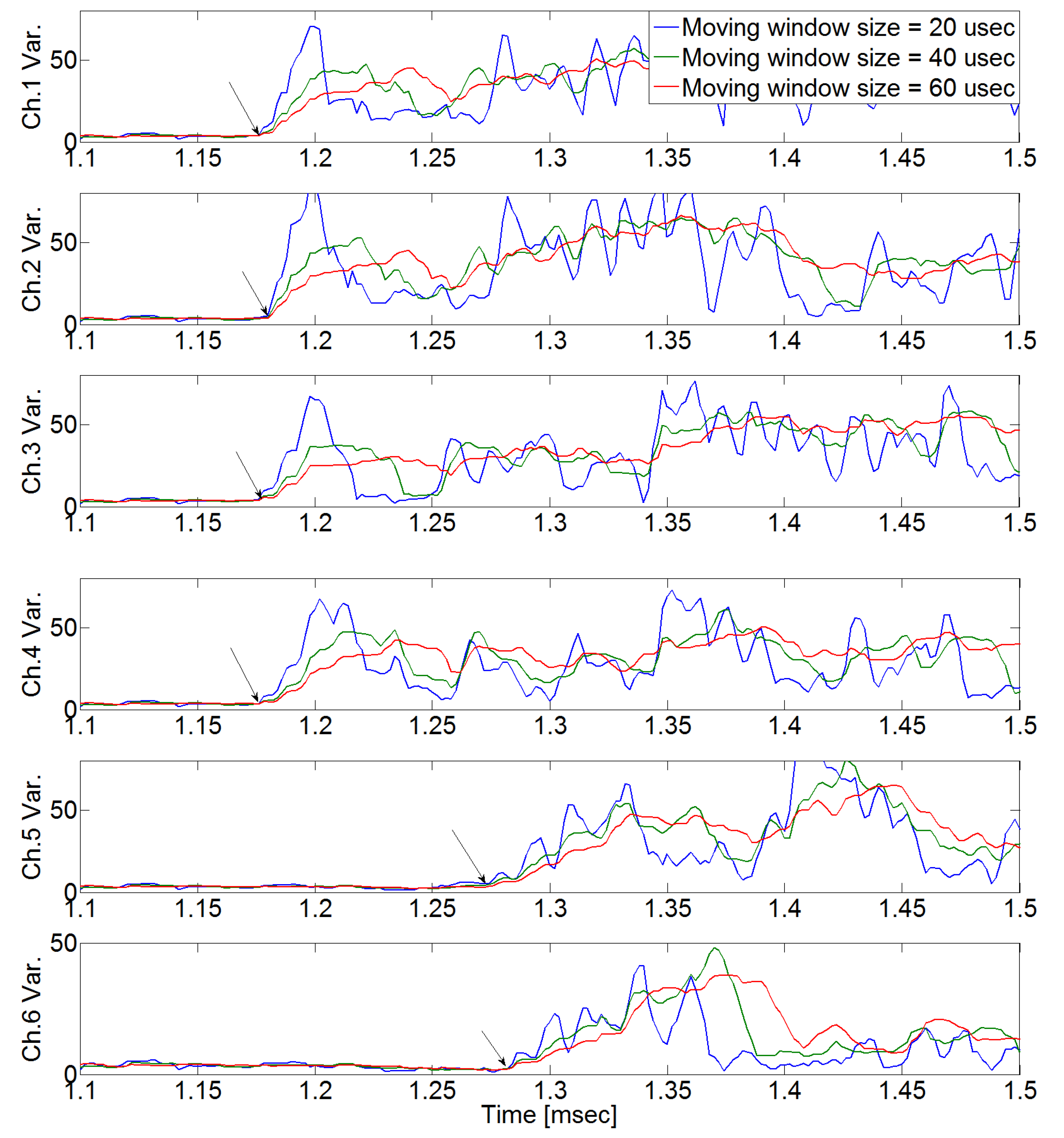
| Ch. 1 | 1.302 msec | 1.232 msec | 1.174 msec |
| Ch. 2 | 1.304 msec | 1.236 msec | 1.175 msec |
| Ch. 3 | 1.189 msec | 1.170 msec | 1.174 msec |
| Ch. 4 | 1.190 msec | 1.170 msec | 1.176 msec |
| Ch. 5 | 1.188 msec | 1.234 msec | 1.252 msec |
| Ch. 6 | 1.191 msec | 1.235 msec | 1.254 msec |
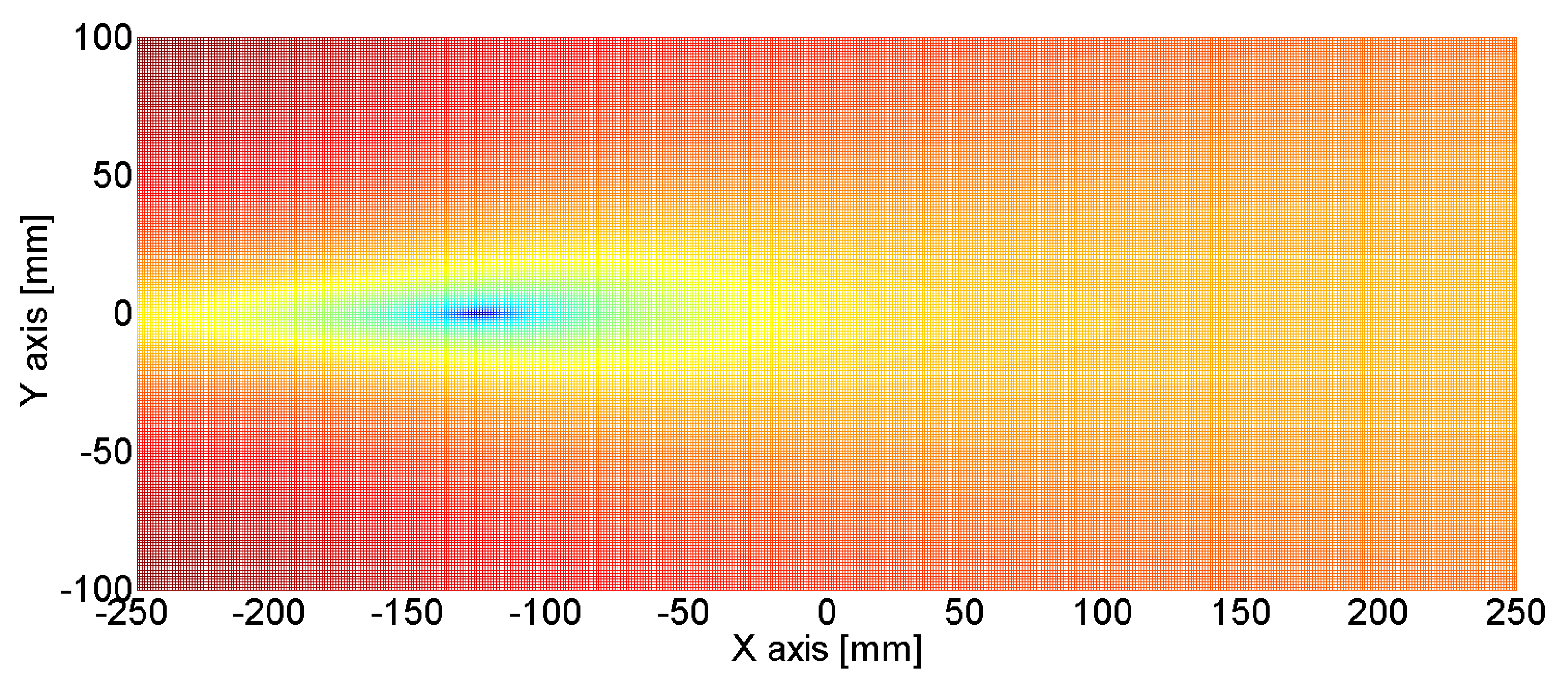
| Source Locations (x, y) | |||
|---|---|---|---|
| True source locations | Excitation point 3 (−125 mm, 0 mm) | Excitation point 2 (0 mm, 0 mm) | Excitation point 1 (125 mm, 0 mm) |
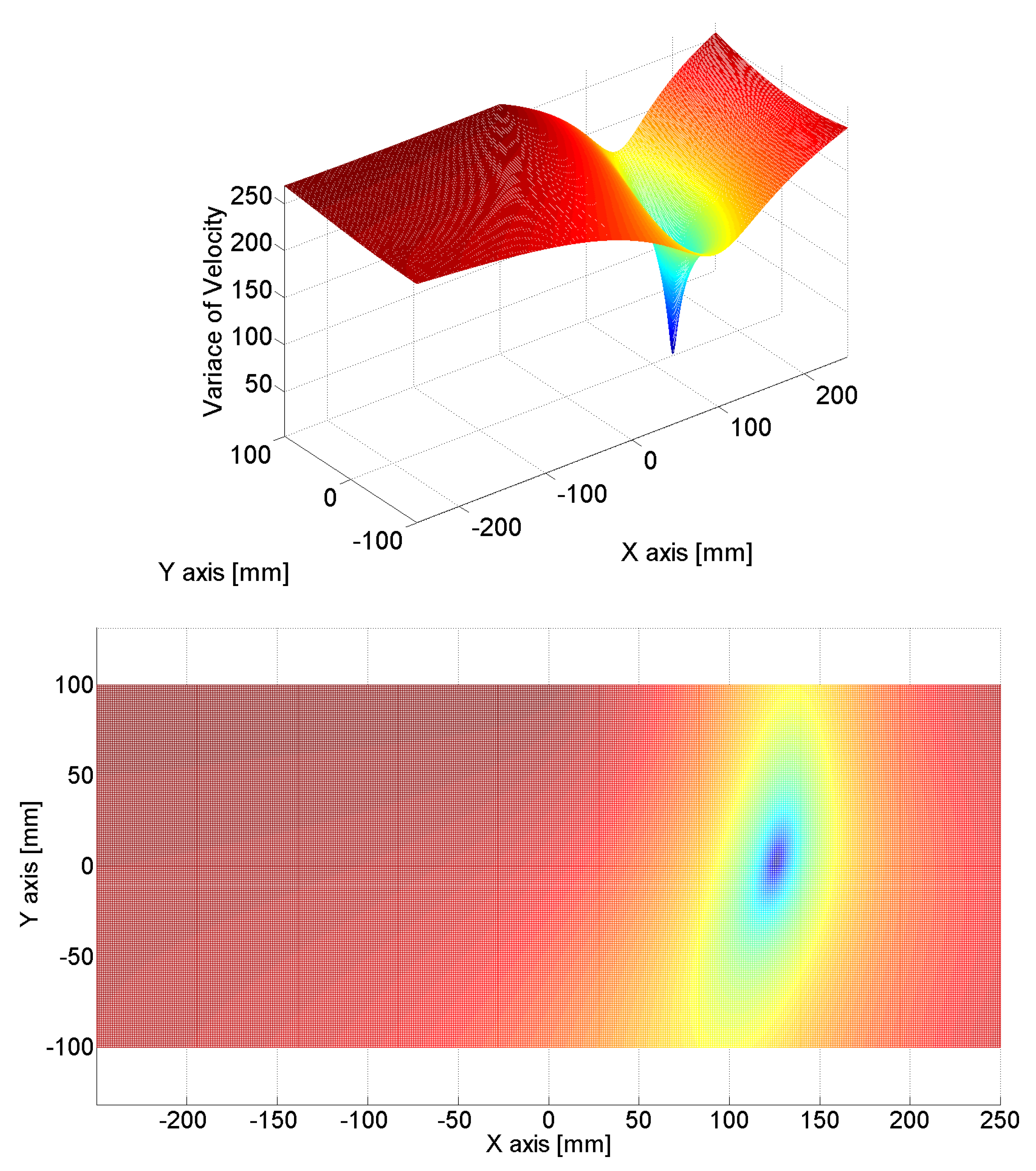
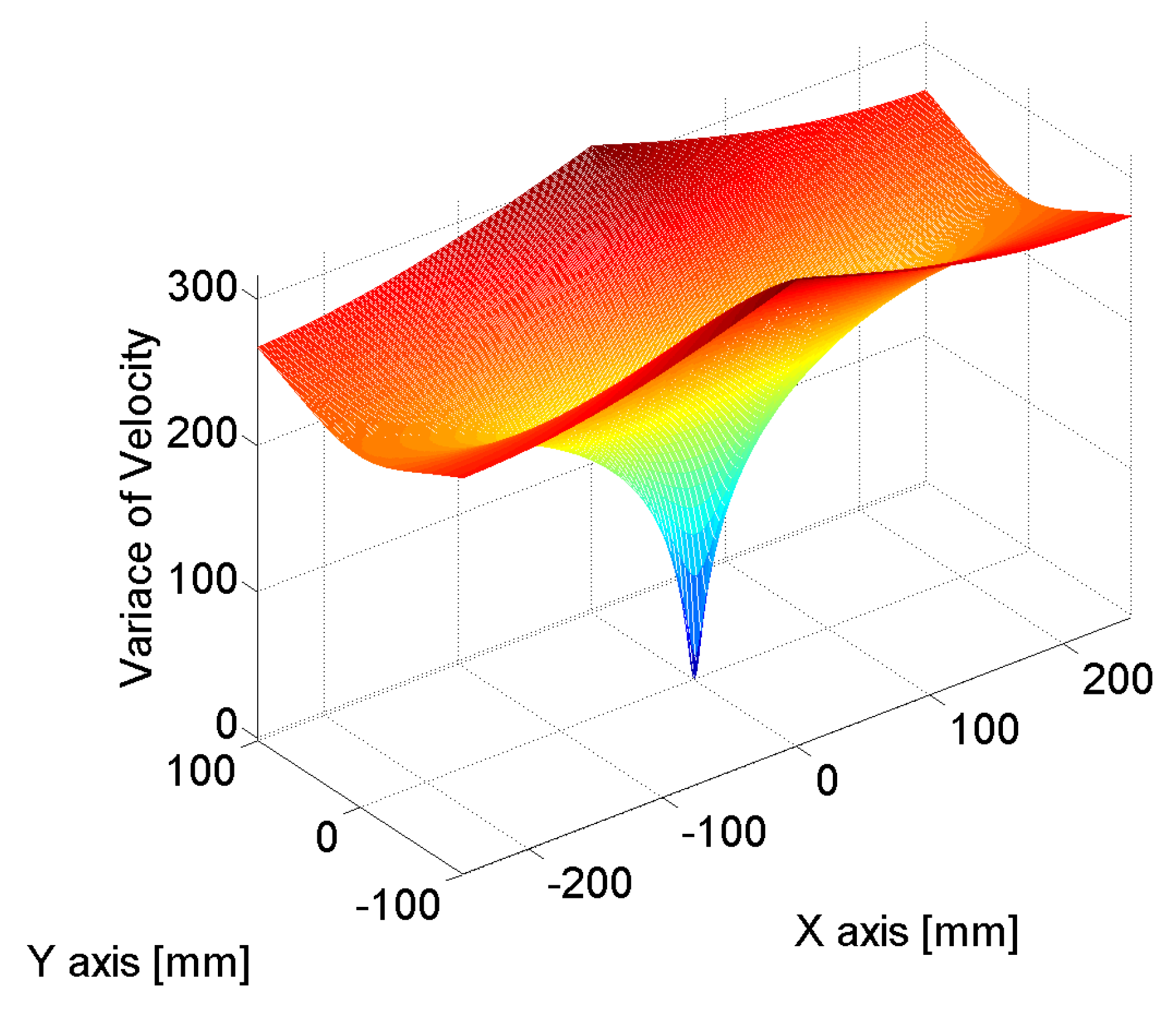
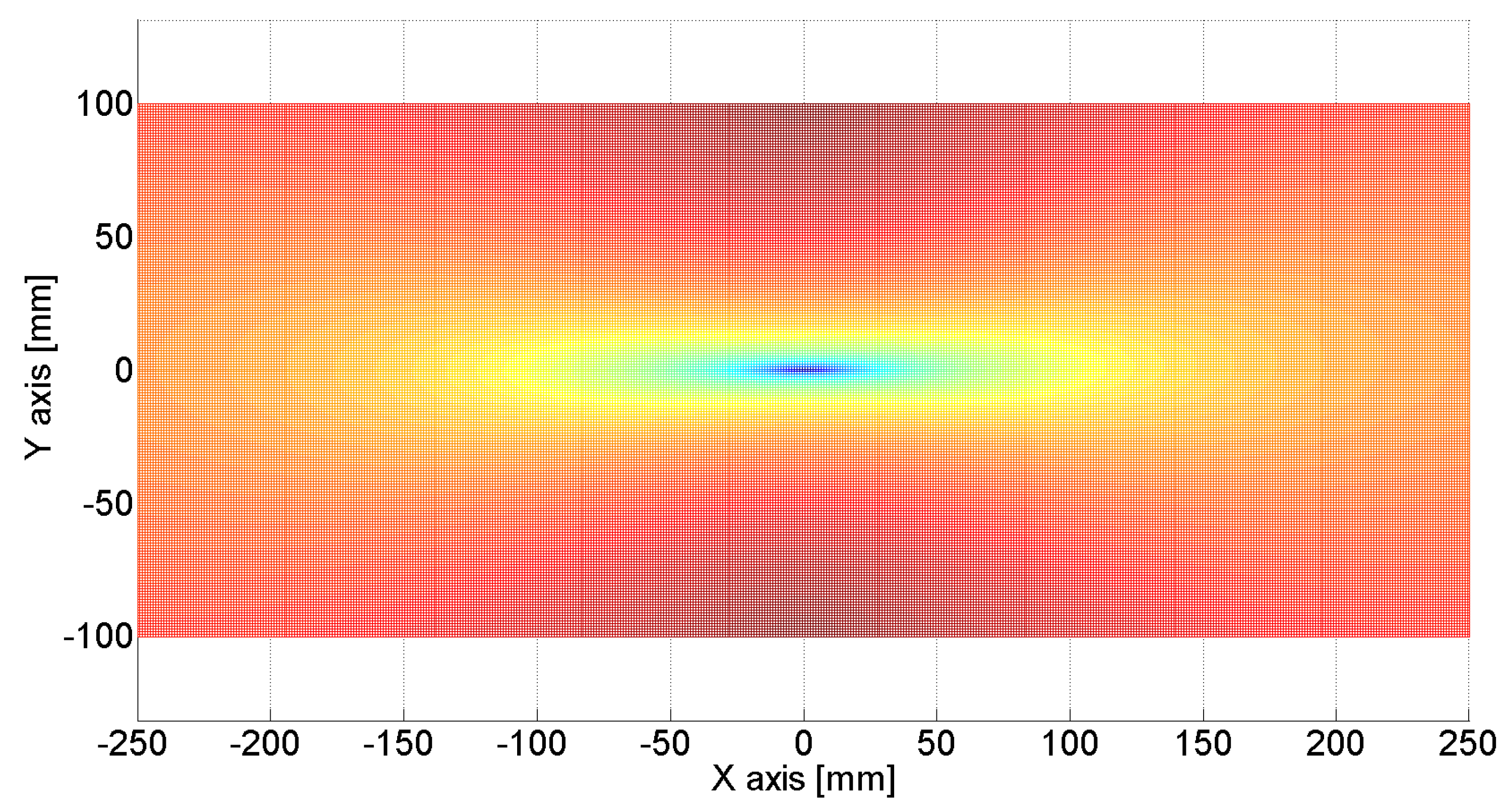
| Estimated source locations | (−125.8 mm, 2.7 mm) | (−0.5 mm, 0.5 mm) | (−124.7 mm, 1.5 mm) |
| Distance error btw true and estimated location | 2.8 mm | 0.7 mm | 1.5 mm |
| Sensor | Estimated Arrival Time at Excitation Point 1 | Estimated Arrival Time at Excitation Point 2 | ||
|---|---|---|---|---|
| Conventional Method | Proposed Method | Conventional Method | Proposed Method | |
| Sensor 1 | 0.672 msec | 0.420 msec | 0.668 msec | 0.168 msec |
| Sensor 2 | 0.592 msec | 0.268 msec | 0.542 msec | 0.256 msec |
| Sensor 3 | 0.542 msec | 0.208 msec | 0.628 msec | 0.238 msec |
| Sensor 4 | 0.472 msec | 0.232 msec | 0.640 msec | 0.308 msec |
| Sensor 5 | 0.788 msec | 0.421 msec | 0.670 msec | 0.330 msec |
| Sensor 6 | 0.672 msec | 0.292 msec | 0.494 msec | 0.382 msec |
| Sensor 7 | 0.484 msec | 0.159 msec | 0.518 msec | 0.342 msec |
| Sensor 8 | 0.448 msec | 0.160 msec | 0.500 msec | 0.396 msec |
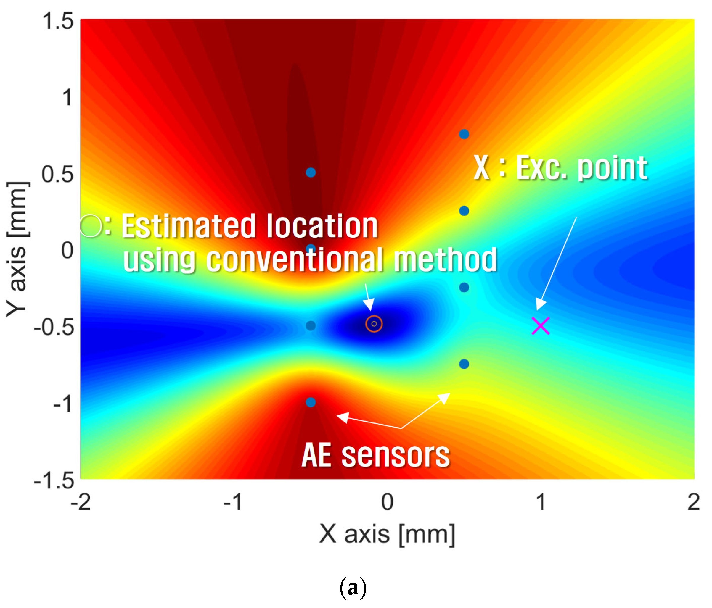
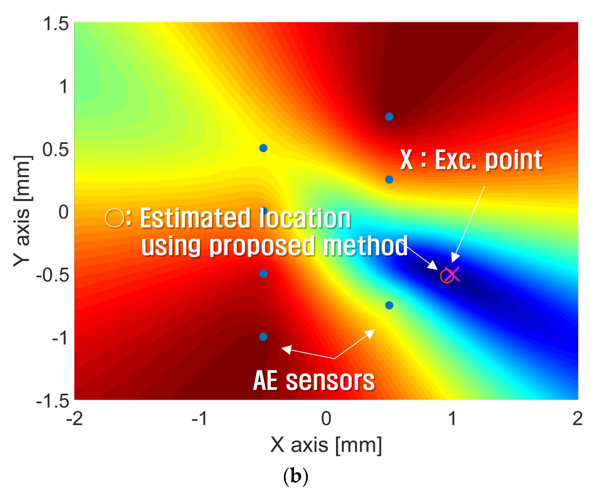
| Exc. Point | True Location | Conventional Method | Proposed Method | ||
|---|---|---|---|---|---|
| Estimated Location | Error | Estimated Location | Error | ||
| 1 | (−0.25 m, 0.25 m) | (0 m, 0.399 m) | 0.291 m | (−0.267 m, 0.248 m) | 0.171 m |
| 2 | (1.0 m, −0.5 m) | (−0.09 m, −0.49 m) | 1.09 m | (0.98 m, −0.52 m) | 0.028 m |
Disclaimer/Publisher’s Note: The statements, opinions and data contained in all publications are solely those of the individual author(s) and contributor(s) and not of MDPI and/or the editor(s). MDPI and/or the editor(s) disclaim responsibility for any injury to people or property resulting from any ideas, methods, instructions or products referred to in the content. |
© 2024 by the authors. Licensee MDPI, Basel, Switzerland. This article is an open access article distributed under the terms and conditions of the Creative Commons Attribution (CC BY) license (https://creativecommons.org/licenses/by/4.0/).
Share and Cite
Choi, Y.-C.; Chung, B.; Jung, D. A Proposed Algorithm Based on Variance to Effectively Estimate Crack Source Localization in Solids. Sensors 2024, 24, 6092. https://doi.org/10.3390/s24186092
Choi Y-C, Chung B, Jung D. A Proposed Algorithm Based on Variance to Effectively Estimate Crack Source Localization in Solids. Sensors. 2024; 24(18):6092. https://doi.org/10.3390/s24186092
Chicago/Turabian StyleChoi, Young-Chul, Byunyoung Chung, and Doyun Jung. 2024. "A Proposed Algorithm Based on Variance to Effectively Estimate Crack Source Localization in Solids" Sensors 24, no. 18: 6092. https://doi.org/10.3390/s24186092
APA StyleChoi, Y.-C., Chung, B., & Jung, D. (2024). A Proposed Algorithm Based on Variance to Effectively Estimate Crack Source Localization in Solids. Sensors, 24(18), 6092. https://doi.org/10.3390/s24186092