


Confidence Interval Estimation for Cutting Tool Wear Prediction in Turning Using Bootstrap-Based Artificial Neural Networks


Abstract
1. Introduction
2. Methodology
- A database containing mainly cutting forces from turning tests is used.
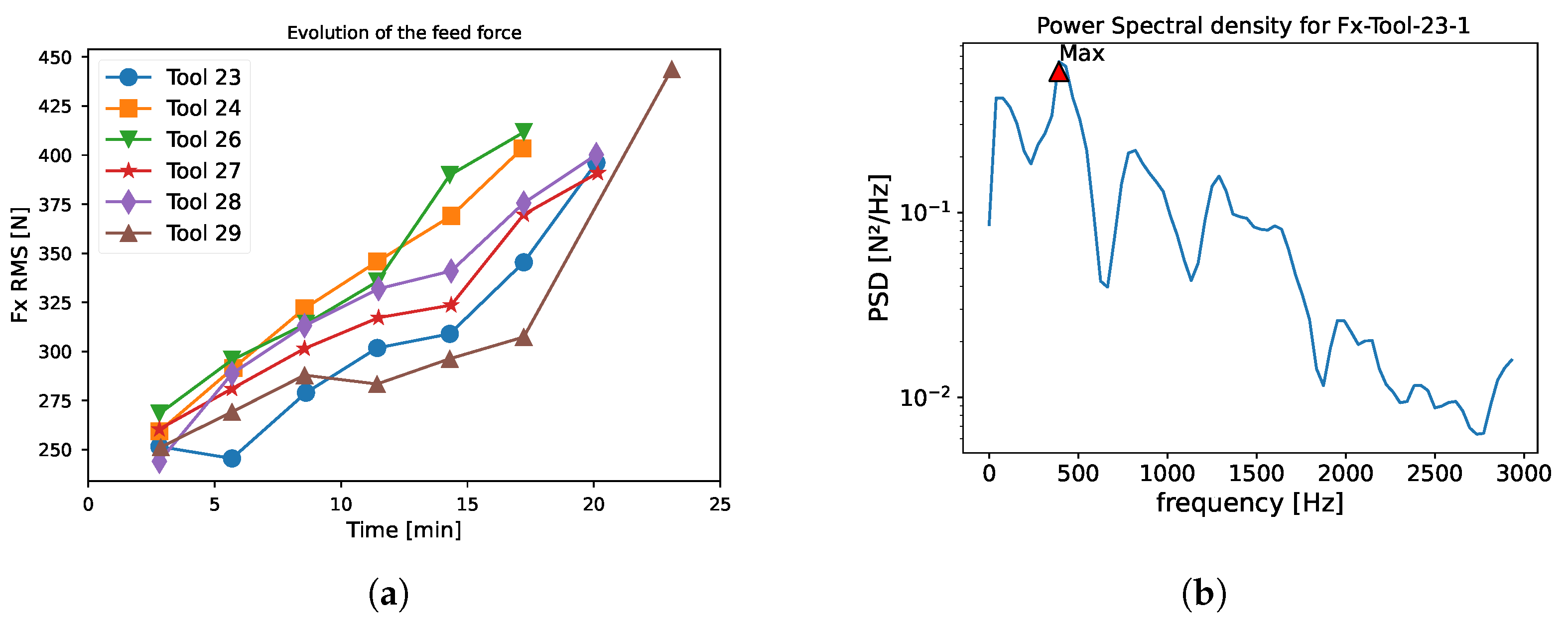
- The database, containing the raw force data, needs to be processed. As commonly realized in AI, these temporal force signals are preprocessed to obtain indicators, either statistical (root mean squared, skewness, etc.) or frequency (power spectral density).
- These indicators are not all correlated with the wear of the cutting tool; a selection of the most correlated indicator is therefore necessary to avoid using irrelevant information to train the network. Therefore, to find the best input for the networks, a correlation analysis is performed to establish the correlation between the tool wear and the computed indicator. An indicator with a high correlation to the tool wear is then used as an input for the the neural network. These inputs are standardized.
- The network is optimized to find the best architecture and combination of hyperparameters in order to achieve the best results. Once the best architecture is identified, the bootstrap method is applied to estimate the confidence interval around the prediction.
- The results are tested on previously unseen cutting speed variations in order to assess the capability of the network to generalize the results.
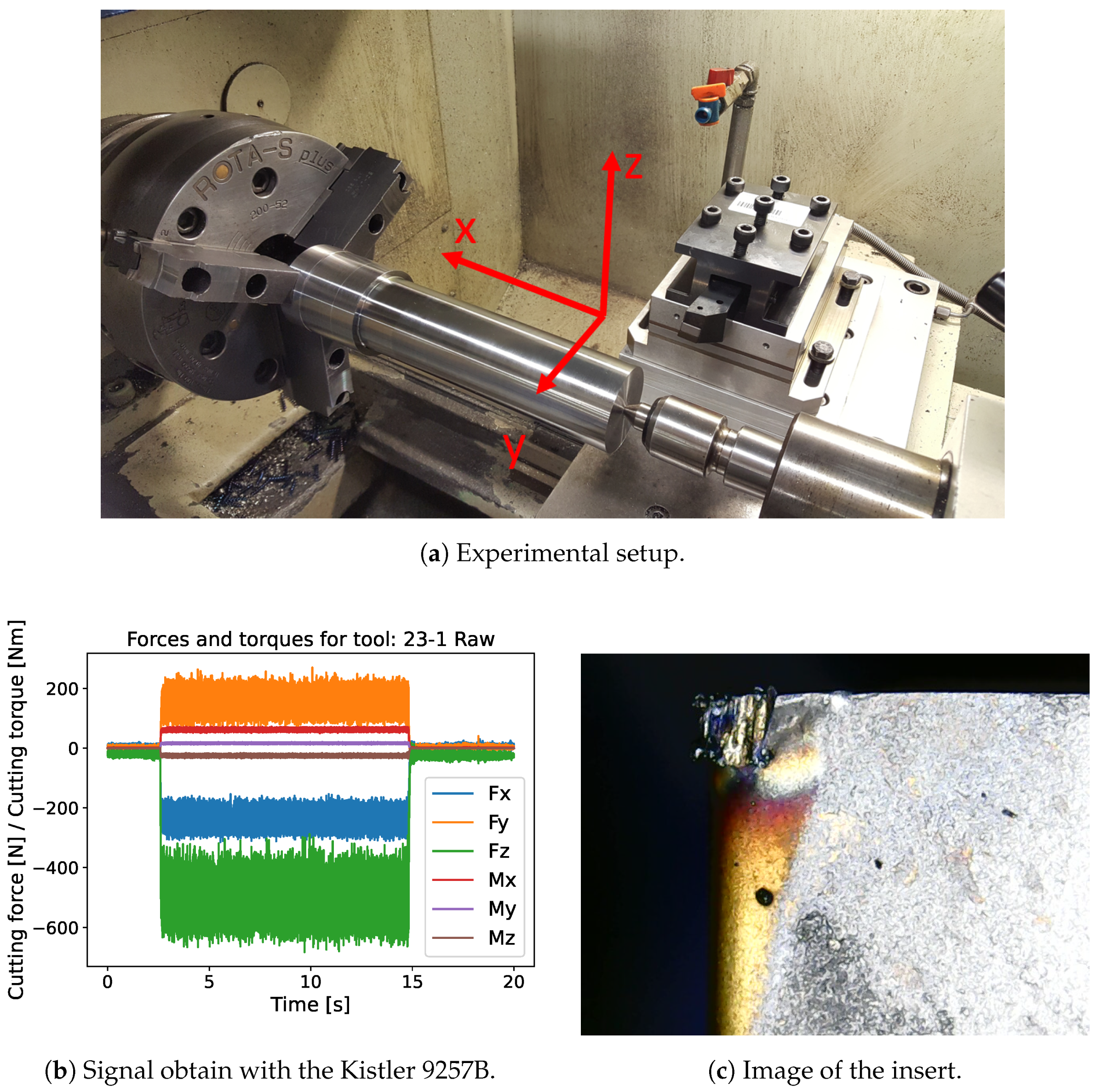
2.1. Experimental Setup
2.2. Features Extraction
2.3. Correlation Analysis and Features Selection
2.4. Training and Testing Dataset
2.5. Hardware and Software for Neural Network
2.6. Determination of the Best Network Architecture
- The MSE is a measure of how close a fitted line is to data points. For each point, it calculates the square difference between the observed and predicted values and then averages these values. The lower the MSE, the better the prediction performance. The MSE is defined as (Equation (3)):where:
- –
- n is the total number of observations;
- –
- is the actual value of the observation;
- –
- is the predicted value of the observation.
- The R2 score is a statistical measure that represents how well the predicted value fit to the real one. A value of 1 indicates a perfect fit, while a value of 0 shows no fit. The R2 score is defined as (Equation (4):where:
- –
- is the mean of the actual values;
- –
- is the sum of squares of the residual errors;
- –
- is the total sum of squares.
- The MAPE is a statistical measure used to determine the accuracy of a prediction. It calculates the average of the absolute percentage differences between the actual and predicted values. Lower MAPE values indicate better accuracy. A MAPE value of 0 indicates perfect predictions. It is expressed as a percentage, and is defined by the formula (Equation (5)):
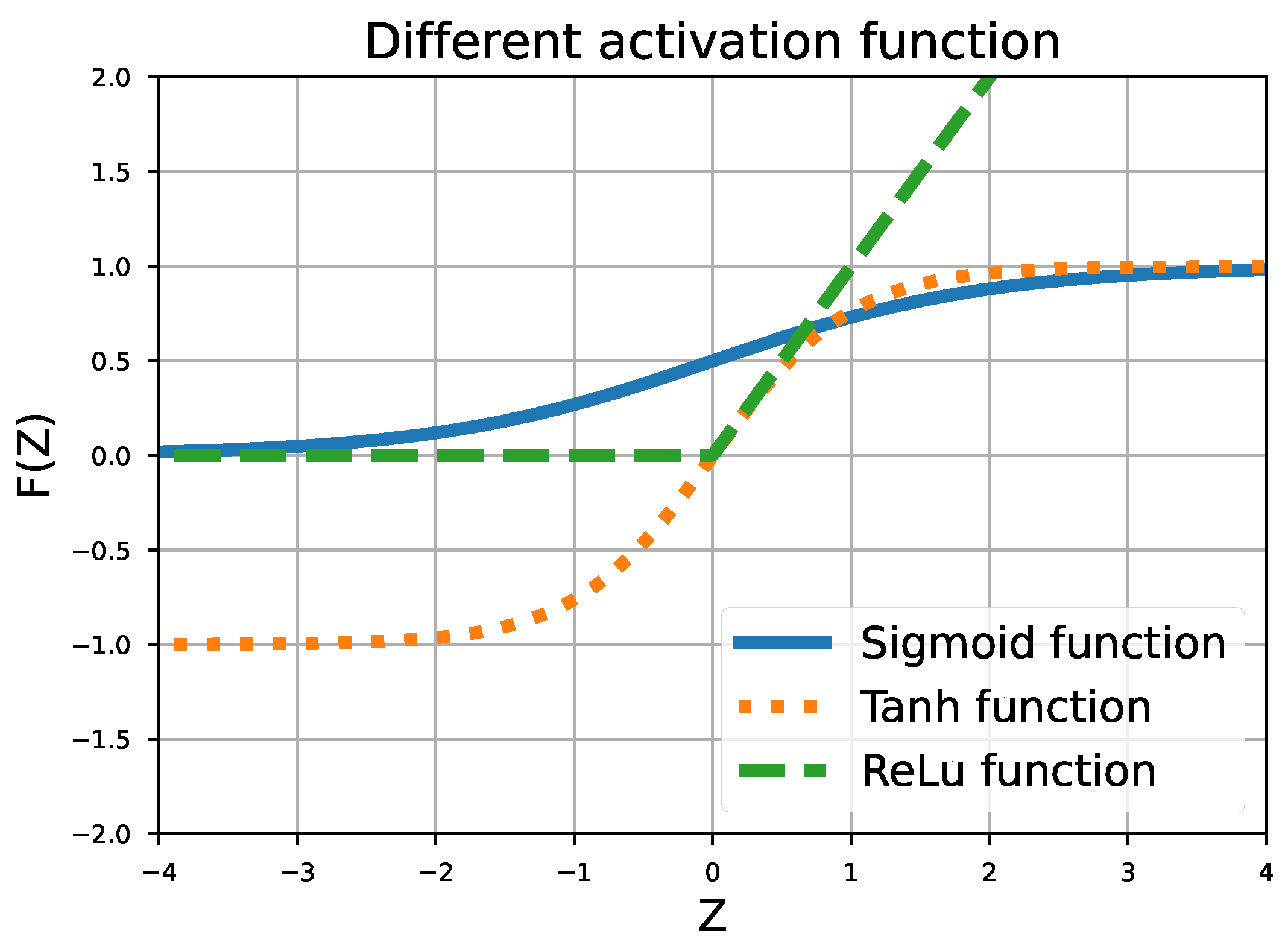
- All architectures containing only “ReLu” layers converge to similar performance, as shown by their comparable performance indicators. The mean R2 score stands around 88%, while the mean MAPE is around 23%. The architecture seems to have minimal impact on the results obtained. Consequently, it is recommended to use less complex network architectures, as more complex ones do not offer significant advantages for databases such as the one presented in this article.
- The architectures with only Tanh or Sigmoid activation function fail to obtain good results in only 1000 epochs. This is largely attributed to the data scale. Specifically, Tanh and Sigmoid functions can only output values ranging from −1 to 1 and 0 to 1, respectively. Given that the VB values are expressed in microns (ranging from 0 to 450 μm), a saturation effect is observed. It is important to note that, even when the VB values are scaled to better suit these architectures, the results do not show any significant improvement over those discussed in the following.
- The optimal architecture is composed of two hidden layers, each with six neurons. The first layer utilizes a Tanh activation function, while the second uses an ReLu activation function. Compared with approaches using only ReLu, this architecture improves the R2 score by an average of 5% and MAPE by 8%.
2.7. Confidence Interval Evaluation
3. Results
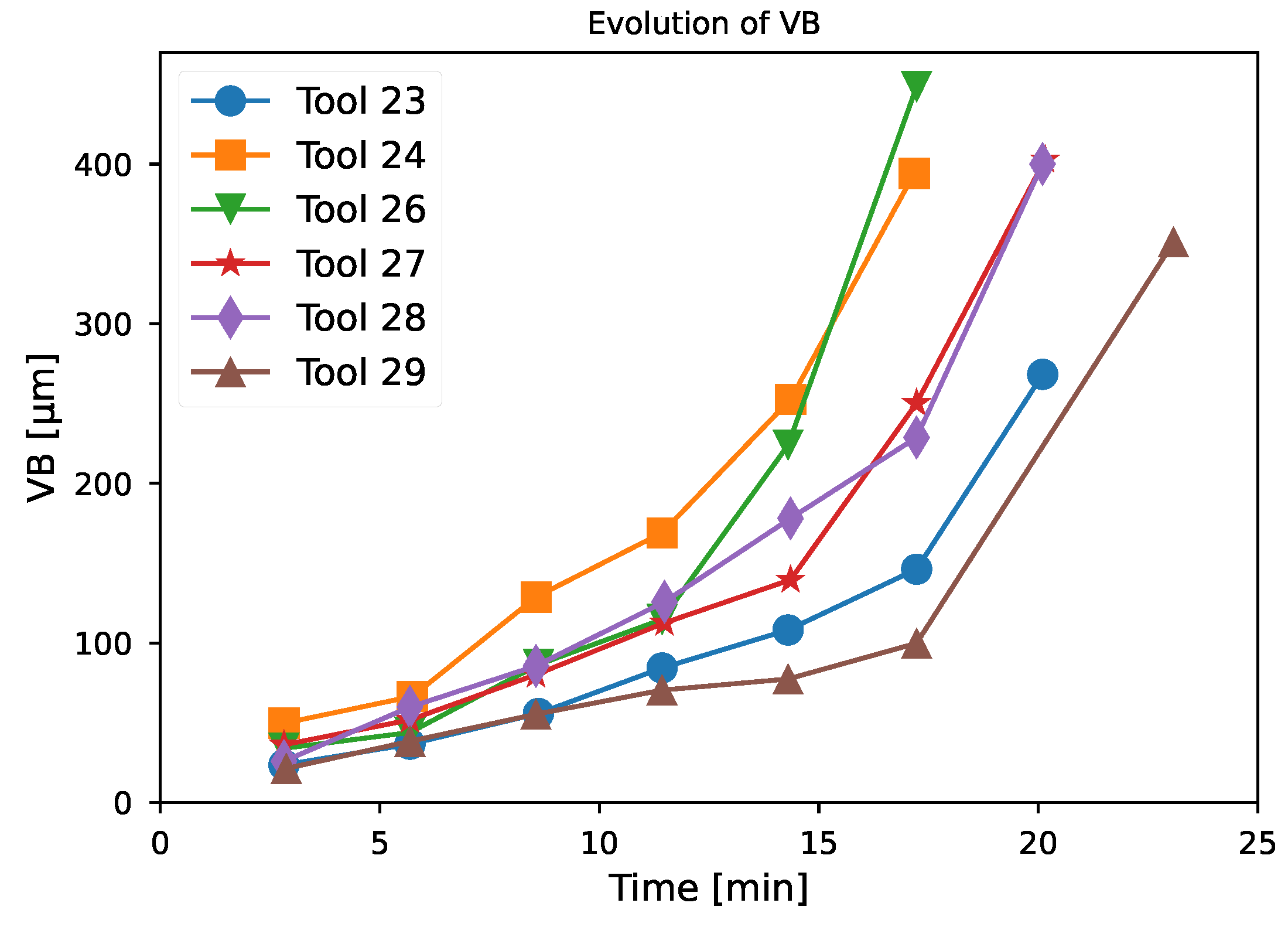
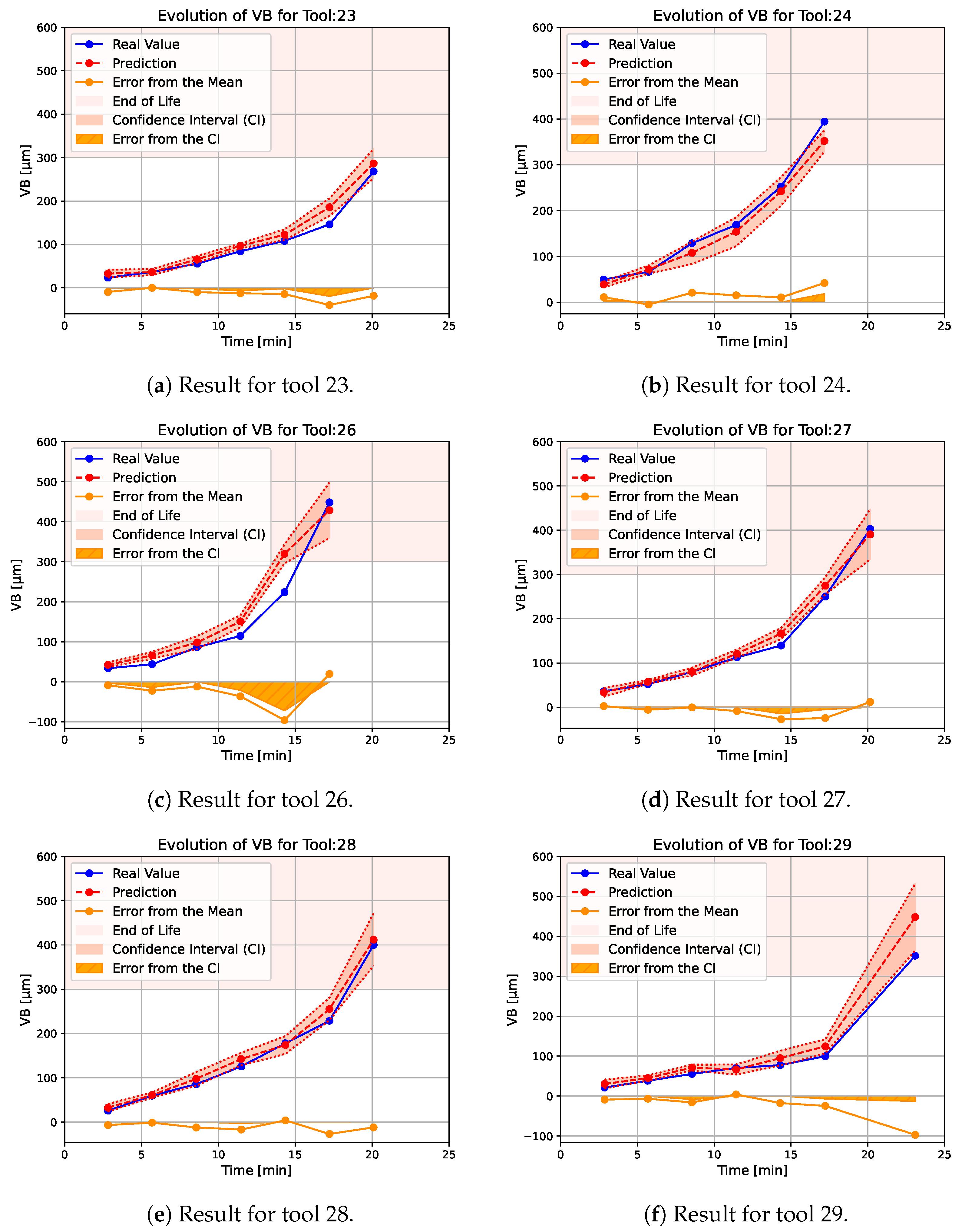
- For tool 23 (Figure 9a), the estimate is consistently slightly higher than the actual observed wear, but the confidence interval almost consistently matches the real value. A more significant overestimation is observed around 17 min that is around 40 μm, but the confidence interval is larger than before and the error on this interval is smaller. For this tool, the end of life has not been reached.
- Compared to the rest of the test database, tool 24 has a higher initial degradation rate. The network estimate has a slightly larger confidence interval over this part of the tool’s life, which is a unique case—generally, the confidence interval increases with time (Figure 9b). Apart from this sudden change in tool wear, the estimator is able to track the degradation correctly, but tends to slightly underestimate the value of the degradation. This is a unique case in this test dataset. For this tool, the observed end of life is reached less than 1 min before the predicted end of life.
- Tool 26 is the tool with the fastest end-of-life degradation (Figure 9c). At the beginning of the tool’s life, the network is able to track the degradation correctly with a relatively low confidence interval; then, due to the sudden change in the wear rate, the estimator strongly overestimates the tool’s degradation. In this case, it even indicates that the tool has reached the end of its life because the prediction around 15 min is higher than 300 μm. Then, the confidence interval increases strongly and the estimate is closer to reality. For this tool, the end of life is reached around 2 min after the predicted end of life.
- The degradation of tools 27 and 28 are fairly similar (Figure 9d,e), there is simply a slightly earlier change in the degradation rate for tool 27 than for tool 28. For both tools, the neural network correctly tracks the degradation and the confidence interval increases slightly at the end of the tool’s life. For these tools, the end of life is reached almost at the same time as the predicted ones.
- Tool 29 has a lower degradation rate than the others and a longer tool life (Figure 9f). The estimator is able to follow the degradation of the tool correctly, but its end of life is overestimated and the confidence interval is significantly larger than for the other tools. For this tool, the end of life is reached 2 min after the predicted end of life.
4. Conclusions
Author Contributions
Funding
Data Availability Statement
Conflicts of Interest
References
- Angseryd, J.; Andrén, H.O. An in-depth investigation of the cutting speed impact on the degraded microstructure of worn PCBN cutting tools. Wear 2011, 271, 2610–2618. [Google Scholar] [CrossRef]
- Klocke, F.; Kuchle, A. Manufacturing Processes; Springer: Berlin/Heidelberg, Germany, 2009; Volume 2, 433p. [Google Scholar] [CrossRef]
- Zaretalab, A.; Haghighi, H.S.; Mansour, S.; Sajadieh, M.S. A mathematical model for the joint optimization of machining conditions and tool replacement policy with stochastic tool life in the milling process. Int. J. Adv. Manuf. Technol. 2018, 96, 2319–2339. [Google Scholar] [CrossRef]
- Baig, R.U.; Javed, S.; Khaisar, M.; Shakoor, M.; Raja, P. Development of an ANN model for prediction of tool wear in turning EN9 and EN24 steel alloy. Adv. Mech. Eng. 2021, 13, 16878140211026720. [Google Scholar] [CrossRef]
- Kuntoğlu, M.; Aslan, A.; Pimenov, D.Y.; Usca, Ü.A.; Salur, E.; Gupta, M.K.; Mikolajczyk, T.; Giasin, K.; Kapłonek, W.; Sharma, S. A review of indirect tool condition monitoring systems and decision-making methods in turning: Critical analysis and trends. Sensors 2020, 21, 108. [Google Scholar] [CrossRef] [PubMed]
- Choudhury, S.K.; Rao, I.A. Optimization of cutting parameters for maximizing tool life. Int. J. Mach. Tools Manuf. 1999, 39, 343–353. [Google Scholar] [CrossRef]
- Wang, X.; Feng, C.X. Development of empirical models for surface roughness prediction in finish turning. Int. J. Adv. Manuf. Technol. 2002, 20, 348–356. [Google Scholar] [CrossRef]
- Wong, T.; Kim, W.; Kwon, P. Experimental support for a model-based prediction of tool wear. Wear 2004, 257, 790–798. [Google Scholar] [CrossRef]
- Equeter, L.; Ducobu, F.; Rivière-Lorphèvre, E.; Serra, R.; Dehombreux, P. An analytic approach to the Cox proportional hazards model for estimating the lifespan of cutting tools. J. Manuf. Mater. Process. 2020, 4, 27. [Google Scholar] [CrossRef]
- Marani, M.; Zeinali, M.; Kouam, J.; Songmene, V.; Mechefske, C.K. Prediction of cutting tool wear during a turning process using artificial intelligence techniques. Int. J. Adv. Manuf. Technol. 2020, 111, 505–515. [Google Scholar] [CrossRef]
- Yang, B.; Lei, Y.; Li, X.; Li, N. Targeted transfer learning through distribution barycenter medium for intelligent fault diagnosis of machines with data decentralization. Expert Syst. Appl. 2024, 244, 122997. [Google Scholar] [CrossRef]
- Gao, K.; Xu, X.; Jiao, S. Measurement and prediction of wear volume of the tool in nonlinear degradation process based on multi-sensor information fusion. Eng. Fail. Anal. 2022, 136, 106164. [Google Scholar] [CrossRef]
- Wang, W.; Liu, W.; Zhang, Y.; Liu, Y.; Zhang, P.; Jia, Z. Precise measurement of geometric and physical quantities in cutting tools inspection and condition monitoring: A review. Chin. J. Aeronaut. 2023, 37, 23–53. [Google Scholar] [CrossRef]
- Bergs, T.; Holst, C.; Gupta, P.; Augspurger, T. Digital image processing with deep learning for automated cutting tool wear detection. Procedia Manuf. 2020, 48, 947–958. [Google Scholar] [CrossRef]
- Yuan, L.; Guo, T.; Qiu, Z.; Fu, X.; Hu, X. An analysis of the focus variation microscope and its application in the measurement of tool parameter. Int. J. Precis. Eng. Manuf. 2020, 21, 2249–2261. [Google Scholar] [CrossRef]
- Siddhpura, A.; Paurobally, R. A review of flank wear prediction methods for tool condition monitoring in a turning process. Int. J. Adv. Manuf. Technol. 2013, 65, 371–393. [Google Scholar] [CrossRef]
- Colantonio, L.; Equeter, L.; Dehombreux, P.; Ducobu, F. Comparison of cutting tool wear classification performance with artificial intelligence techniques. Mater. Res. Proc. 2023, 28, 1265–1274. [Google Scholar] [CrossRef]
- Brito, L.C.; da Silva, M.B.; Duarte, M.A.V. Identification of cutting tool wear condition in turning using self-organizing map trained with imbalanced data. J. Intell. Manuf. 2021, 32, 127–140. [Google Scholar] [CrossRef]
- Brili, N.; Ficko, M.; Klančnik, S. Automatic Identification of Tool Wear Based on Thermography and a Convolutional Neural Network during the Turning Process. Sensors 2021, 21, 1917. [Google Scholar] [CrossRef] [PubMed]
- Pagani, L.; Parenti, P.; Cataldo, S.; Scott, P.J.; Annoni, M. Indirect cutting tool wear classification using deep learning and chip colour analysis. Int. J. Adv. Manuf. Technol. 2020, 111, 1099–1114. [Google Scholar] [CrossRef]
- Ferrando Chacón, J.L.; Fernández de Barrena, T.; García, A.; Sáez de Buruaga, M.; Badiola, X.; Vicente, J. A Novel Machine Learning-Based Methodology for Tool Wear Prediction Using Acoustic Emission Signals. Sensors 2021, 21, 5984. [Google Scholar] [CrossRef]
- Segreto, T.; D’Addona, D.; Teti, R. Tool wear estimation in turning of Inconel 718 based on wavelet sensor signal analysis and machine learning paradigms. Prod. Eng. Res. Devel. 2020, 14, 693–705. [Google Scholar] [CrossRef]
- Colantonio, L.; Equeter, L.; Dehombreux, P.; Ducobu, F. A systematic literature review of cutting tool wear monitoring in turning by using artificial intelligence techniques. Machines 2021, 9, 351. [Google Scholar] [CrossRef]
- Pandiyan, V.; Caesarendra, W.; Tjahjowidodo, T.; Tan, H.H. In-process tool condition monitoring in compliant abrasive belt grinding process using support vector machine and genetic algorithm. J. Manuf. Process. 2018, 31, 199–213. [Google Scholar] [CrossRef]
- Sun, M.; Guo, K.; Zhang, D.; Yang, B.; Sun, J.; Li, D.; Huang, T. A novel exponential model for tool remaining useful life prediction. J. Manuf. Syst. 2024, 73, 223–240. [Google Scholar] [CrossRef]
- Li, H.; Zhang, Z.; Li, T.; Si, X. A review on physics-informed data-driven remaining useful life prediction: Challenges and opportunities. Mech. Syst. Signal Process. 2024, 209, 111120. [Google Scholar] [CrossRef]
- Kim, G.; Yang, S.M.; Kim, D.M.; Kim, S.; Choi, J.G.; Ku, M.; Lim, S.; Park, H.W. Bayesian-based uncertainty-aware tool-wear prediction model in end-milling process of titanium alloy. Appl. Soft Comput. 2023, 148, 110922. [Google Scholar] [CrossRef]
- Khosravi, A.; Nahavandi, S.; Creighton, D.; Atiya, A.F. Comprehensive review of neural network-based prediction intervals and new advances. IEEE Trans. Neural Netw. 2011, 22, 1341–1356. [Google Scholar] [CrossRef] [PubMed]
- Zio, E. A study of the bootstrap method for estimating the accuracy of artificial neural networks in predicting nuclear transient processes. IEEE Trans. Nucl. Sci. 2006, 53, 1460–1478. [Google Scholar] [CrossRef]
- ISO 3685—Tool Life Testing with Single-Point Turning Tools. 1993. Available online: https://www.iso.org/fr/standard/9151.html (accessed on 3 October 2022).
- Seco Tools. Turning Catalog and Technical Guide, 2nd ed.; Seco Tools AB: Fagersta, Sweden, 2018. [Google Scholar]
- Cheng, M.; Jiao, L.; Yan, P.; Jiang, H.; Wang, R.; Qiu, T.; Wang, X. Intelligent tool wear monitoring and multi-step prediction based on deep learning model. J. Manuf. Syst. 2022, 62, 286–300. [Google Scholar] [CrossRef]
- Twardowski, P.; Tabaszewski, M.; Wiciak–Pikuła, M.; Felusiak-Czyryca, A. Identification of tool wear using acoustic emission signal and machine learning methods. Precis. Eng. 2021, 72, 738–744. [Google Scholar] [CrossRef]
- Welch, P. The use of fast Fourier transform for the estimation of power spectra: A method based on time averaging over short, modified periodograms. IEEE Trans. Audio Electroacoust. 1967, 15, 70–73. [Google Scholar] [CrossRef]
- Bishara, A.J.; Hittner, J.B. Testing the significance of a correlation with nonnormal data: Comparison of Pearson, Spearman, transformation, and resampling approaches. Psychol. Methods 2012, 17, 399. [Google Scholar] [CrossRef]
- Wilcox, R.R. Comparing Pearson correlations: Dealing with heteroscedasticity and nonnormality. Commun. Stat.-Simul. Comput. 2009, 38, 2220–2234. [Google Scholar] [CrossRef]
- Kilundu, B.; Dehombreux, P.; Chiementin, X. Tool wear monitoring by machine learning techniques and singular spectrum analysis. Mech. Syst. Signal Process. 2011, 25, 400–415. [Google Scholar] [CrossRef]
- Xu, C.; Dou, J.; Chai, Y.; Li, H.; Shi, Z.; Xu, J. The relationships between cutting parameters, tool wear, cutting force and vibration. Adv. Mech. Eng. 2018, 10, 1687814017750434. [Google Scholar] [CrossRef]
- Lee, L.C.; Lee, K.S.; Gan, C.S. On the correlation between dynamic cutting force and tool wear. Int. J. Mach. Tools Manuf. 1989, 29, 295–303. [Google Scholar] [CrossRef]
- Bejani, M.M.; Ghatee, M. A systematic review on overfitting control in shallow and deep neural networks. Artif. Intell. Rev. 2021, 54, 6391–6438. [Google Scholar] [CrossRef]
- Keras. Open Source API. Available online: https://keras.io/ (accessed on 24 May 2024).
- Tiwari, M.K.; Chatterjee, C. Uncertainty assessment and ensemble flood forecasting using bootstrap-based artificial neural networks (BANNs). J. Hydrol. 2010, 382, 20–33. [Google Scholar] [CrossRef]
- Chambers, J.M.; Cleveland, W.S.; Kleiner, B.; Tukey, P.A. Graphical Methods for Data Analysis; Chapman and Hall/CRC: Boca Raton, FL, USA, 2018. [Google Scholar] [CrossRef]


| Test N° | Material | Cutting Speed— [m/min] | Feed [mm/rev] | Depth of Cut [mm] |
|---|---|---|---|---|
| 1 to 10 | C45 | 260 | 0.2 | 1 |
| 11 to 15 | C45 | 250 | 0.2 | 1 |
| 16 | C45 | 240 | 0.2 | 1 |
| 17 to 20 | C45 | 265 | 0.2 | 1 |
| 21 to 30 | C45 | Variable: 240 to 260 | 0.2 | 1 |
| Parameters Measured | Associated Variables |
|---|---|
| Cutting force and Torque | , , , , and |
| Time | Machining time |
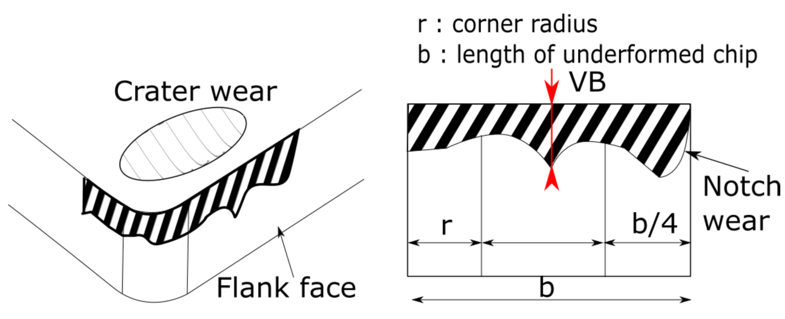
| Picture of the tool | VB and notch wear |
| Feature Processing Method | Mathematical Equation |
|---|---|
| Mean () | |
| Standard deviation () | |
| Skewness (skew) | |
| Kurtosis (kurt) | |
| Root Mean Square (RMS) |
| Features | Spearman’s Correlation Coefficient with Respect to VB |
|---|---|
| 0.89 | |
| 0.87 | |
| Machining duration | 0.84 |
| total machined length | 0.84 |
| 0.79 |
| Version | Task |
|---|---|
| Python 3.8.11 | Programming language |
| Keras 2.4.3 | NN API |
| Tensorflow 2.3.0 | Open source platform for machine learning |
| Matplotlib 3.4.2 | Visualization |
| Pandas 1.2.5 | Data manipulation |
| Scipy 1.6.2 | Mathematical computation |
| Numpy 1.22.3 | Array manipulation |
| Network Architecture | MSE | R2 Score | MAPE | Activation Function |
|---|---|---|---|---|
| [5, 6, 6, 1] | 850 | 94.5% | 15% | Tanh and ReLu |
| [5, 6, 10, 6, 1] | 1200 | 91% | 19% | Tanh, ReLu and ReLu |
| [5, 6, 6, 1] | 1250 | 90% | 25% | Sigmoid and ReLu |
| [5, 5, 13, 9, 1] | 1330 | 90% | 23% | All ReLu |
| [5, 11, 1] | 1550 | 89% | 22% | All ReLu |
| [5, 6, 1] | 1600 | 88% | 27% | All ReLu |
| [5, 12, 5, 1] | 1630 | 88% | 25% | All ReLu |
| [5, 6, 6, 1] | 1700 | 87% | 26% | All ReLu |
| [5, 6, 6, 1] | 12,000 | 14% | 30% | All Tanh |
| [5, 6, 6, 1] | 12,000 | 14% | 30% | All Sigmoid |
Disclaimer/Publisher’s Note: The statements, opinions and data contained in all publications are solely those of the individual author(s) and contributor(s) and not of MDPI and/or the editor(s). MDPI and/or the editor(s) disclaim responsibility for any injury to people or property resulting from any ideas, methods, instructions or products referred to in the content. |
© 2024 by the authors. Licensee MDPI, Basel, Switzerland. This article is an open access article distributed under the terms and conditions of the Creative Commons Attribution (CC BY) license (https://creativecommons.org/licenses/by/4.0/).
Share and Cite
Colantonio, L.; Equeter, L.; Dehombreux, P.; Ducobu, F. Confidence Interval Estimation for Cutting Tool Wear Prediction in Turning Using Bootstrap-Based Artificial Neural Networks. Sensors 2024, 24, 3432. https://doi.org/10.3390/s24113432
Colantonio L, Equeter L, Dehombreux P, Ducobu F. Confidence Interval Estimation for Cutting Tool Wear Prediction in Turning Using Bootstrap-Based Artificial Neural Networks. Sensors. 2024; 24(11):3432. https://doi.org/10.3390/s24113432
Chicago/Turabian StyleColantonio, Lorenzo, Lucas Equeter, Pierre Dehombreux, and François Ducobu. 2024. "Confidence Interval Estimation for Cutting Tool Wear Prediction in Turning Using Bootstrap-Based Artificial Neural Networks" Sensors 24, no. 11: 3432. https://doi.org/10.3390/s24113432
APA StyleColantonio, L., Equeter, L., Dehombreux, P., & Ducobu, F. (2024). Confidence Interval Estimation for Cutting Tool Wear Prediction in Turning Using Bootstrap-Based Artificial Neural Networks. Sensors, 24(11), 3432. https://doi.org/10.3390/s24113432