
Electrical Sensor Calibration by Fuzzy Clustering with Mandatory Constraint


Abstract
1. Introduction
2. Related Work
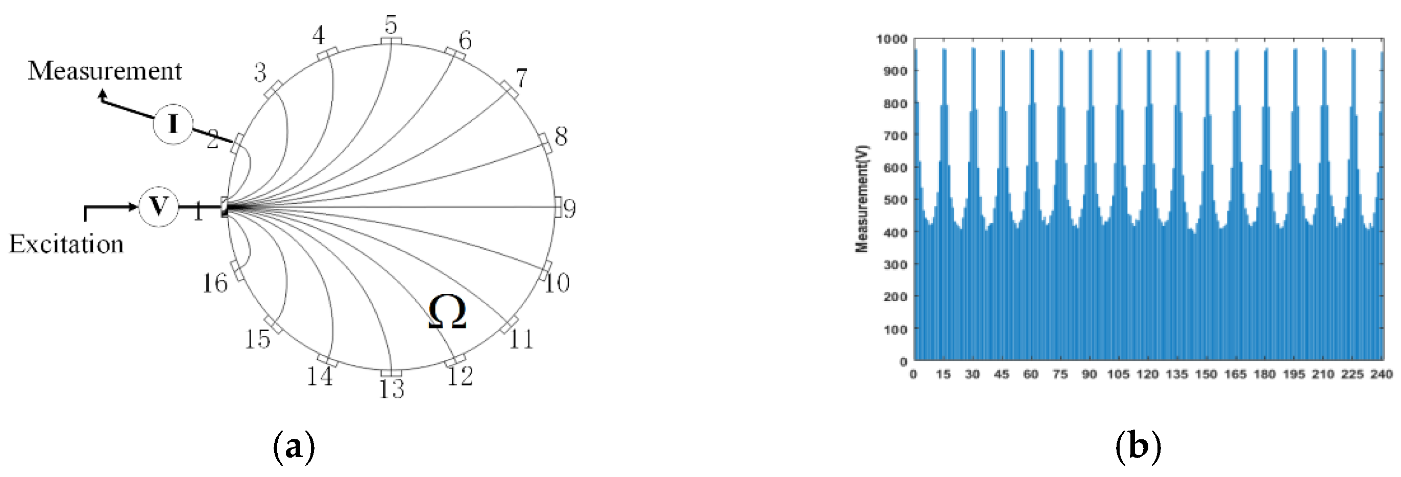
2.1. ETS and SPF Calculation
2.2. FCM Clustering Algorithm
| Algorithm 1. The FCM algorithm. |
| Input: Dataset S, the number of clusters c, exponent indexes m, and acceptable error ε Output: The clustering label of each datum in S |
| Method: (1) Initialize all clustering centers in FCM as v1, v2, …, vc; (2) Problem 1: Fix vi and solve uij by the first formula in Equation (8), i = 1~c, j = 1~n; (3) Problem 2: Fix uij and solve vi using the second formula in Equation (8), i = 1~c; (4) Stop if the difference of the partition matrix at the tth iteration satisfies ||Ut+1-Ut|| ≤ ε and go to Step (5); otherwise, go to Step (2); (5) Partition S into c clusters: C1, C2, …, Cc by the fuzzy membership degrees of all data. |
3. Mandatory Constraint-Based Fuzzy Clustering for Decreasing Error in Inaccurate Data
3.1. Three Types of Calibration Data
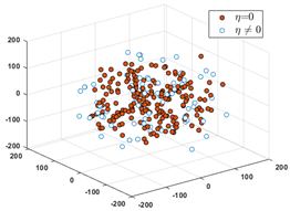
3.2. Cluster Characteristics of Sample Data
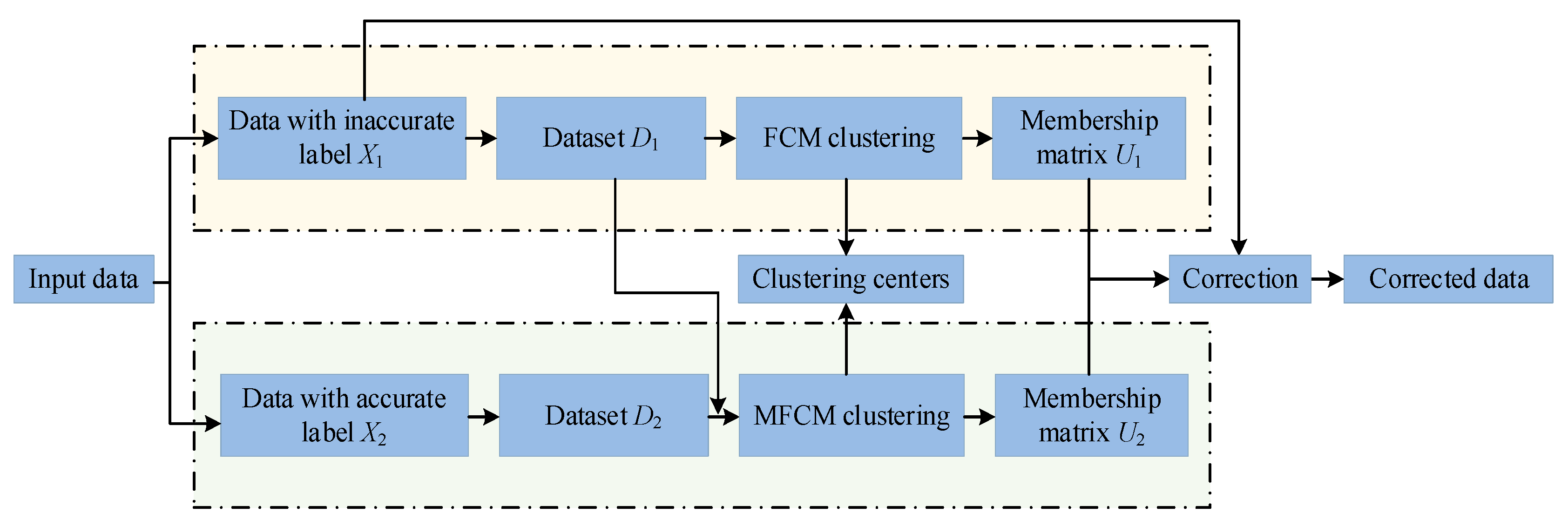
3.3. Mandatory Constraint Fuzzy Clustering for Calibration
4. Experimental Section
4.1. Experimental Platform and Measuring Condition
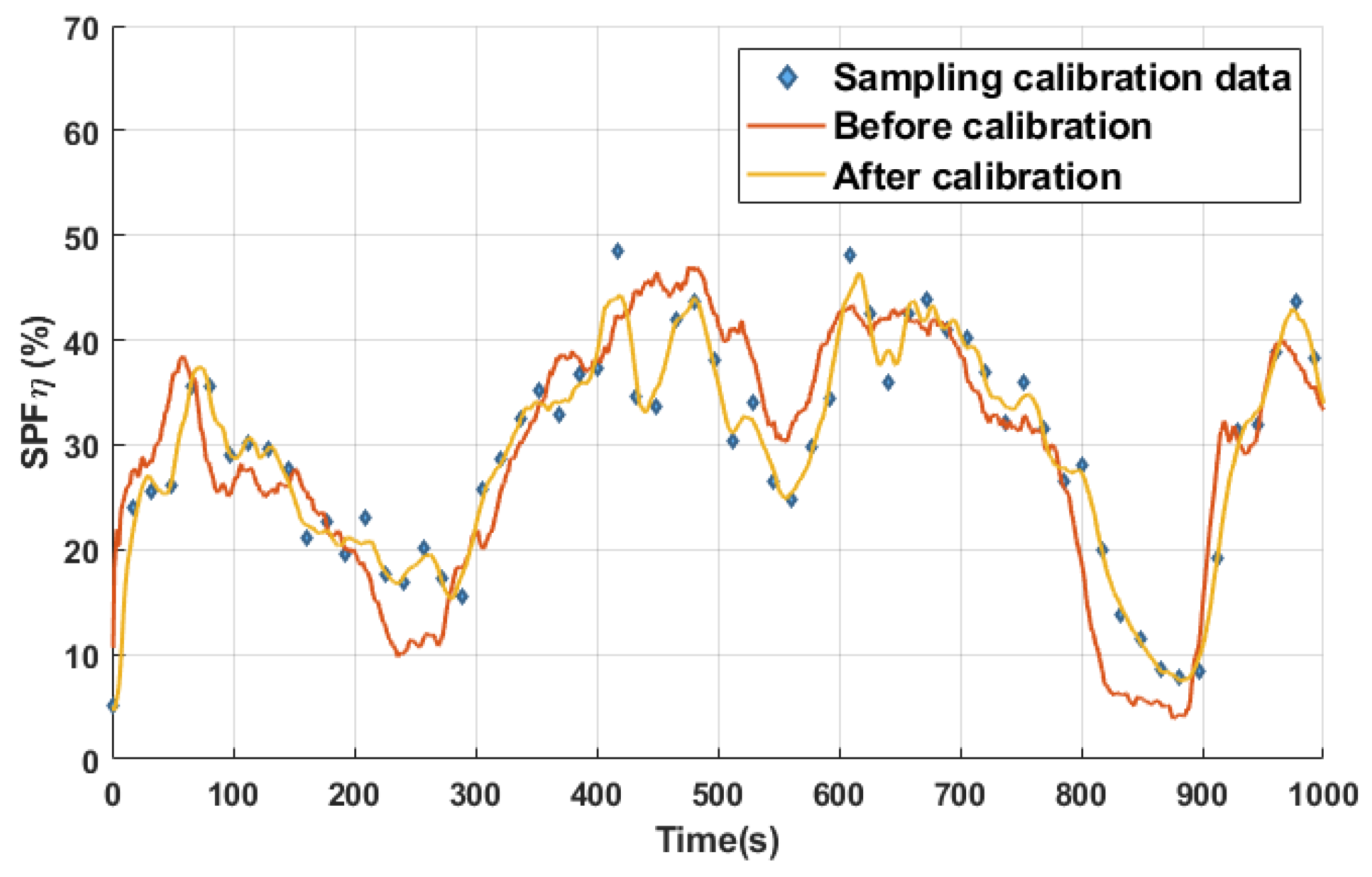
4.2. Experimental Results and Analysis
5. Conclusions
Author Contributions
Funding
Institutional Review Board Statement
Informed Consent Statement
Data Availability Statement
Conflicts of Interest
References
- Berger, M.; Schott, C.; Close, G. Bayesian Sensor Calibration of a CMOS-Integrated Hall Sensor Against Thermomechanical Cross-Sensitivities. IEEE Sens. J. 2023, 23, 6976–6989. [Google Scholar] [CrossRef]
- Bulot, F.M.; Ossont, S.J.; Morris, A.K.; Basford, P.J.; Easton, N.H.; Mitchell, H.L.; Loxham, M. Characterisation and calibration of low-cost PM sensors at high temporal resolution to reference-grade performance. Heliyon 2023, 9, e15943. [Google Scholar] [CrossRef] [PubMed]
- Munz, H.; Ingwersen, J.; Streck, T. On-Site Sensor Calibration Procedure for Quality Assurance of Barometric Process Separation (BaPS) Measurements. Sensors 2023, 23, 4615. [Google Scholar] [CrossRef] [PubMed]
- Grammenos, A.; Mascolo, C.; Crowcroft, J. You Are Sensing, but Are You Biased? A User Unaided Sensor Calibration Approach for Mobile Sensing. Proc. ACM Interact. Mob. Wearable Ubiquitous Technol. 2018, 2, 1–26. [Google Scholar] [CrossRef]
- Zaidan, M.A.; Motlagh, N.H.; Fung, P.L.; Khalaf, A.S.; Matsumi, Y.; Ding, A.; Hussein, T. Intelligent Air Pollution Sensors Calibration for Extreme Events and Drifts Monitoring. IEEE Trans. Indust. Inf. 2023, 19, 1366–1379. [Google Scholar] [CrossRef]
- Soto-Marchena, D.; Barrero, F.; Colodro, F.; Arahal, M.R.; Mora, J.L. On-Site Calibration of an Electric Drive: A Case Study Using a Multiphase System. Sensors 2023, 23, 7317. [Google Scholar] [CrossRef] [PubMed]
- Liu, W.; Liang, B.; Jia, Z.; Feng, D.; Jiang, X.; Li, X.; Zhou, M. High-Accuracy Calibration Based on Linearity Adjustment for Eddy Current Displacement Sensor. Sensors 2018, 18, 2842. [Google Scholar] [CrossRef]
- Halter, R.; Hartov, A.; Paulsen, K. Design and implementation of a high frequency electrical impedance tomography system. Physiol. Meas. 2004, 25, 379–388. [Google Scholar] [CrossRef]
- Wang, Z.; Yue, S.; Wang, H.; Wang, Y. Data preprocessing methods for electrical impedance tomography: A review. Phyl. Meas. 2020, 41, 093–102. [Google Scholar] [CrossRef]
- Smith, R.W.; Freeston, I.L.; Brown, B.H. A real-time electrical impedance tomography system for clinical use-design and preliminary results. IEEE Trans. Biomed. Eng. 1995, 42, 133–140. [Google Scholar] [CrossRef]
- Tan, Y.; Yue, S. Solid concentration estimation by Kalman filter. Sensors 2020, 20, 2657. [Google Scholar] [CrossRef]
- Wu, J.; Yue, S.; Ma, H. An experimental device for calibration of concentration and velocity of two-phase flow based on electrical impedance measurement system. Proc. IEEE Instr. Meas. 2021, 56, 125–131. [Google Scholar]
- Kolodner, J. Case-Based Reasoning; Morgan Kaufmann Publisher: Burlington, MA, USA, 1993. [Google Scholar]
- Yue, S.; Wang, J.; Tao, G.; Wang, H. An unsupervised grid-based approach for clustering analysis. Sci. China Inf. Sci. 2010, 53, 1345–1357. [Google Scholar] [CrossRef]
- Yang, L.; Yue, S.; Tan, Y. Solid component fraction in multi-phase flows using electrical resistance tomography and kalman filter. Proc. IEEE Instr. Meas. 2020, 55, 1367–1374. [Google Scholar]
- Xu, R.; Wunsch, D. Survey of clustering algorithms. IEEE Trans. Neural Netw. 2005, 16, 645–678. [Google Scholar] [CrossRef] [PubMed]
- Bezdek, J.C. Fuzzy Models for Pattern Recognition; Plenum Press: New York, NY, USA, 1992. [Google Scholar]
- Tan, Y.; Yue, S. ERT based computation of solid phase fraction in solid-liquid flow with various object sizes. IEEE Access 2022, 10, 98441–98449. [Google Scholar] [CrossRef]
- Sohal, H.; Wi, H.; McEwan, A.L.; Woo, E.J.; Oh, T.I. Electrical impedance imaging system using FPGAs for flexibility and interoperability. Biomed. Eng. 2014, 13, 126–133. [Google Scholar] [CrossRef] [PubMed]
- Anderson, D.; Zare, A.; Price, S. Comparing fuzzy, probabilistic, and possibilistic partitions using the earth mover’s distance. IEEE Trans. Fuzzy Syst. 2013, 21, 766–775. [Google Scholar] [CrossRef]
- Carter, M.W.; Price, C.C. Operations Research; CRC Press Inc.: Boca Raton, FL, USA, 2000. [Google Scholar]
- Wang, Z.; Wang, S.S.; Bai, L.; Wang, W.S.; Shao, Y.H. Semi-supervised fuzzy clustering with fuzzy pairwise constraints. IEEE Trans. Fuzzy Syst. 2022, 30, 3797–3811. [Google Scholar] [CrossRef]
- Yue, S.; Wang, J.; Bao, X. A new validity index for evaluating the clustering results by partitional clustering algorithms. Soft Comput. 2016, 20, 1127–1138. [Google Scholar] [CrossRef]
- Borg, I.; Groenen, P. Modern Multidimensional Scaling: Theory and Applications; Springer Series in Statistics: Berlin/Heidelberg, Germany, 2005. [Google Scholar]
- Wang, Q.; Heng, Z. Near MDS codes from oval polynomials. Discr. Math. 2021, 10, 344–352. [Google Scholar] [CrossRef]
- Wang, Z.; Yue, S.; Li, Q.; Liu, X.; Wang, H.; McEwan, A. Unsupervised evaluation and optimization for electrical impedance tomography. IEEE Tran. Instr. Meas. 2021, 70, 4506312. [Google Scholar] [CrossRef]
- Lukas, M.A. Robust generalized cross-validation for choosing the regularization parameter. Inverse Prob. 2006, 22, 1883–1902. [Google Scholar] [CrossRef]


| 0 | [0.01, 0.10] | [0.11, 0.20] |
 Dominant rate of SPF: 61.56% | 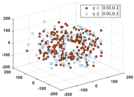 Dominant rate of SPF: 72.73% |  Dominant rate of SPF: 58.19% |
| [0.21, 0.30] | [0.31, 0.40] | [0.41, 1.00] |
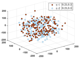 Dominant rate of SPF: 66.27% |  Dominant rate of SPF: 48.62% | 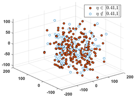 Dominant rate of SPF: 51.08% |
| SPF Interval | 0 | [0, 0.10] | [0.11, 0.20] | [0.21, 0.30] | [0.31, 0.40] | [0.41, 1.00] |
|---|---|---|---|---|---|---|
| Noncorrected | 61.56% | 72.73% | 58.19% | 66.27% | 48.62% | 51.08% |
| Corrected | 72.19% | 79.49% | 68.04% | 72.16% | 60.94% | 58.35% |
| SPF(%) | 0~5 | 6~10 | 11~15 | 16~20 | 21~25 | 25~29 | Total |
|---|---|---|---|---|---|---|---|
| Number | 7000 | 7000 | 7000 | 7000 | 7000 | 7000 | 42,000 |
| Index | RMSE | MAE | MAPE | R2 | |
|---|---|---|---|---|---|
| LPM | Noncorrected | 2.6804 | 2.0141 | 142.36% | 74.56% |
| Corrected | 1.8247 | 1.3137 | 62.65% | 88.93% | |
Disclaimer/Publisher’s Note: The statements, opinions and data contained in all publications are solely those of the individual author(s) and contributor(s) and not of MDPI and/or the editor(s). MDPI and/or the editor(s) disclaim responsibility for any injury to people or property resulting from any ideas, methods, instructions or products referred to in the content. |
© 2024 by the authors. Licensee MDPI, Basel, Switzerland. This article is an open access article distributed under the terms and conditions of the Creative Commons Attribution (CC BY) license (https://creativecommons.org/licenses/by/4.0/).
Share and Cite
Yue, S.; Fu, K.; Liu, L.; Zhao, Y. Electrical Sensor Calibration by Fuzzy Clustering with Mandatory Constraint. Sensors 2024, 24, 3068. https://doi.org/10.3390/s24103068
Yue S, Fu K, Liu L, Zhao Y. Electrical Sensor Calibration by Fuzzy Clustering with Mandatory Constraint. Sensors. 2024; 24(10):3068. https://doi.org/10.3390/s24103068
Chicago/Turabian StyleYue, Shihong, Keyi Fu, Liping Liu, and Yuwei Zhao. 2024. "Electrical Sensor Calibration by Fuzzy Clustering with Mandatory Constraint" Sensors 24, no. 10: 3068. https://doi.org/10.3390/s24103068
APA StyleYue, S., Fu, K., Liu, L., & Zhao, Y. (2024). Electrical Sensor Calibration by Fuzzy Clustering with Mandatory Constraint. Sensors, 24(10), 3068. https://doi.org/10.3390/s24103068