
Automatic Localization of Soybean Seedlings Based on Crop Signaling and Multi-View Imaging


Abstract
1. Introduction
2. Materials and Methods
2.1. Seed Treatment and Seedling Culture
2.2. Acquisition of Fluorescence Images
2.3. Image Pre-Processing and Pseudo-Color Image Generation
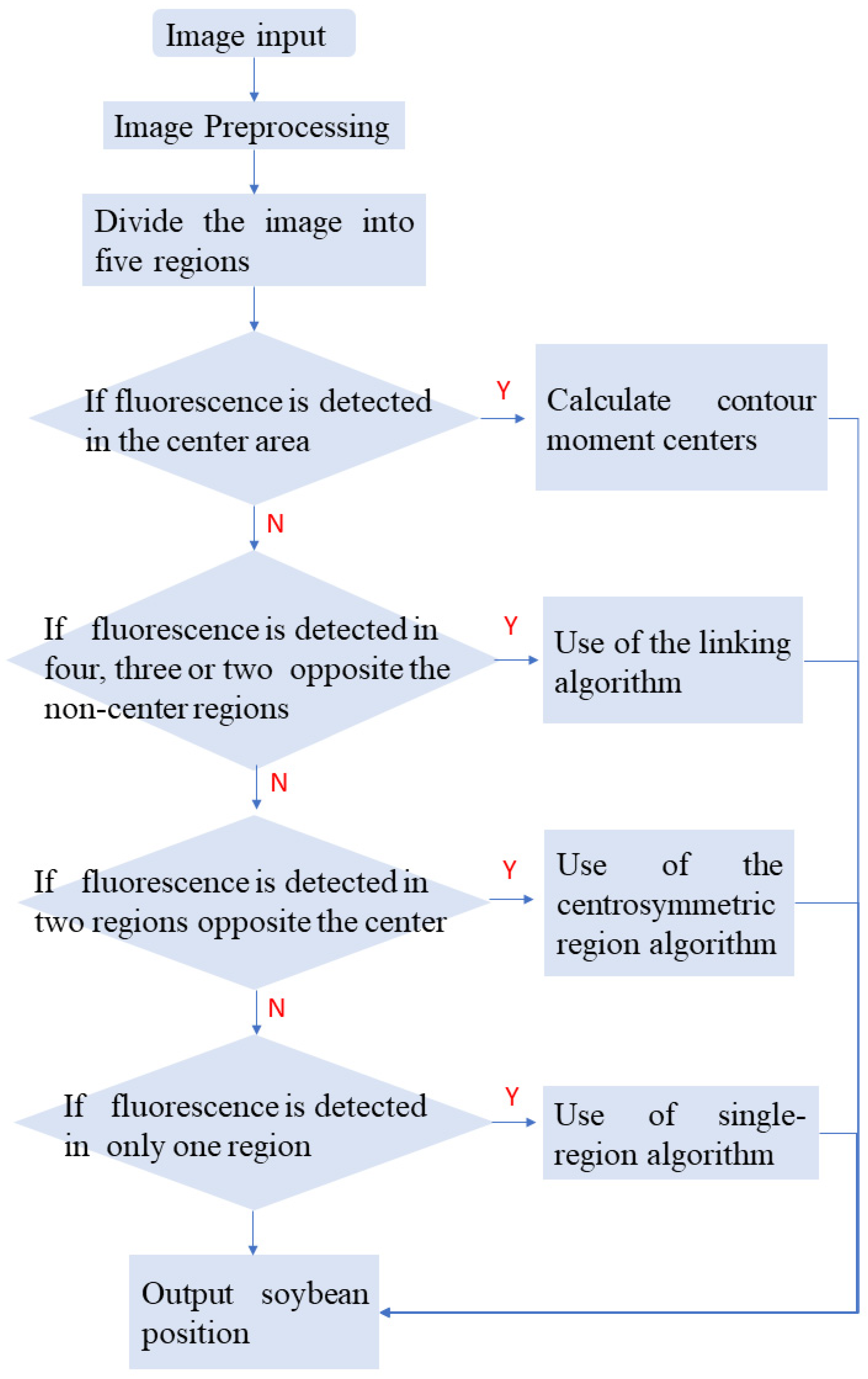
2.4. Improved Multi-View Positioning Algorithm
2.5. Statical Analysis
3. Results
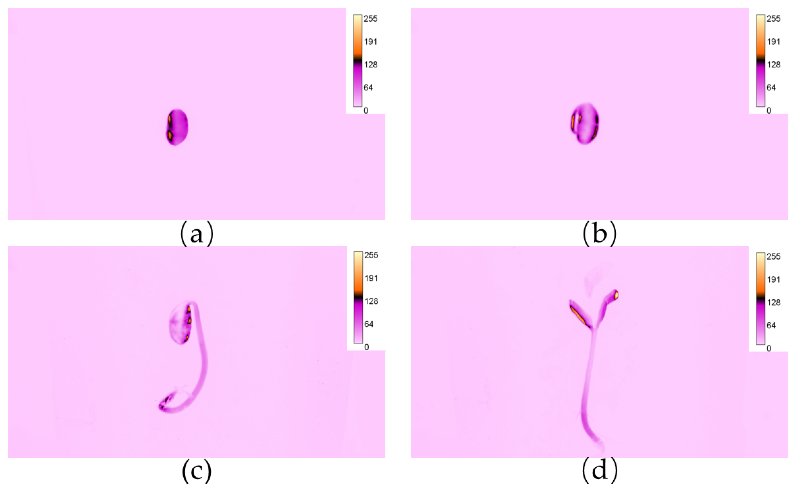
3.1. Visibility and Distribution of Rh-B Fluorescence in Soybean
3.2. Effects of Different Rh-B Concentrations and Different Soaking Times on the Fluorescence Visibility of Soybean Seedlings
3.3. Effects of Rh-B Treatment on the Growth of Soybean Plants
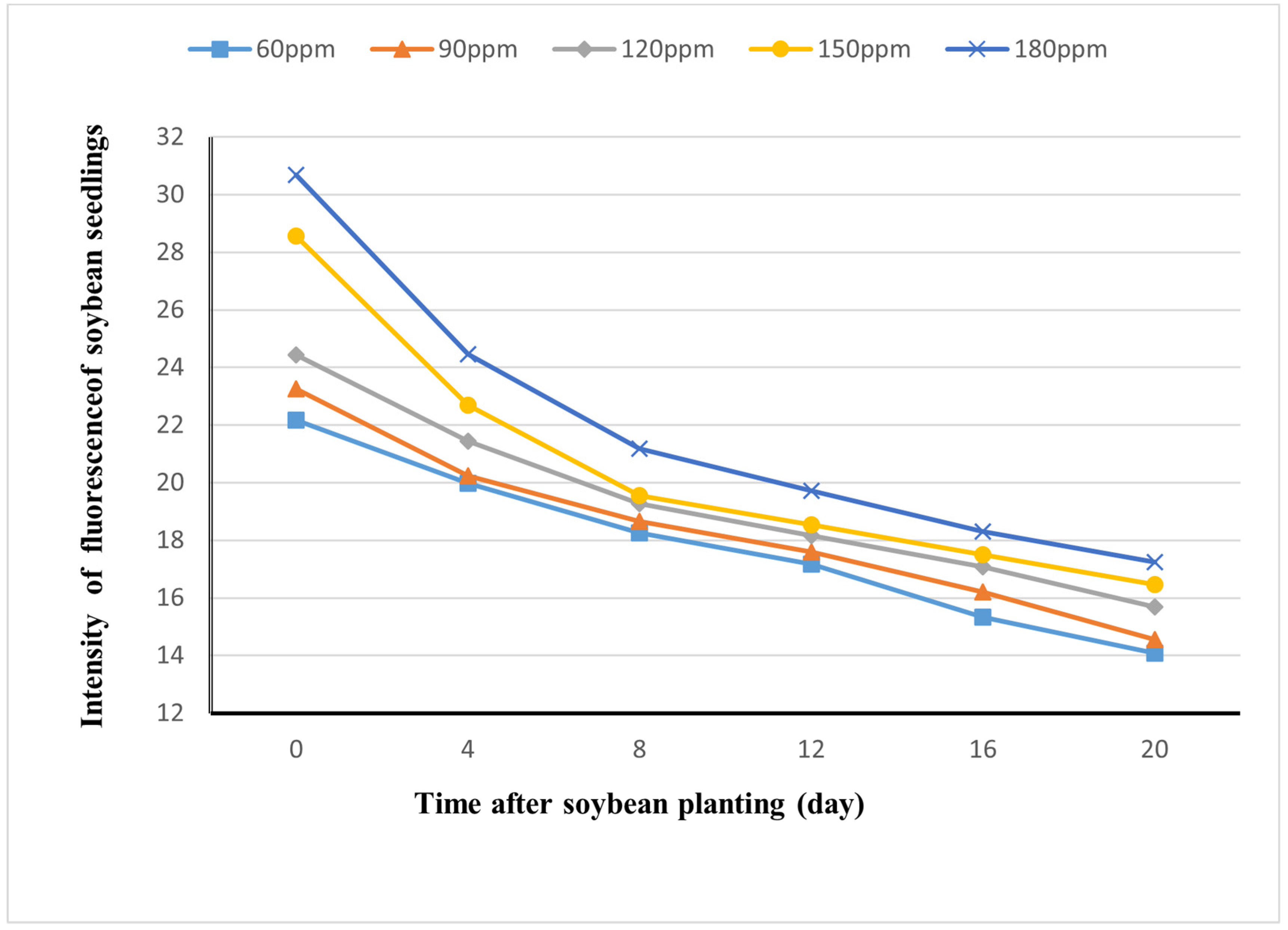
3.4. Decay of Visibility of Rh-B Fluorescence in Soybean
3.5. Result of Identification and Location of Soybean Plants
4. Discussion
5. Conclusions
Author Contributions
Funding
Institutional Review Board Statement
Informed Consent Statement
Data Availability Statement
Conflicts of Interest
References
- Ferreir, A.D.S.; Freitas, D.M.; da Silva, G.G.; Pistori, H.; Folhes, M.T. Weed detection in soybean crops using ConvNets. Comput. Electron. Agric. 2017, 143, 314–324. [Google Scholar] [CrossRef]
- Ahmed, S.; Kumar, V.; Alam, M.; Dewan, M.R.; Bhuiyan, K.A.; Miajy, A.A.; Saha, A.; Singh, S.; Timsina, J.; Krupnik, T.J. Integrated weed management in transplanted rice: Options for addressing labor constraints and improving farmers’ income in Bangladesh. Weed Technol. 2021, 35, 697–709. [Google Scholar] [CrossRef]
- Bakhshipour, A.; Jafari, A.; Nassiri, S.M.; Zare, D. Weed segmentation using texture features extracted from wavelet sub-images. Biosyst. Eng. 2017, 157, 1–12. [Google Scholar] [CrossRef]
- Chang, C.-L.; Xie, B.-X.; Chung, S.-C. Mechanical control with a deep learning method for precise weeding on a farm. Agriculture 2021, 11, 1049. [Google Scholar] [CrossRef]
- Dai, X.; Xu, Y.; Zheng, J.; Song, H. Analysis of the variability of pesticide concentration downstream of inline mixers for direct nozzle injection systems. Biosyst. Eng. 2019, 180, 59–69. [Google Scholar] [CrossRef]
- Fan, X.; Chai, X.; Zhou, J.; Sun, T. Deep learning based weed detection and target spraying robot system at seedling stage of cotton field. Comput. Electron. Agric. 2023, 214, 108317. [Google Scholar] [CrossRef]
- Fennimore, S.A.; Slaughter, D.C.; Siemens, M.C.; Leon, R.G.; Saber, M.N. Technology for automation of weed control in specialty crops. Weed Technol. 2016, 30, 823–837. [Google Scholar] [CrossRef]
- Gaur, M.; Faldu, K.; Sheth, A. Semantics of the black-box: Can knowledge graphs help make deep learning systems more interpretable and explainable? IEEE Internet Comput. 2021, 25, 51–59. [Google Scholar] [CrossRef]
- Grassini, P.; La Menza, N.C.; Edreira, J.I.R.; Monzón, J.P.; Tenorio, F.A.; Specht, J.E. Soybean. In Crop Physiology Case Histories for Major Crops; Elsevier: Amsterdam, The Netherlands, 2021; pp. 282–319. [Google Scholar]
- Hasan, A.M.; Sohel, F.; Diepeveen, D.; Laga, H.; Jones, M.G. A survey of deep learning techniques for weed detection from images. Comput. Electron. Agric. 2021, 184, 106067. [Google Scholar] [CrossRef]
- He, D.; Qiao, Y.; Li, P.; Gao, Z.; Li, H.; Tang, J. Weed recognition based on SVM-DS multi-feature fusion. Nongye Jixie Xuebao = Trans. Chin. Soc. Agric. Mach. 2013, 44, 182–187. [Google Scholar]
- Jugulam, M.; Shyam, C. Non-target-site resistance to herbicides: Recent developments. Plants 2019, 8, 417. [Google Scholar] [CrossRef] [PubMed]
- Li, B.; Wang, G.; Fan, C.; Su, L.; Xu, X. Effects of different tillage methods on weed emergence in summer soybean field. J. Hebei Agric. Sci 2009, 3, 28–30. [Google Scholar]
- Li, Y.; Guo, Z.; Shuang, F.; Zhang, M.; Li, X. Key technologies of machine vision for weeding robots: A review and benchmark. Comput. Electron. Agric. 2022, 196, 106880. [Google Scholar] [CrossRef]
- Liu, B.; Bruch, R. Weed detection for selective spraying: A review. Curr. Robot. Rep. 2020, 1, 19–26. [Google Scholar] [CrossRef]
- Liu, K.; Liu, K. Chemistry and nutritional value of soybean components. In Soybeans: Chemistry, Technology, and Utilization; Springer: New York, NY, USA, 1997; pp. 25–113. [Google Scholar]
- Mattivi, P.; Pappalardo, S.E.; Nikolić, N.; Mandolesi, L.; Persichetti, A.; De Marchi, M.; Masin, R. Can commercial low-cost drones and open-source GIS technologies be suitable for semi-automatic weed mapping for smart farming? A case study in NE Italy. Remote Sens. 2021, 13, 1869. [Google Scholar] [CrossRef]
- Melander, B.; Rasmussen, G. Effects of cultural methods and physical weed control on intrarow weed numbers, manual weeding and marketable yield in direct-sown leek and bulb onion. Weed Res. 2001, 41, 491–508. [Google Scholar] [CrossRef]
- Nguyen, T.T.; Slaughter, D.C.; Fennimore, S.A.; Vuong, V.L. Designing and evaluating the use of crop signaling markers for fully automated and robust weed control technology. In Proceedings of the 2017 ASABE Annual International Meeting, Spokane, WA, USA, 16–19 July 2017; American Society of Agricultural and Biological Engineers: St. Joseph, MI, USA, 2017; p. 1. [Google Scholar]
- Onyango, C.M.; Marchant, J. Segmentation of row crop plants from weeds using colour and morphology. Comput. Electron. Agric. 2003, 39, 141–155. [Google Scholar] [CrossRef]
- Rai, N.; Zhang, Y.; Villamil, M.; Howatt, K.; Ostlie, M.; Sun, X. Agricultural weed identification in images and videos by integrating optimized deep learning architecture on an edge computing technology. Comput. Electron. Agric. 2024, 216, 108442. [Google Scholar] [CrossRef]
- Raja, R.; Nguyen, T.T.; Slaughter, D.C.; Fennimore, S.A. Real-time robotic weed knife control system for tomato and lettuce based on geometric appearance of plant labels. Biosyst. Eng. 2020, 194, 152–164. [Google Scholar] [CrossRef]
- Raja, R.; Nguyen, T.T.; Slaughter, D.C.; Fennimore, S.A. Real-time weed-crop classification and localisation technique for robotic weed control in lettuce. Biosyst. Eng. 2020, 192, 257–274. [Google Scholar] [CrossRef]
- Raja, R.; Nguyen, T.T.; Vuong, V.L.; Slaughter, D.C.; Fennimore, S.A. RTD-SEPs: Real-time detection of stem emerging points and classification of crop-weed for robotic weed control in producing tomato. Biosyst. Eng. 2020, 195, 152–171. [Google Scholar] [CrossRef]
- Raja, R.; Slaughter, D.C.; Fennimore, S.A.; Nguyen, T.T.; Vuong, V.L.; Sinha, N.; Tourte, L.; Smith, R.F.; Siemens, M.C. Crop signalling: A novel crop recognition technique for robotic weed control. Biosyst. Eng. 2019, 187, 278–291. [Google Scholar] [CrossRef]
- Raja, R.; Slaughter, D.C.; Fennimore, S.A.; Siemens, M.C. Real-time control of high-resolution micro-jet sprayer integrated with machine vision for precision weed control. Biosyst. Eng. 2023, 228, 31–48. [Google Scholar] [CrossRef]
- Reedha, R.; Dericquebourg, E.; Canals, R.; Hafiane, A. Transformer neural network for weed and crop classification of high resolution UAV images. Remote Sens. 2022, 14, 592. [Google Scholar] [CrossRef]
- Ronchi, C.; Silva, A.; Korres, N.; Burgos, N.; Duke, S. Weed Control: Sustainability, Hazards and Risks in Cropping Systems Worldwide; CRC Press: Boca Raton, FL, USA, 2018. [Google Scholar]
- Ruigrok, T.; van Henten, E.J.; Kootstra, G. Improved generalization of a plant-detection model for precision weed control. Comput. Electron. Agric. 2023, 204, 107554. [Google Scholar] [CrossRef]
- Su, W.-H. Crop plant signaling for real-time plant identification in smart farm: A systematic review and new concept in artificial intelligence for automated weed control. Artif. Intell. Agric. 2020, 4, 262–271. [Google Scholar] [CrossRef]
- Su, W.-H.; Fennimore, S.A.; Slaughter, D.C. Fluorescence imaging for rapid monitoring of translocation behaviour of systemic markers in snap beans for automated crop/weed discrimination. Biosyst. Eng. 2019, 186, 156–167. [Google Scholar] [CrossRef]
- Su, W.-H.; Fennimore, S.A.; Slaughter, D.C. Development of a systemic crop signalling system for automated real-time plant care in vegetable crops. Biosyst. Eng. 2020, 193, 62–74. [Google Scholar] [CrossRef]
- Su, W.-H.; Sheng, J.; Huang, Q.-Y. Development of a Three-Dimensional Plant Localization Technique for Automatic Differentiation of Soybean from Intra-Row Weeds. Agriculture 2022, 12, 195. [Google Scholar] [CrossRef]
- Su, W.-H.; Slaughter, D.C.; Fennimore, S.A. Non-destructive evaluation of photostability of crop signaling compounds and dose effects on celery vigor for precision plant identification using computer vision. Comput. Electron. Agric. 2020, 168, 105155. [Google Scholar] [CrossRef]
- Su, W.-H.; Zhang, J.; Yang, C.; Page, R.; Szinyei, T.; Hirsch, C.D.; Steffenson, B.J. Automatic evaluation of wheat resistance to fusarium head blight using dual mask-RCNN deep learning frameworks in computer vision. Remote Sens. 2020, 13, 26. [Google Scholar] [CrossRef]
- Villette, S.; Maillot, T.; Guillemin, J.-P.; Douzals, J.-P. Assessment of nozzle control strategies in weed spot spraying to reduce herbicide use and avoid under-or over-application. Biosyst. Eng. 2022, 219, 68–84. [Google Scholar] [CrossRef]
- Wang, A.; Zhang, W.; Wei, X. A review on weed detection using ground-based machine vision and image processing techniques. Comput. Electron. Agric. 2019, 158, 226–240. [Google Scholar] [CrossRef]
- Wang, Q.; Cheng, M.; Huang, S.; Cai, Z.; Zhang, J.; Yuan, H. A deep learning approach incorporating YOLO v5 and attention mechanisms for field real-time detection of the invasive weed Solanum rostratum Dunal seedlings. Comput. Electron. Agric. 2022, 199, 107194. [Google Scholar] [CrossRef]
- Wang, X.; Pan, T.; Qu, J.; Sun, Y.; Miao, L.; Zhao, Z.; Li, Y.; Zhang, Z.; Zhao, H.; Hu, Z. Diagnosis of soybean bacterial blight progress stage based on deep learning in the context of data-deficient. Comput. Electron. Agric. 2023, 212, 108170. [Google Scholar] [CrossRef]
- Zhang, W. The Identification Technology Research of Corn Seedlings and Weeds based on Machine Vision to Target Application System. Master’s Thesis, Shihezi University, Shihezi, China, 2021. [Google Scholar]
- Zhang, X.; Xie, Z.; Zhang, N.; Cao, C. Weed recognition from pea seedling images and variable spraying control system. Nongye Jixie Xuebao = Trans. Chin. Soc. Agric. Mach. 2012, 43, 220–225. [Google Scholar]
- Zhang, Y.; Staab, E.S.; Slaughter, D.C.; Giles, D.K.; Downey, D. Automated weed control in organic row crops using hyperspectral species identification and thermal micro-dosing. Crop Prot. 2012, 41, 96–105. [Google Scholar] [CrossRef]


| Area | Radicle | Hypocotyl | Cotyledon | Epicotyl | True Leaf |
|---|---|---|---|---|---|
| Intensity | 9.781 ± 0.124 | 11.495 ± 0.132 | 58.438 ± 2.651 | 4.974 ± 0.144 | 3.988 ± 0.234 |
| Rh-B Concentration (ppm) | Intensity | ANOVA p Value | ||
|---|---|---|---|---|
| Mean ± SD | Max | Min | ||
| 0 | 4.00 ± 0.05 | 4.04 | 4.00 | p < 0.001 |
| 60 | 18.35 ± 3.07 | 19.26 | 14.15 | p > 0.05 |
| 90 | 18.50 ± 3.10 | 19.87 | 14.55 | |
| 120 | 19.28 ± 3.00 | 20.05 | 14.64 | |
| 150 | 20.27 ± 4.29 | 21.22 | 15.36 | |
| 180 | 21.97 ± 4.95 | 23.54 | 16.78 | |
| Days after Germination (d) | Rh-B Concentration (ppm) | Mean ± SD | Max | Min | ANOVA |
|---|---|---|---|---|---|
| 1 | 90 | 116.50 ± 12.64 | 140.04 | 104.56 | p < 0.001 |
| 180 | 164.00 ± 9.95 | 181.78 | 153.25 | ||
| 360 | 236.37 ± 13.25 | 251.18 | 214.56 | ||
| 720 | 156.62 ± 9.72 | 171.36 | 143.27 | ||
| 1440 | 129.75 ± 12.55 | 151.98 | 110.56 | ||
| 5 | 90 | 102.75 ± 12.48 | 124.48 | 86.58 | |
| 180 | 156.12 ± 14.99 | 181.94 | 132.37 | ||
| 360 | 198.87 ± 15.25 | 221.66 | 176.48 | ||
| 720 | 146.37 ± 9.16 | 160.31 | 136.95 | ||
| 1440 | 126.75 ± 19.63 | 168.24 | 111.34 | ||
| 10 | 90 | 98.87 ± 13.99 | 124.27 | 78.56 | |
| 180 | 148.37 ± 13.08 | 159.35 | 124.87 | ||
| 360 | 155.25 ± 16.06 | 184.41 | 32.64 | ||
| 720 | 126.25 ± 6.88 | 135.61 | 118.47 | ||
| 1440 | 123.37 ± 14.72 | 151.51 | 102.14 | ||
| 15 | 90 | 98.87 ± 13.11 | 115.61 | 76.25 | |
| 180 | 125.50 ± 17.44 | 149.24 | 102.86 | ||
| 360 | 136.00 ± 11.97 | 159.36 | 124.94 | ||
| 720 | 114.12 ± 6.31 | 122.48 | 105.64 | ||
| 1440 | 112.37 ± 15.66 | 140.54 | 98.38 | ||
| 20 | 90 | 92.37 ± 9.65 | 105.56 | 76.34 | |
| 180 | 111.62 ± 4.83 | 115.65 | 104.64 | ||
| 360 | 124.62 ± 20.33 | 157.61 | 101.69 | ||
| 720 | 108.25 ± 8.53 | 116.14 | 90.82 | ||
| 1440 | 100.12 ± 7.79 | 109.87 | 88.46 |
| Soaking Time | Fluorescence Intensity | ANOVA | Tukey HSD | ||
|---|---|---|---|---|---|
| Mean ± SD | Max | Min | p Value | p Value | |
| 0 | 4.12 ± 0.23 c | 5.12 | 4.00 | p < 0.001 | p < 0.001 |
| 12 h | 76.40 ± 14.57 b | 92.54 | 65.01 | p < 0.001 | |
| 24 h | 137.70 ± 25.07 a | 159.35 | 124.36 | p < 0.001 for 0 h and 12 h, p > 0.05 for others | |
| 36 h | 141.40 ± 25.86 a | 196.36 | 111.47 | p < 0.001 for 0 h and 12 h, p > 0.05 for others | |
| 48 h | 138.20 ± 16.07 a | 203.12 | 112.64 | p < 0.001 for 0 h and 12 h, p > 0.05 for others | |
| 60 h | 134.40 ± 61.18 a | 158.86 | 114.76 | p < 0.001 for 0 h and 12 h, p > 0.05 for others | |
| Concentration (ppm) | Germination Rate | Height (cm) | Weight (g) | ANOVA | ||||
|---|---|---|---|---|---|---|---|---|
| Mean ± SD | Max | Min | Mean ± SD | Max | Min | p Value | ||
| 0 ppm | 0.96 | 24.3 ± 3.3 | 28.5 | 22.5 | 2.863 ± 0.866 | 3.364 | 2.363 | p > 0.05 |
| 60 ppm | 0.97 | 25.1 ± 2.1 | 26.4 | 19.9 | 2.364 ± 0.786 | 2.743 | 1.985 | |
| 90 ppm | 0.95 | 25.7 ± 2.2 | 28.2 | 24.1 | 2.491 ± 1.002 | 3.007 | 1.976 | |
| 120 ppm | 0.95 | 25.1 ± 6.5 | 28.4 | 23.5 | 2.857 ± 0.906 | 3.308 | 2.407 | |
| 150 ppm | 0.97 | 25.2 ± 2.6 | 30.3 | 24.2 | 2.269 ± 0.770 | 2.620 | 1.918 | |
| 180 ppm | 0.95 | 24.6 ± 2.9 | 28.4 | 23.4 | 2.348 ± 0.911 | 2.802 | 1.896 | |
| Rh-B Concentration (ppm) | Germination Rate | Height (cm) | Tukey HSD | ||
|---|---|---|---|---|---|
| Mean ± SD | Max | Min | p Value | ||
| 0 ppm | 0.96 | 36.4 ± 5.2 a | 44.3 | 25.2 | p > 0.05 for 90 ppm and 180 ppm, p < 0.05 for others |
| 90 ppm | 0.97 | 37.2 ± 7.3 a | 45.2 | 24.3 | 0.176 for 180 ppm, 0.524 for 360 ppm, 0.018 for 720 ppm, 0.003 for 1440 ppm |
| 180 ppm | 0.95 | 35.2 ± 6.2 ab | 43.2 | 24.8 | 0.524 for 90 ppm, 0.521 for 360 ppm, 0.117 for 720 ppm, 0.023 for 1440 ppm |
| 360 ppm | 0.95 | 33.1 ± 4.6 ab | 44.5 | 22.6 | 0.176 for 90 ppm, 0.521 for 180 ppm, 0.330 for 720 ppm, 0.066 for 1440 ppm |
| 720 ppm | 0.97 | 30.4 ± 5.3 b | 39.0 | 22.6 | 0.018 for 90 ppm, 0.117 for 180 ppm, 0.330 for 360 ppm, 0.269 for 1440 ppm |
| 1440 ppm | 0.95 | 26.9 ± 7.8 b | 37.9 | 17.5 | 0.003 for 90 ppm, 0.023 for 180 ppm, 0.066 for 360 ppm, 0.269 for 720 ppm |
| Rh-B Concentration (ppm) | Weight (g) | Tukey HSD | ||
|---|---|---|---|---|
| Mean ± SD | Max | Min | p Value | |
| 0 ppm | 4.665 ± 1.236 ab | 6.187 | 3.188 | 0.377 for 90 ppm, 0.987 for 180 ppm, 0.186 for 360 ppm, p < 0.05 for 720 ppm and 1440 ppm |
| 90 ppm | 5.253 ± 1.357 ab | 7.750 | 3.403 | 0.377 for 0 ppm, 0.386 for 180 ppm, p < 0.05 for 360 ppm, 720 ppm, 1440 ppm |
| 180 ppm | 4.677 ± 1.503 ab | 6.401 | 1.938 | 0.987 for 0 ppm, 0.386 for 90 ppm, 0.181 for 360 ppm, p < 0.05 for 720 ppm, 1440 ppm |
| 360 ppm | 3.754 ± 0997 b | 5.225 | 2.350 | 0.186 for 0 ppm, 0.181 for 180 ppm, 0.379 for 720 ppm, 0.328 for 1440 ppm |
| 720 ppm | 3.216 ± 1.404 b | 6.306 | 1.482 | 0.379 for 360 ppm, 0.770 for 1440 ppm, p < 0.05 for 0 ppm, 90 ppm, 180 ppm |
| 1440 ppm | 3.017 ± 0.525 b | 3.546 | 2.350 | 0.328 for 360 ppm, 0.770 for 1440 ppm, p < 0.05 for 0 ppm, 90 ppm, 180 ppm |
| Days after Germination (d) | Germination Rate | Height (cm) | ANOVA | Tukey HSD | ||
|---|---|---|---|---|---|---|
| Mean ± SD | Max | Min | p Value | |||
| 0 | 0.97 | 25.2 ± 1.6 a | 27.6 | 22.8 | p < 0.001 | p < 0.001 for 60 h, p > 0.05 for others |
| 12 h | 0.96 | 25.4 ± 1.9 a | 28.9 | 22.1 | p < 0.001 for 60 h, p > 0.05 for others | |
| 24 h | 0.97 | 25.1 ± 3.1 a | 29.3 | 19.8 | p < 0.001 for 60 h, p > 0.05 for others | |
| 36 h | 0.95 | 23.2 ± 2.7 ab | 28.9 | 20.3 | p > 0.05 | |
| 48 h | 0.80 | 22.1 ± 4.1 ab | 27.6 | 14.8 | p > 0.05 | |
| 60 h | 0.63 | 19.6 ± 2.3 b | 24.6 | 16.9 | p < 0.01 for 0 h, 12 h, 24 h, p > 0.05 for others | |
| Cases | Binary Image | Positioning Image | Amount | Accuracy |
|---|---|---|---|---|
| Central area |  | 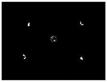 | 32 | 100% |
| Four areas | 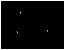 |  | 67 | 100% |
| Three areas |  |  | 54 | 100% |
| Non-opposite two areas |  |  | 65 | 96.9% |
| Opposite areas | 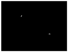 | 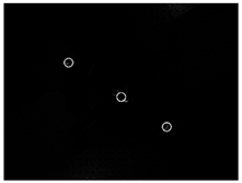 | 44 | 93.18% |
| One area | 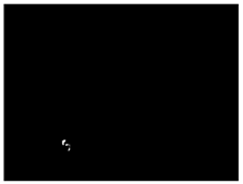 |  | 38 | 86.8% |
Disclaimer/Publisher’s Note: The statements, opinions and data contained in all publications are solely those of the individual author(s) and contributor(s) and not of MDPI and/or the editor(s). MDPI and/or the editor(s) disclaim responsibility for any injury to people or property resulting from any ideas, methods, instructions or products referred to in the content. |
© 2024 by the authors. Licensee MDPI, Basel, Switzerland. This article is an open access article distributed under the terms and conditions of the Creative Commons Attribution (CC BY) license (https://creativecommons.org/licenses/by/4.0/).
Share and Cite
Jiang, B.; Zhang, H.-Y.; Su, W.-H. Automatic Localization of Soybean Seedlings Based on Crop Signaling and Multi-View Imaging. Sensors 2024, 24, 3066. https://doi.org/10.3390/s24103066
Jiang B, Zhang H-Y, Su W-H. Automatic Localization of Soybean Seedlings Based on Crop Signaling and Multi-View Imaging. Sensors. 2024; 24(10):3066. https://doi.org/10.3390/s24103066
Chicago/Turabian StyleJiang, Bo, He-Yi Zhang, and Wen-Hao Su. 2024. "Automatic Localization of Soybean Seedlings Based on Crop Signaling and Multi-View Imaging" Sensors 24, no. 10: 3066. https://doi.org/10.3390/s24103066
APA StyleJiang, B., Zhang, H.-Y., & Su, W.-H. (2024). Automatic Localization of Soybean Seedlings Based on Crop Signaling and Multi-View Imaging. Sensors, 24(10), 3066. https://doi.org/10.3390/s24103066