


Physics-Informed Neural Networks for the Condition Monitoring of Rotating Shafts


Abstract
:1. Introduction
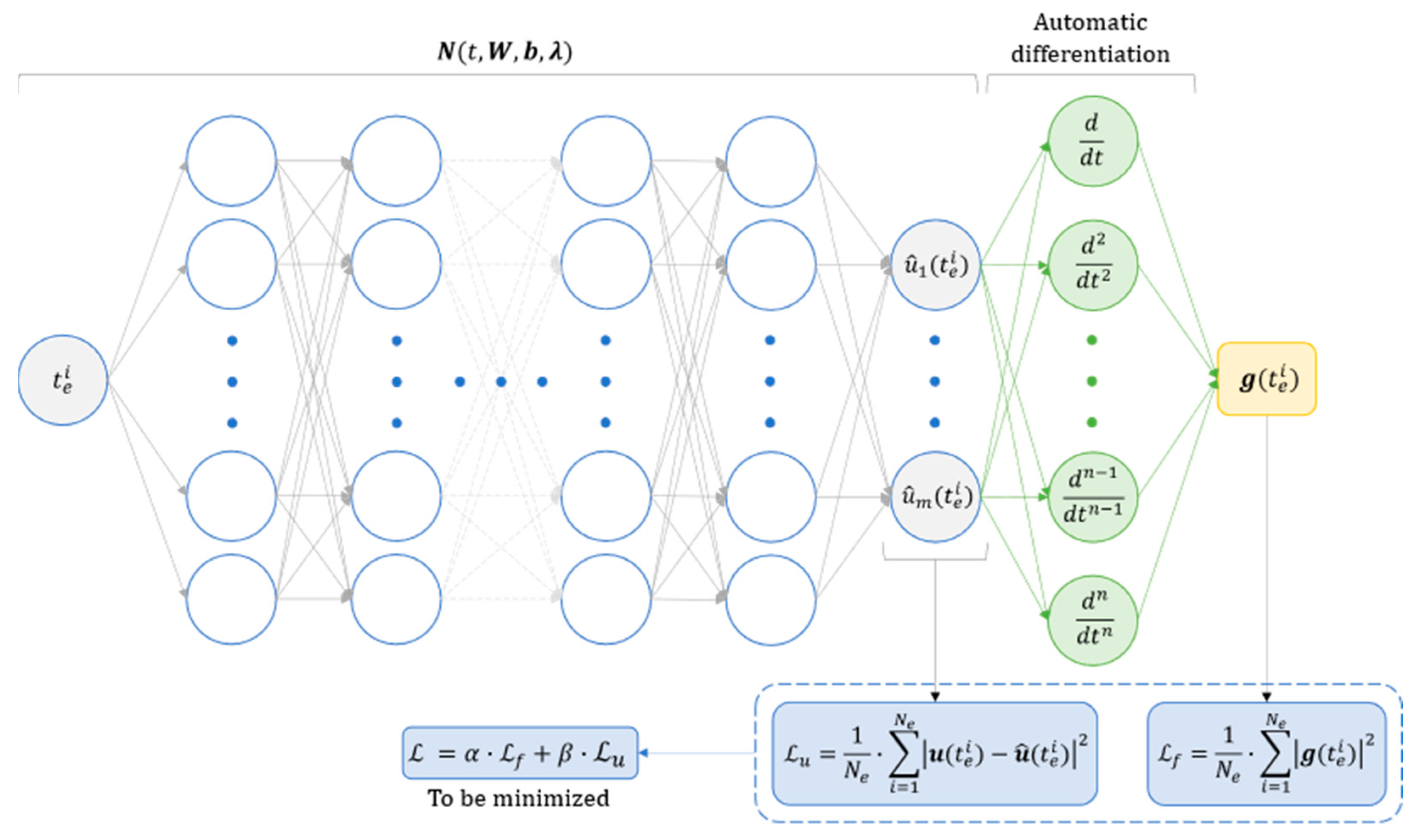
2. Methodology
3. Case Study
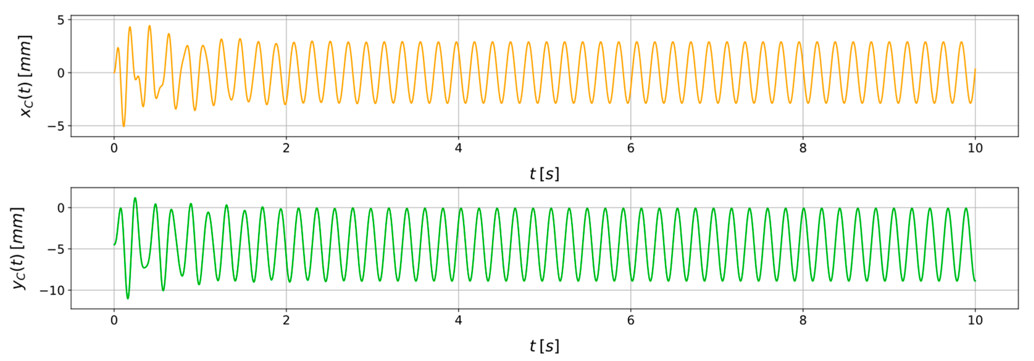
3.1. Extended Jeffcott Rotor with Unknown System Parameters
3.2. System State Characterization through Physics-Informed Neural Networks
3.3. Comparison with Traditional Optimization Algorithms for Parameters Estimation
4. Conclusions
Author Contributions
Funding
Institutional Review Board Statement
Informed Consent Statement
Data Availability Statement
Conflicts of Interest
References
- Tandon, N.; Parey, A. Condition Monitoring of Rotary Machines. In Condition Monitoring and Control for Intelligent Manufacturing; Springer: Berlin/Heidelberg, Germany, 2006; pp. 109–136. [Google Scholar] [CrossRef]
- Jeong, H.; Park, S.; Woo, S.; Lee, S. Rotating Machinery Diagnostics Using Deep Learning on Orbit Plot Images. Procedia Manuf. 2016, 5, 1107–1118. [Google Scholar] [CrossRef]
- Tiboni, M.; Remino, C.; Bussola, R.; Amici, C. A Review on Vibration-Based Condition Monitoring of Rotating Machinery. Appl. Sci. 2022, 12, 972. [Google Scholar] [CrossRef]
- Silva, D.; Mendes, J.C.; Pereira, A.B.; Gégot, F.; Alves, L.N. Measuring Torque and Temperature in a Rotating Shaft Using Commercial SAW Sensors. Sensors 2017, 17, 1547. [Google Scholar] [CrossRef] [PubMed]
- Nandi, S.; Toliyat, H.A.; Li, X. Condition Monitoring and Fault Diagnosis of Electrical Motors—A Review. IEEE Trans. Energy Convers. 2005, 20, 719–729. [Google Scholar] [CrossRef]
- Farrar, C.R.; Worden, K. An Introduction to Structural Health Monitoring. Philos. Trans. R. Soc. A Math. Phys. Eng. Sci. 2006, 365, 303–315. [Google Scholar] [CrossRef] [PubMed]
- Hameed, Z.; Hong, Y.S.; Cho, Y.M.; Ahn, S.H.; Song, C.K. Condition Monitoring and Fault Detection of Wind Turbines and Related Algorithms: A Review. Renew. Sustain. Energy Rev. 2009, 13, 1–39. [Google Scholar] [CrossRef]
- Zhou, H.; Huang, X.; Wen, G.; Lei, Z.; Dong, S.; Zhang, P.; Chen, X. Construction of Health Indicators for Condition Monitoring of Rotating Machinery: A Review of the Research. Expert Syst. Appl. 2022, 203, 117297. [Google Scholar] [CrossRef]
- Bogue, R. Sensors for Condition Monitoring: A Review of Technologies and Applications. Sens. Rev. 2013, 33, 295–299. [Google Scholar] [CrossRef]
- Sohn, H. Effects of Environmental and Operational Variability on Structural Health Monitoring. Philos. Trans. R. Soc. A Math. Phys. Eng. Sci. 2006, 365, 539–560. [Google Scholar] [CrossRef]
- Parziale, M.; Lomazzi, L.; Giglio, M.; Cadini, F. Vibration-Based Structural Health Monitoring Exploiting a Combination of Convolutional Neural Networks and Autoencoders for Temperature Effects Neutralization. Struct. Control Health Monit. 2022, 29, e3076. [Google Scholar] [CrossRef]
- Zhao, R.; Yan, R.; Chen, Z.; Mao, K.; Wang, P.; Gao, R.X. Deep Learning and Its Applications to Machine Health Monitoring. Mech. Syst. Signal Process. 2019, 115, 213–237. [Google Scholar] [CrossRef]
- Fu, J.; Chu, J.; Guo, P.; Chen, Z. Condition Monitoring of Wind Turbine Gearbox Bearing Based on Deep Learning Model. IEEE Access 2019, 7, 57078–57087. [Google Scholar] [CrossRef]
- O’Shea, K.; Nash, R. An Introduction to Convolutional Neural Networks. Int. J. Res. Appl. Sci. Eng. Technol. 2015, 10, 943–947. [Google Scholar] [CrossRef]
- Schmidt, R.M. Recurrent Neural Networks (RNNs): A Gentle Introduction and Overview. arXiv 2019, arXiv:1912.05911. [Google Scholar]
- Souza, R.M.; Nascimento, E.G.S.; Miranda, U.A.; Silva, W.J.D.; Lepikson, H.A. Deep Learning for Diagnosis and Classification of Faults in Industrial Rotating Machinery. Comput. Ind. Eng. 2021, 153, 107060. [Google Scholar] [CrossRef]
- Wisal, M.; Oh, K.Y. A New Deep Learning Framework for Imbalance Detection of a Rotating Shaft. Sensors 2023, 23, 7141. [Google Scholar] [CrossRef] [PubMed]
- He, K.; Zhang, X.; Ren, S.; Sun, J. Deep Residual Learning for Image Recognition. In Proceedings of the EEE Conference on Computer Vision and Pattern Recognition, Las Vegas, NV, USA, 27–30 June 2016; pp. 770–778. [Google Scholar]
- Chen, Y.; Rao, M.; Feng, K.; Niu, G. Modified Varying Index Coefficient Autoregression Model for Representation of the Nonstationary Vibration from a Planetary Gearbox. IEEE Trans. Instrum. Meas. 2023, 72, 3511812. [Google Scholar] [CrossRef]
- Han, T.; Xie, W.; Pei, Z. Semi-Supervised Adversarial Discriminative Learning Approach for Intelligent Fault Diagnosis of Wind Turbine. Inf. Sci. 2023, 648, 119496. [Google Scholar] [CrossRef]
- Dosilovic, F.K.; Brcic, M.; Hlupic, N. Explainable Artificial Intelligence: A Survey. In Proceedings of the 2018 41st International Convention on Information and Communication Technology, Electronics and Microelectronics (MIPRO), Opatija, Croatia, 21–25 May 2018; pp. 210–215. [Google Scholar] [CrossRef]
- Lomazzi, L.; Fabiano, S.; Parziale, M.; Giglio, M.; Cadini, F. On the Explainability of Convolutional Neural Networks Processing Ultrasonic Guided Waves for Damage Diagnosis. Mech. Syst. Signal Process. 2023, 183, 109642. [Google Scholar] [CrossRef]
- Parziale, M.; Lomazzi, L.; Giglio, M.; Cadini, F. Transmissibility Functions-Based Structural Damage Assessment with the Use of Explainable Convolutional Neural Networks. In International Conference on Experimental Vibration Analysis for Civil Engineering Structures; Springer Nature: Cham, Switzerland, 2023; pp. 540–549. [Google Scholar] [CrossRef]
- Parziale, M.; Henrique Silva, P.; Giglio, M.; Cadini, F. Explainability of Convolutional Neural Networks for Damage Diagnosis Using Transmissibility Functions. Available online: http://dx.doi.org/10.2139/ssrn.4545333 (accessed on 27 December 2023).
- Parziale, M.; Yeung, Y.F.; Youcef-Toumi, K.; Giglio, M.; Cadini, F. Anomaly Characterization for the Condition Monitoring of Rotating Shafts Exploiting Data Fusion and Explainable Convolutional Neural Networks. Available online: http://dx.doi.org/10.2139/ssrn.4634978 (accessed on 27 December 2023).
- Raissi, M.; Perdikaris, P.; Karniadakis, G.E. Physics-Informed Neural Networks: A Deep Learning Framework for Solving Forward and Inverse Problems Involving Nonlinear Partial Differential Equations. J. Comput. Phys. 2019, 378, 686–707. [Google Scholar] [CrossRef]
- Raissi, M.; Perdikaris, P.; Karniadakis, G.E. Physics Informed Deep Learning (Part I): Data-Driven Solutions of Nonlinear Partial Differential Equations. arXiv 2017, arXiv:1711.10561. [Google Scholar]
- Haghighat, E.; Raissi, M.; Moure, A.; Gomez, H.; Juanes, R. A Physics-Informed Deep Learning Framework for Inversion and Surrogate Modeling in Solid Mechanics. Comput. Methods Appl. Mech. Eng. 2021, 379, 113741. [Google Scholar] [CrossRef]
- Chen, Y.; Rao, M.; Feng, K.; Zuo, M.J. Physics-Informed LSTM Hyperparameters Selection for Gearbox Fault Detection. Mech. Syst. Signal Process. 2022, 171, 108907. [Google Scholar] [CrossRef]
- Shen, S.; Lu, H.; Sadoughi, M.; Hu, C.; Nemani, V.; Thelen, A.; Webster, K.; Darr, M.; Sidon, J.; Kenny, S. A Physics-Informed Deep Learning Approach for Bearing Fault Detection. Eng. Appl. Artif. Intell. 2021, 103, 104295. [Google Scholar] [CrossRef]
- Garpelli, L.N.; Alves, D.S.; Cavalca, K.L.; de Castro, H.F. Physics-Guided Neural Networks Applied in Rotor Unbalance Problems. Struct. Health Monit. 2023, 22, 4117–4130. [Google Scholar] [CrossRef]
- Deng, W.; Nguyen, K.T.P.; Medjaher, K.; Gogu, C.; Morio, J. Rotor Dynamics Informed Deep Learning for Detection, Identification, and Localization of Shaft Crack and Unbalance Defects. Adv. Eng. Inform. 2023, 58, 102128. [Google Scholar] [CrossRef]
- Cybenko, G. Approximation by Superpositions of a Sigmoidal Function. Math. Control. Signals Syst. 1989, 2, 303–314. [Google Scholar] [CrossRef]
- Wang, S.-C. Artificial Neural Network. In Interdisciplinary Computing in Java Programming; Springer: Berlin/Heidelberg, Germany, 2003; pp. 81–100. [Google Scholar] [CrossRef]
- Margossian, C.C.; Charles Margossian, C.C. A Review of Automatic Differentiation and Its Efficient Implementation. Wiley Interdiscip. Rev. Data Min. Knowl. Discov. 2019, 9, e1305. [Google Scholar] [CrossRef]
- Al Seyab, R.K.; Cao, Y. Nonlinear System Identification for Predictive Control Using Continuous Time Recurrent Neural Networks and Automatic Differentiation. J. Process Control 2008, 18, 568–581. [Google Scholar] [CrossRef]
- Genta, G.; Keith, R.H. Vibration Dynamics and Control. Noise Control Eng. J. 2009, 57, 156. [Google Scholar] [CrossRef]
- Cerrada, M.; Sánchez, R.V.; Li, C.; Pacheco, F.; Cabrera, D.; Valente de Oliveira, J.; Vásquez, R.E. A Review on Data-Driven Fault Severity Assessment in Rolling Bearings. Mech. Syst. Signal Process. 2018, 99, 169–196. [Google Scholar] [CrossRef]
- Bogacki, P.; Shampine, L.F. An Efficient Runge-Kutta (4,5) Pair. Comput. Math. Appl. 1996, 32, 15–28. [Google Scholar] [CrossRef]
- Rumelhart, D.E.; Hinton, G.E.; Williams, R.J. Learning Representations by Back-Propagating Errors. Nature 1986, 323, 533–536. [Google Scholar] [CrossRef]
- Liu, D.C.; Nocedal, J. On the Limited Memory BFGS Method for Large Scale Optimization. Math. Program. 1989, 45, 503–528. [Google Scholar] [CrossRef]
- Bengio, Y. Gradient-Based Optimization of Hyperparameters. Neural Comput. 2000, 12, 1889–1900. [Google Scholar] [CrossRef]
- Elsayed, S.M.; Sarker, R.A.; Essam, D.L. A New Genetic Algorithm for Solving Optimization Problems. Eng. Appl. Artif. Intell. 2014, 27, 57–69. [Google Scholar] [CrossRef]


| Unknown Parameter | True Value | PINN Estimation | Relative Error (%) |
|---|---|---|---|
| [mm] | |||
| [deg] | |||
| [N·s·mm−1] | |||
| [N·mm−1] | |||
| [N·mm−1] |
| Unknown Parameter | True Value | PINN Estimation | Relative Error (%) |
|---|---|---|---|
| [mm] | |||
| [deg] | |||
| [N·s·mm−1] | |||
| [N·mm−1] | |||
| [N·mm−1] |
| Unknown Parameter | True Value | PINN Estimation | Relative Error (%) |
|---|---|---|---|
| [mm] | |||
| [deg] | |||
| [N·s·mm−1] | |||
| [N·mm−1] | |||
| [N·mm−1] |
| Unknown Parameter | True Value | Gradient-Based Method | Genetic Algorithm | ||
|---|---|---|---|---|---|
| Estimation | Relative Error (%) | Estimation | Relative Error (%) | ||
| [mm] | 0.00 | 7.60 | 5.00 | ||
| [deg] | 99.80 | 20.53 | 105.30 | ||
| [N·s·mm−1] | 13.00 | 0.86 | |||
| [N·mm−1] | 2.35 | 5.39 | 2.53 | ||
| [N·mm−1] | 1.52 | 7.25 | 0.00 | ||
| Unknown Parameter | True Value | Gradient-Based Method | Genetic Algorithm | ||
|---|---|---|---|---|---|
| Estimation | Relative Error (%) | Estimation | Relative Error (%) | ||
| [mm] | 7.99 | 0.12 | 7.40 | 7.50 | |
| [deg] | 99.90 | 1.92 | 80.80 | ||
| [N·s·mm−1] | 13.00 | 30.86 | |||
| [N·mm−1] | 2.35 | 5.66 | 2.35 | ||
| [N·mm−1] | 1.38 | 7.30 | 0.69 | ||
| Unknown Parameter | True Value | Gradient-Based Method | Genetic Algorithm | ||
|---|---|---|---|---|---|
| Estimation | Relative Error (%) | Estimation | Relative Error (%) | ||
| [mm] | 1.67 | 10.2 | 15.00 | ||
| [deg] | 2.20 | 19.8 | 1.00 | ||
| [N·s·mm−1] | 8.20 | 0.40 | |||
| [N·mm−1] | 0.00 | 7.53 | 2.96 | ||
| [N·mm−1] | 0.65 | 6.12 | 0.33 | ||
Disclaimer/Publisher’s Note: The statements, opinions and data contained in all publications are solely those of the individual author(s) and contributor(s) and not of MDPI and/or the editor(s). MDPI and/or the editor(s) disclaim responsibility for any injury to people or property resulting from any ideas, methods, instructions or products referred to in the content. |
© 2023 by the authors. Licensee MDPI, Basel, Switzerland. This article is an open access article distributed under the terms and conditions of the Creative Commons Attribution (CC BY) license (https://creativecommons.org/licenses/by/4.0/).
Share and Cite
Parziale, M.; Lomazzi, L.; Giglio, M.; Cadini, F. Physics-Informed Neural Networks for the Condition Monitoring of Rotating Shafts. Sensors 2024, 24, 207. https://doi.org/10.3390/s24010207
Parziale M, Lomazzi L, Giglio M, Cadini F. Physics-Informed Neural Networks for the Condition Monitoring of Rotating Shafts. Sensors. 2024; 24(1):207. https://doi.org/10.3390/s24010207
Chicago/Turabian StyleParziale, Marc, Luca Lomazzi, Marco Giglio, and Francesco Cadini. 2024. "Physics-Informed Neural Networks for the Condition Monitoring of Rotating Shafts" Sensors 24, no. 1: 207. https://doi.org/10.3390/s24010207
APA StyleParziale, M., Lomazzi, L., Giglio, M., & Cadini, F. (2024). Physics-Informed Neural Networks for the Condition Monitoring of Rotating Shafts. Sensors, 24(1), 207. https://doi.org/10.3390/s24010207