Investigation on the Impact of Excitation Amplitude on AFM-TM Microcantilever Beam System’s Dynamic Characteristics and Implementation of an Equivalent Circuit


Abstract
:1. Introduction
2. Mathematical Model
2.1. Mathematical Model of System 1
2.2. Mathematical Model of System 2
3. The Influence of Excitation Amplitude on the Movement Properties of System 2 and System 1
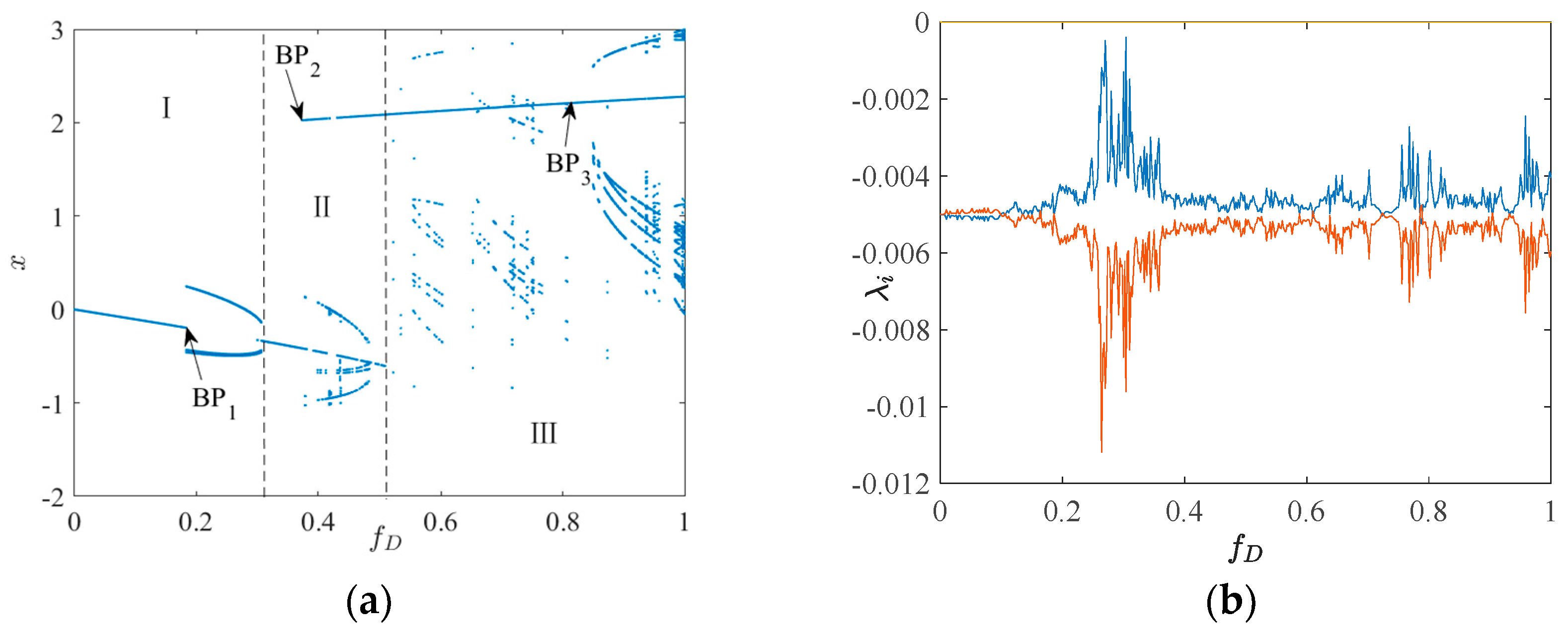
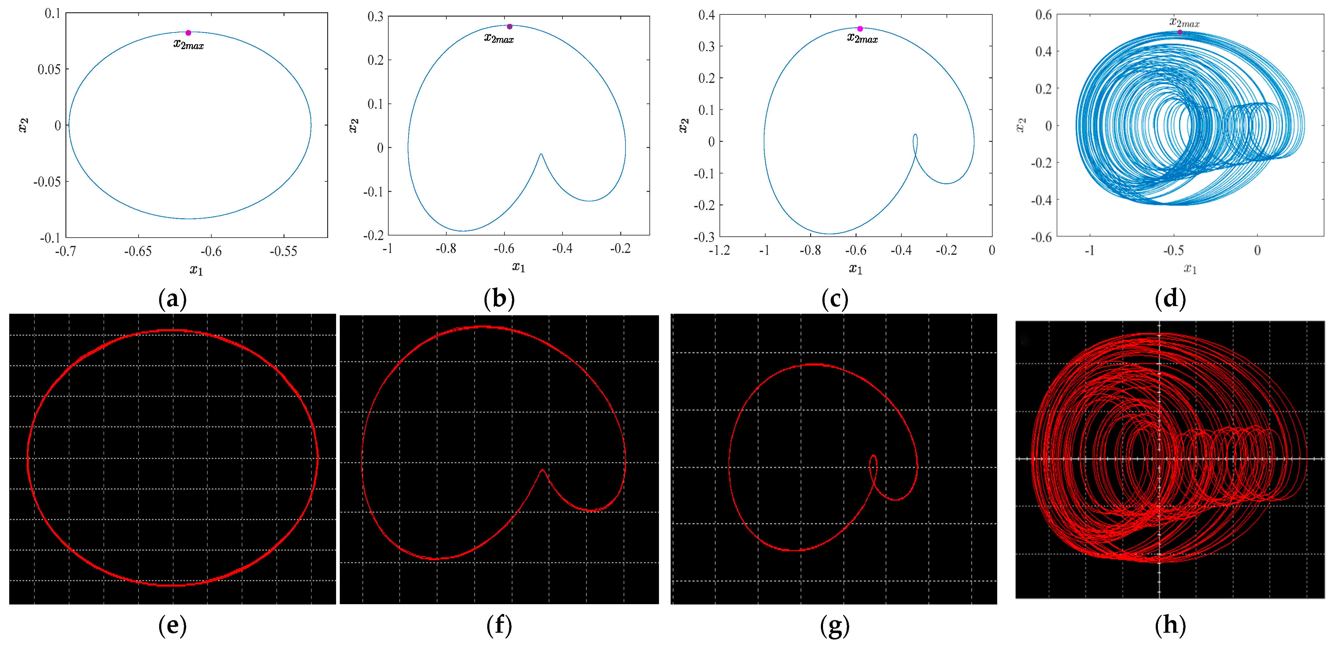
3.1. System 2
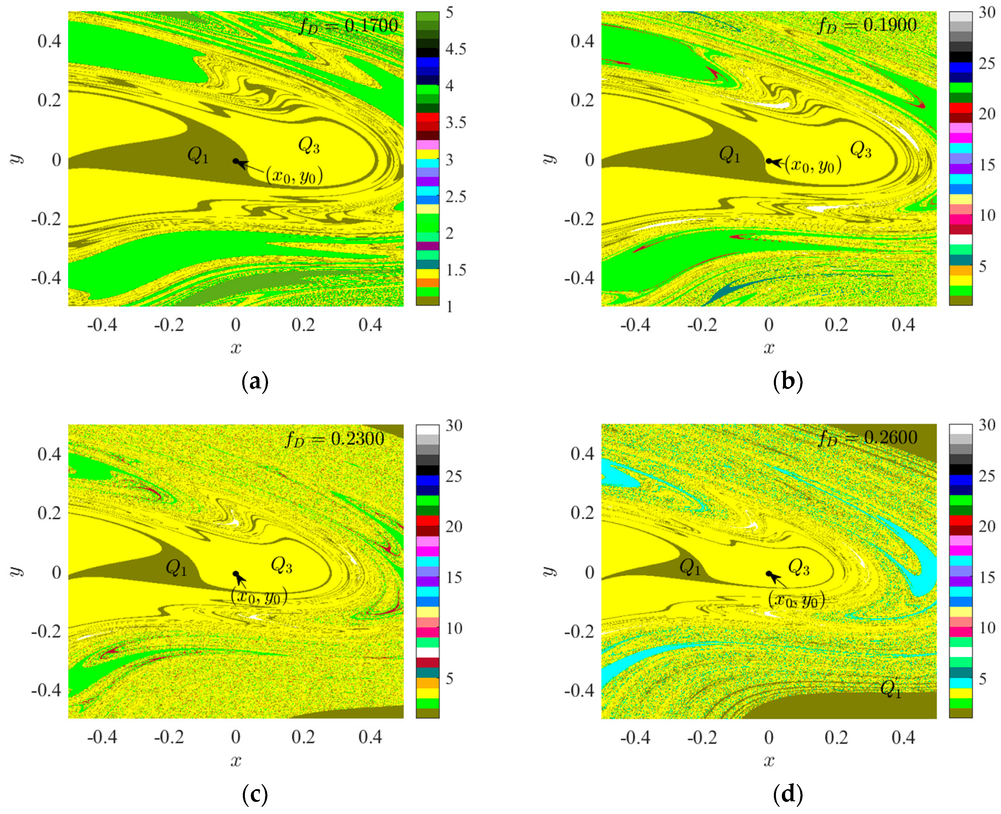
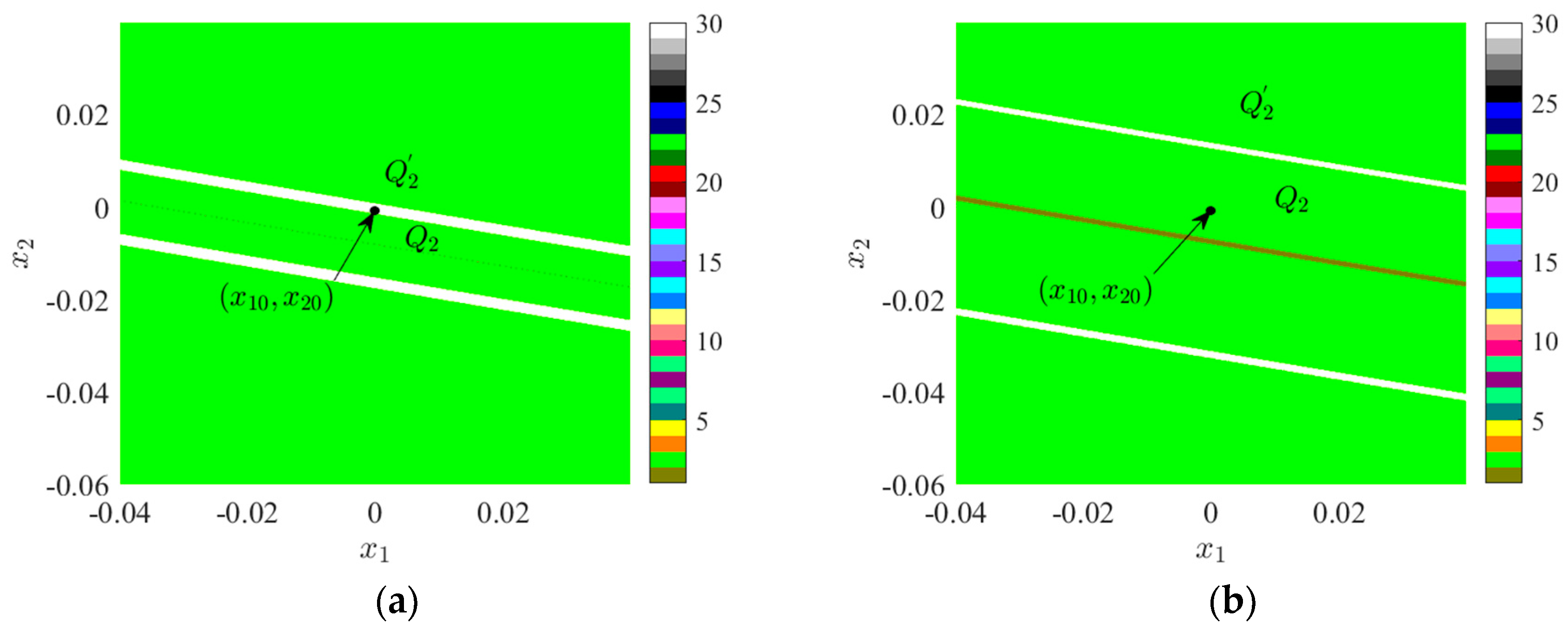
3.1.1. I—Regional Suction Basin Analysis
3.1.2. II—Regional Suction Basin Analysis
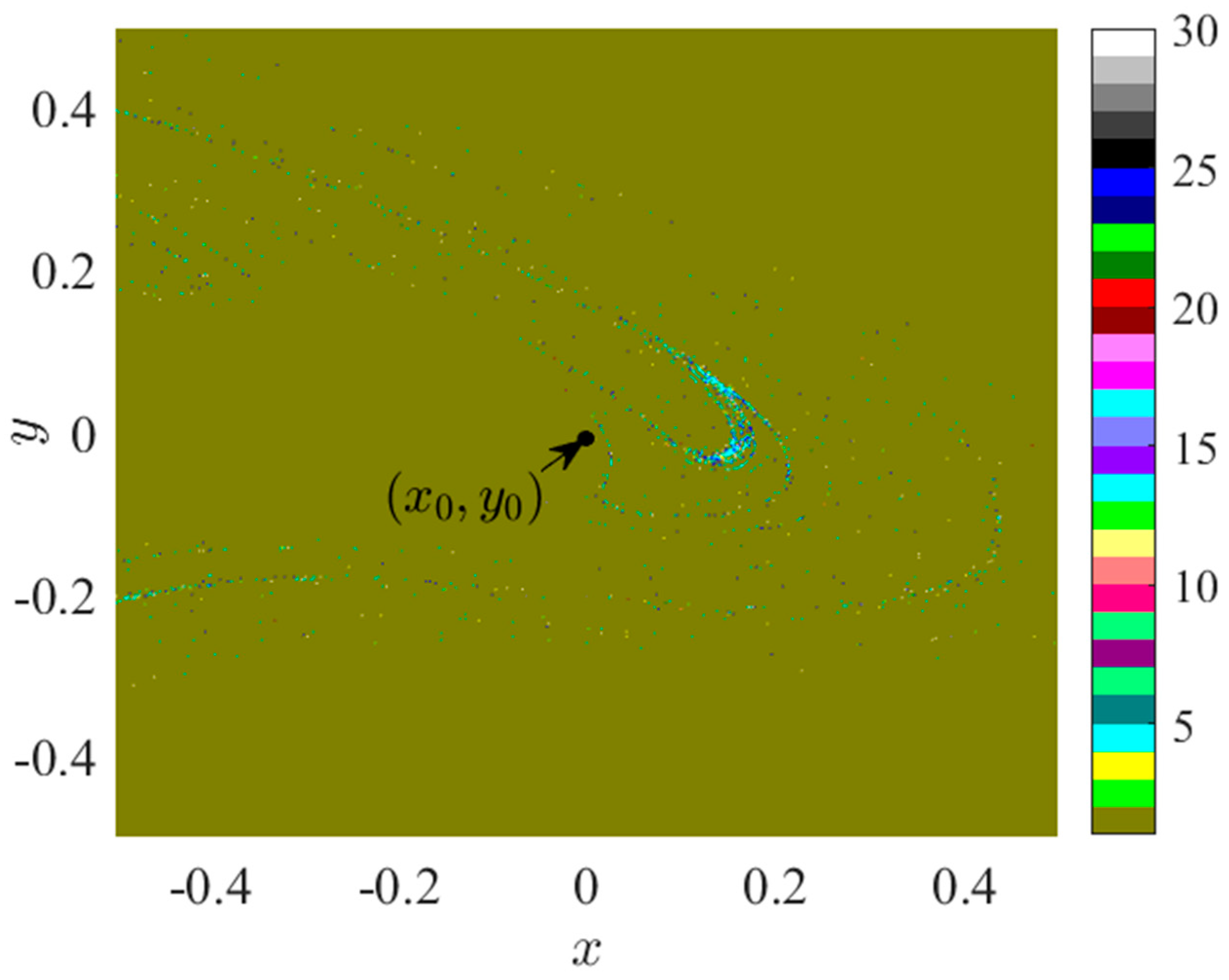
3.1.3. III—Regional Suction Basin Analysis
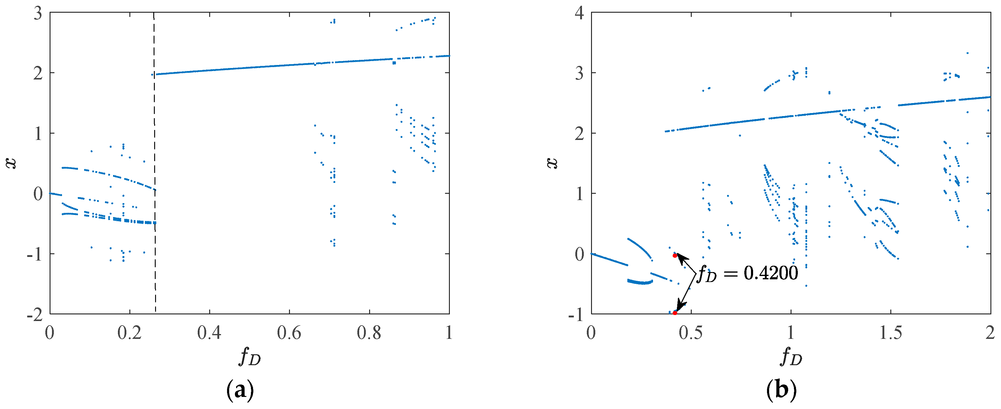
3.2. System 1
4. Simulation of an Equivalent Circuit for the AFM-TM Microcantilever Beam System
4.1. Equivalent Circuit Design
4.2. Simulation of AFM-TM Equivalent Circuit Using Software
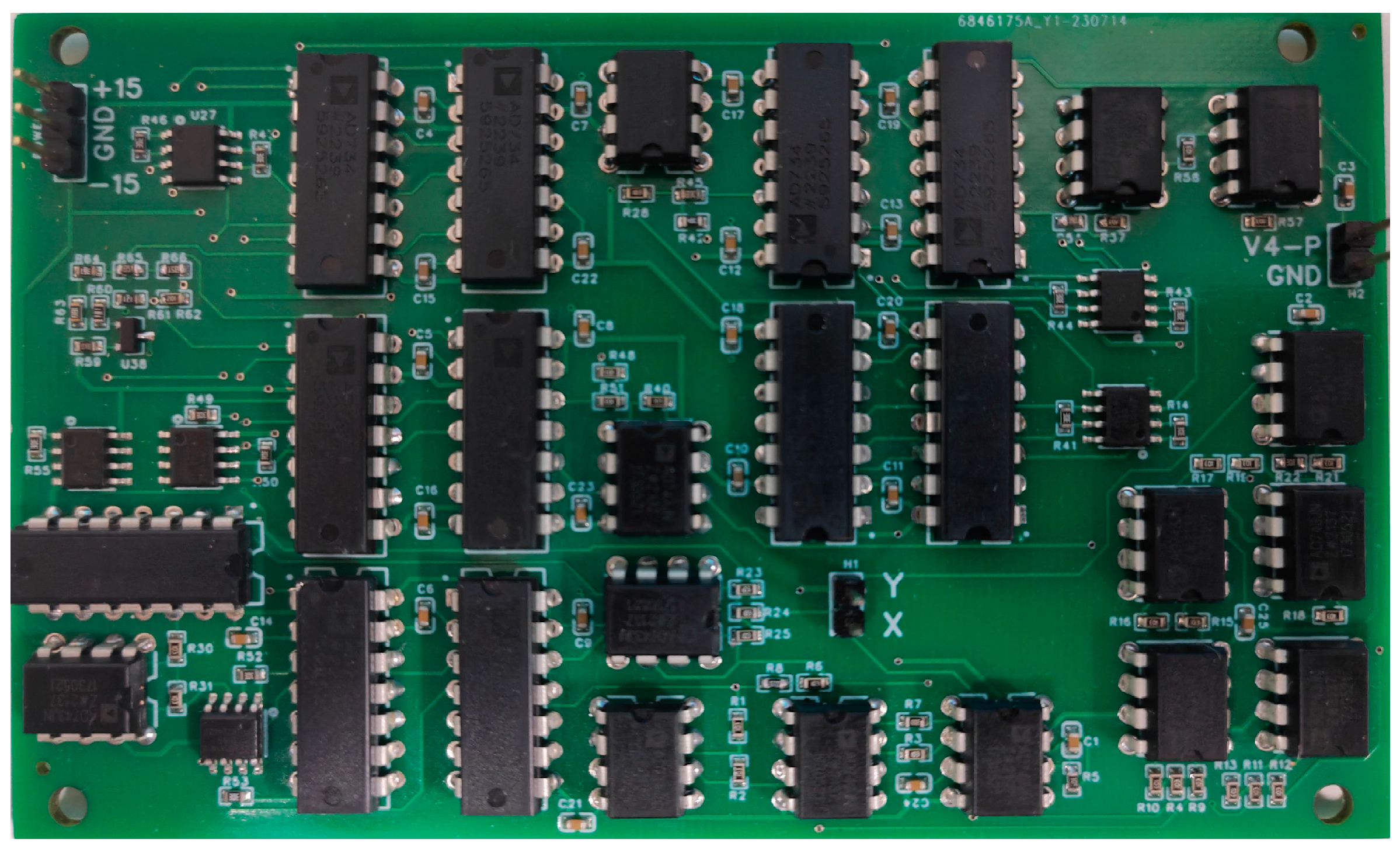
4.3. PCB Simulation Experiment
5. Discussion and Conclusions
Author Contributions
Funding
Institutional Review Board Statement
Informed Consent Statement
Data Availability Statement
Acknowledgments
Conflicts of Interest
References
- Qiu, F.; Song, H.; Feng, W.; Yang, Z.; Zhang, F.; Hu, X. Molecular Dynamics Simulations of the Interaction Between Graphene and Lubricating Oil Molecules. Tribol. Lett. 2023, 71, 33. [Google Scholar] [CrossRef]
- Jadidi, M.; Moghtadernejad, S.; Hanson, J. Numerical Study of the Effects of Twin-Fluid Atomization on the Suspension Plasma Spraying Process. Fluids 2020, 5, 224. [Google Scholar] [CrossRef]
- Peng, Y.; Zhang, H.; Huang, X.-W.; Huang, J.-H.; Luo, M.-B. Monte Carlo Simulation on the Dynamics of a Semi-Flexible Polymer in the Presence of Nanoparticles. Phys. Chem. Chem. Phys. 2018, 20, 26333–26343. [Google Scholar] [CrossRef] [PubMed]
- Tusset, A.M.; Balthazar, J.M.; Ribeiro, M.A.; Lenz, W.B.; Rocha, R.T. Chaos Control of an Atomic Force Microscopy Model in Fractional-Order. Eur. Phys. J. Spec. Top. 2021, 230, 3643–3654. [Google Scholar] [CrossRef]
- Payam, A.F. Modelling and Nanoscale Force Spectroscopy of Frequency Modulation Atomic Force Microscopy. Appl. Math. Model. 2020, 79, 544–554. [Google Scholar] [CrossRef]
- Ito, S.; Schitter, G. Atomic Force Microscopy Capable of Vibration Isolation with Low-Stiffness Z-Axis Actuation. Ultramicroscopy 2018, 186, 9–17. [Google Scholar] [CrossRef]
- Giessibl, F.J. The qPlus Sensor, a Powerful Core for the Atomic Force Microscope. Rev. Sci. Instrum. 2019, 90, 011101. [Google Scholar] [CrossRef] [PubMed]
- Xing, C.; Jiang, W.; Li, M.; Wang, M.; Xiao, J.; Xu, Z. Application of Atomic Force Microscopy in Bitumen Materials at the Nanoscale: A Review. Constr. Build. Mater. 2022, 342, 128059. [Google Scholar] [CrossRef]
- Kitamura, M.; Umemura, K. Hybridization of Papain Molecules and DNA-Wrapped Single-Walled Carbon Nanotubes Evaluated by Atomic Force Microscopy in Fluids. Sci. Rep. 2023, 13, 4833. [Google Scholar] [CrossRef]
- Stan, G.; King, S.W. Atomic Force Microscopy for Nanoscale Mechanical Property Characterization. J. Vac. Sci. Technol. B Nanotechnol. Microelectron. Mater. Process. Meas. Phenom. 2020, 38, 060801. [Google Scholar] [CrossRef]
- Von Eysmondt, H.; Schäffer, T.E. Scanning Ion Conductance Microscopy and Atomic Force Microscopy: A Comparison of Strengths and Limitations for Biological Investigations. In Scanning Ion Conductance Microscopy; Schäffer, T.E., Ed.; Bioanalytical Reviews; Springer International Publishing: Cham, Switzerland, 2022; Volume 3, pp. 23–71. ISBN 978-3-031-14442-4. [Google Scholar]
- Krieg, M.; Fläschner, G.; Alsteens, D.; Gaub, B.M.; Roos, W.H.; Wuite, G.J.L.; Gaub, H.E.; Gerber, C.; Dufrêne, Y.F.; Müller, D.J. Atomic Force Microscopy-Based Mechanobiology. Nat. Rev. Phys. 2018, 1, 41–57. [Google Scholar] [CrossRef]
- Müller, D.J.; Dumitru, A.C.; Lo Giudice, C.; Gaub, H.E.; Hinterdorfer, P.; Hummer, G.; De Yoreo, J.J.; Dufrêne, Y.F.; Alsteens, D. Atomic Force Microscopy-Based Force Spectroscopy and Multiparametric Imaging of Biomolecular and Cellular Systems. Chem. Rev. 2021, 121, 11701–11725. [Google Scholar] [CrossRef] [PubMed]
- Miranda, A.; Gómez-Varela, A.I.; Stylianou, A.; Hirvonen, L.M.; Sánchez, H.; De Beule, P.A.A. How Did Correlative Atomic Force Microscopy and Super-Resolution Microscopy Evolve in the Quest for Unravelling Enigmas in Biology? Nanoscale 2021, 13, 2082–2099. [Google Scholar] [CrossRef] [PubMed]
- Belardinelli, P.; Chandrashekar, A.; Alijani, F.; Lenci, S. Non-Smooth Dynamics of Tapping Mode Atomic Force Microscopy. J. Comput. Nonlinear Dyn. 2023, 18, 081004. [Google Scholar] [CrossRef]
- Ribeiro, M.A.; Balthazar, J.M.; Lenz, W.B.; Rocha, R.T.; Tusset, A.M. Numerical Exploratory Analysis of Dynamics and Control of an Atomic Force Microscopy in Tapping Mode with Fractional Order. Shock. Vib. 2020, 2020, 4048307. [Google Scholar] [CrossRef]
- SoltanRezaee, M.; Bodaghi, M. Nonlinear Dynamic Stability of Piezoelectric Thermoelastic Electromechanical Resonators. Sci. Rep. 2020, 10, 2982. [Google Scholar] [CrossRef]
- Rahmanian, S.; Hosseini-Hashemi, S.; SoltanRezaee, M. Efficient Large Amplitude Primary Resonance in In-Extensional Nanocapacitors: Nonlinear Mean Curvature Component. Sci. Rep. 2019, 9, 20256. [Google Scholar] [CrossRef]
- Masoumi, A.; Amiri, A.; Vesal, R.; Rezazadeh, G. Nonlinear Static Pull-in Instability Analysis of Smart Nano-Switch Considering Flexoelectric and Surface Effects via DQM. Proc. Inst. Mech. Eng. Part C J. Mech. Eng. Sci. 2021, 235, 7821–7835. [Google Scholar] [CrossRef]
- Yaghoobi, M.; Koochi, A. Electromagnetic Instability Analysis of Functionally Graded Tapered Nano-Tweezers. Phys. Scr. 2021, 96, 085701. [Google Scholar] [CrossRef]
- Rahmanian, S.; Hosseini-Hashemi, S. Size-Dependent Resonant Response of a Double-Layered Viscoelastic Nanoresonator under Electrostatic and Piezoelectric Actuations Incorporating Surface Effects and Casimir Regime. Int. J. Non-Linear Mech. 2019, 109, 118–131. [Google Scholar] [CrossRef]
- Xu, Q.; Cheng, S.; Ju, Z.; Chen, M.; Wu, H. Asymmetric Coexisting Bifurcations and Multi-Stability in an Asymmetric Memristive Diode-Bridge-Based Jerk Circuit. Chin. J. Phys. 2021, 70, 69–81. [Google Scholar] [CrossRef]
- Lai, Q.; Nestor, T.; Kengne, J.; Zhao, X.-W. Coexisting Attractors and Circuit Implementation of a New 4D Chaotic System with Two Equilibria. Chaos Solitons Fractals 2018, 107, 92–102. [Google Scholar] [CrossRef]
- Luo, J.; Bao, H.; Chen, M.; Xu, Q.; Bao, B. Inductor-Free Multi-Stable Chua’s Circuit Constructed by Improved PI-Type Memristor Emulator and Active Sallen–Key High-Pass Filter. Eur. Phys. J. Spec. Top. 2019, 228, 1983–1994. [Google Scholar] [CrossRef]
- Hua, M.; Yang, S.; Xu, Q.; Chen, M.; Wu, H.; Bao, B. Forward and Reverse Asymmetric Memristor-Based Jerk Circuits. AEU-Int. J. Electron. Commun. 2020, 123, 153294. [Google Scholar] [CrossRef]
- Bhardwaj, K.; Srivastava, M. Mathematical Formulation and OTA Based Emulator for Three Cross-over Memristor. Int. J. Electron. 2021, 108, 1871–1898. [Google Scholar] [CrossRef]
- SoltanRezaee, M.; Bodaghi, M.; Farrokhabadi, A.; Hedayati, R. Nonlinear Stability Analysis of Piecewise Actuated Piezoelectric Microstructures. Int. J. Mech. Sci. 2019, 160, 200–208. [Google Scholar] [CrossRef]
- Rocha, R.; Medrano-T, R.O. Stability Analysis of the Chua’s Circuit with Generic Odd Nonlinearity. Chaos Solitons Fractals 2023, 176, 114112. [Google Scholar] [CrossRef]
- Pei, H. Analysis and Control of Multiple Attractors in Sprott B System. Chaos Solitons Fractals 2019, 123, 192–200. [Google Scholar] [CrossRef]
- Joshi, M.; Ranjan, A. Current-Controlled Chaotic Chua’s Circuit Using CCCII. In Advances in Communication and Computational Technology; Hura, G.S., Singh, A.K., Siong Hoe, L., Eds.; Lecture Notes in Electrical Engineering; Springer Nature Singapore: Singapore, 2021; Volume 668, pp. 535–545. ISBN 9789811553400. [Google Scholar]
- Marcondes, D.W.C.; Comassetto, G.F.; Pedro, B.G.; Vieira, J.C.C.; Hoff, A.; Prebianca, F.; Manchein, C.; Albuquerque, H.A. Extensive Numerical Study and Circuitry Implementation of the Watt Governor Model. Int. J. Bifurc. Chaos 2017, 27, 1750175. [Google Scholar] [CrossRef]
- Foa Torres, L.E.F.; Roche, S.; Charlier, J.-C. Introduction to Graphene-Based Nanomaterials: From Electronic Structure to Quantum Transport, 2nd ed.; Cambridge University Press: Cambridge, UK, 2020; ISBN 978-1-108-66446-2. [Google Scholar]
- Reimers, J.R.; Tawfik, S.A.; Ford, M.J. Van Der Waals Forces Control Ferroelectric–Antiferroelectric Ordering in CuInP 2 S 6 and CuBiP 2 Se 6 Laminar Materials. Chem. Sci. 2018, 9, 7620–7627. [Google Scholar] [CrossRef]
- Gong, T.; Corrado, M.R.; Mahbub, A.R.; Shelden, C.; Munday, J.N. Recent Progress in Engineering the Casimir Effect—Applications to Nanophotonics, Nanomechanics, and Chemistry. Nanophotonics 2020, 10, 523–536. [Google Scholar] [CrossRef]
- Carbó-Dorca, R. A Naïve HMO Study of the Casimir Effect. J. Math. Chem. 2022, 60, 581–585. [Google Scholar] [CrossRef]
- Bimonte, G.; Emig, T.; Graham, N.; Kardar, M. Something Can Come of Nothing: Surface Approaches to Quantum Fluctuations and the Casimir Force. Annu. Rev. Nucl. Part. Sci. 2022, 72, 93–118. [Google Scholar] [CrossRef]
- Palasantzas, G.; Van Zwol, P.J.; De Hosson, J.T.M. Transition from Casimir to van Der Waals Force between Macroscopic Bodies. Appl. Phys. Lett. 2008, 93, 121912. [Google Scholar] [CrossRef]


| Description | Value |
|---|---|
| Length of the microcantilever beam | 449 μm |
| Width of the microcantilever beam | 46 μm |
| Thickness of the microcantilever beam | 1.7 μm |
| Radius of the tip | 0.15 μm |
| Material density of the microcantilever beam | 2330 kg/m3 |
| Elastic modulus of materials used in microcantilever beams | 176 GPa |
| Equivalent stiffness of system coupling | 9.8 N/m |
| The first-order resonance frequency of the microcantilever beam | 16,059 Hz |
| Quality factor of the microcantilever beam | 100 |
| Hamaker constant (attractive) | 1.3596 × 10−70 J·m6 |
| Hamaker constant (repulsive) | 1.865 × 10⁻¹⁹ J |
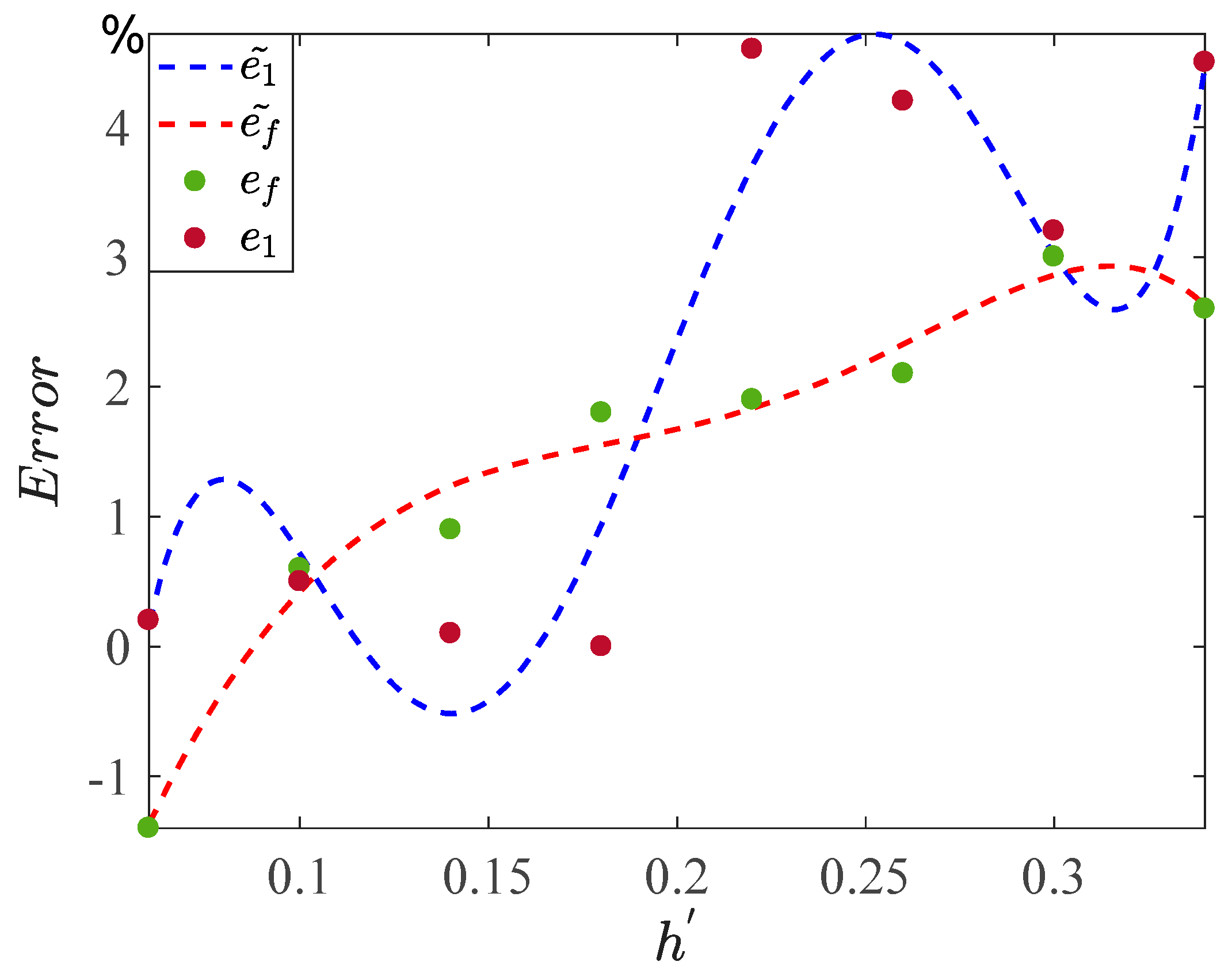
| h’ | y’emax | x2max | f’e | fe | e1 (%) | ef (%) |
|---|---|---|---|---|---|---|
| 0.06 | 0.0833 | 0.0831 | 157 | 159.2 | +0.2 | −1.4 |
| 0.10 | 0.2803 | 0.279 | 160.2 | +0.5 | +0.6 | |
| 0.14 | 0.3580 | 0.3576 | 160.7 | +0.1 | +0.9 | |
| 0.18 | 0.4202 | 0.4204 | 162.1 | 0.0 | +1.8 | |
| 0.22 | 0.5302 | 0.5067 | 162.2 | +4.6 | +1.9 | |
| 0.26 | 0.5966 | 0.5726 | 162.6 | +4.2 | +2.1 | |
| 0.30 | 0.6605 | 0.6398 | 163.9 | +3.2 | +3.0 | |
| 0.34 | 0.7102 | 0.6799 | 163.3 | +4.5 | +2.6 |
Disclaimer/Publisher’s Note: The statements, opinions and data contained in all publications are solely those of the individual author(s) and contributor(s) and not of MDPI and/or the editor(s). MDPI and/or the editor(s) disclaim responsibility for any injury to people or property resulting from any ideas, methods, instructions or products referred to in the content. |
© 2023 by the authors. Licensee MDPI, Basel, Switzerland. This article is an open access article distributed under the terms and conditions of the Creative Commons Attribution (CC BY) license (https://creativecommons.org/licenses/by/4.0/).
Share and Cite
Song, P.; Li, X.; Cui, J.; Chen, K.; Chu, Y. Investigation on the Impact of Excitation Amplitude on AFM-TM Microcantilever Beam System’s Dynamic Characteristics and Implementation of an Equivalent Circuit. Sensors 2024, 24, 107. https://doi.org/10.3390/s24010107
Song P, Li X, Cui J, Chen K, Chu Y. Investigation on the Impact of Excitation Amplitude on AFM-TM Microcantilever Beam System’s Dynamic Characteristics and Implementation of an Equivalent Circuit. Sensors. 2024; 24(1):107. https://doi.org/10.3390/s24010107
Chicago/Turabian StyleSong, Peijie, Xiaojuan Li, Jianjun Cui, Kai Chen, and Yandong Chu. 2024. "Investigation on the Impact of Excitation Amplitude on AFM-TM Microcantilever Beam System’s Dynamic Characteristics and Implementation of an Equivalent Circuit" Sensors 24, no. 1: 107. https://doi.org/10.3390/s24010107
APA StyleSong, P., Li, X., Cui, J., Chen, K., & Chu, Y. (2024). Investigation on the Impact of Excitation Amplitude on AFM-TM Microcantilever Beam System’s Dynamic Characteristics and Implementation of an Equivalent Circuit. Sensors, 24(1), 107. https://doi.org/10.3390/s24010107