
Boosted Convolutional Neural Network Algorithm for the Classification of the Bearing Fault form 1-D Raw Sensor Data


Abstract
1. Introduction
2. Related Works
3. Methodology
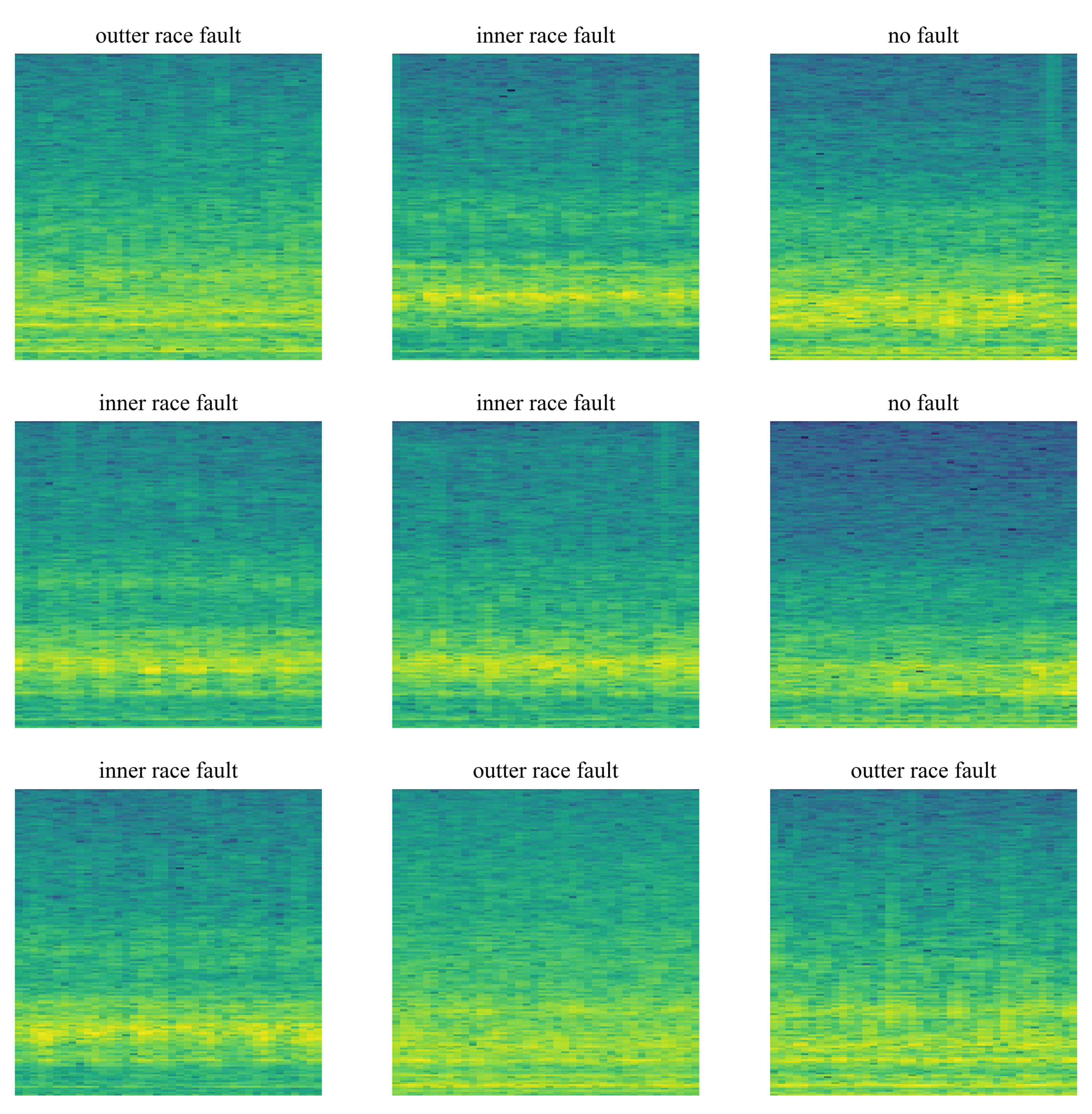
3.1. Spectrogram Model
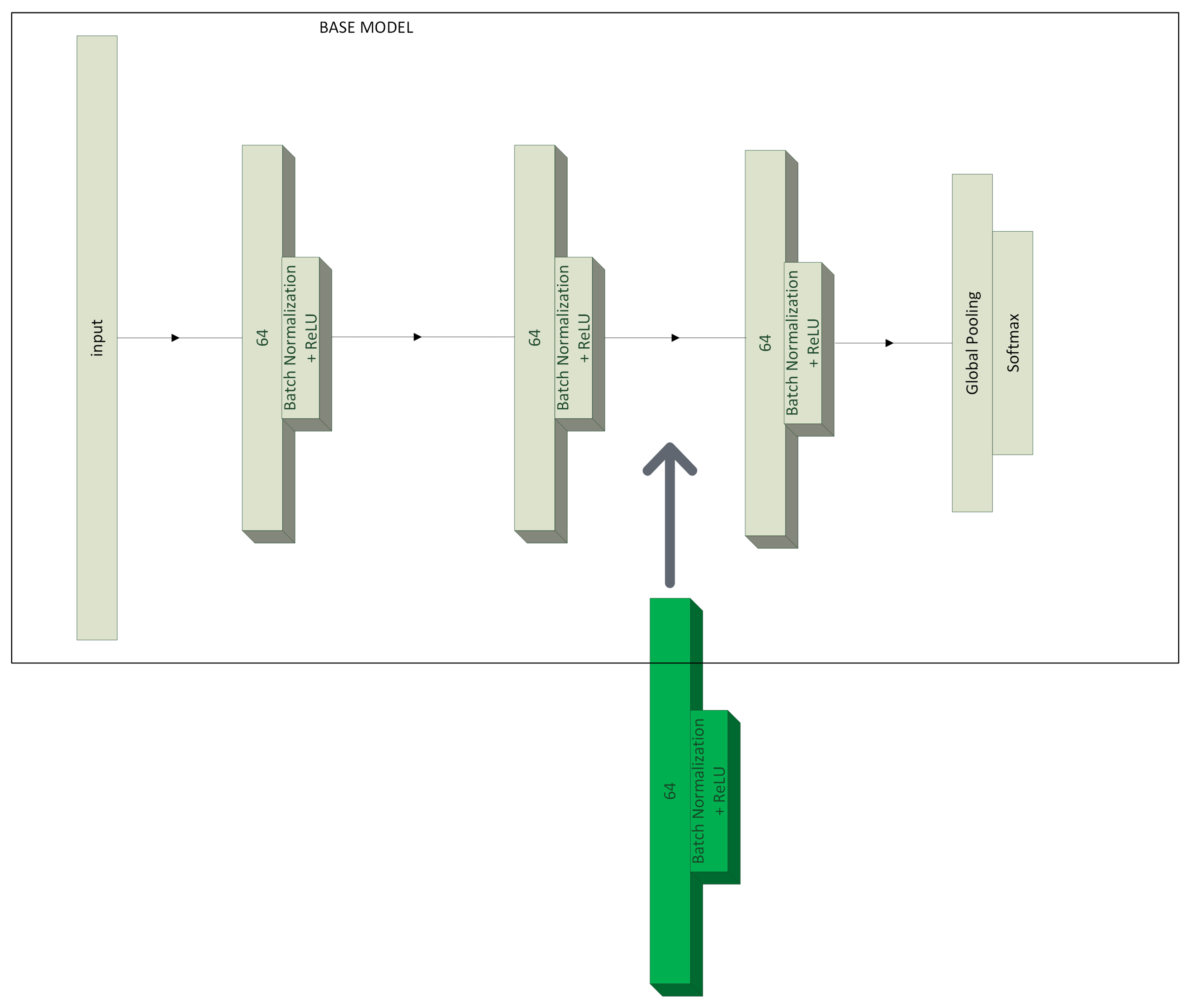
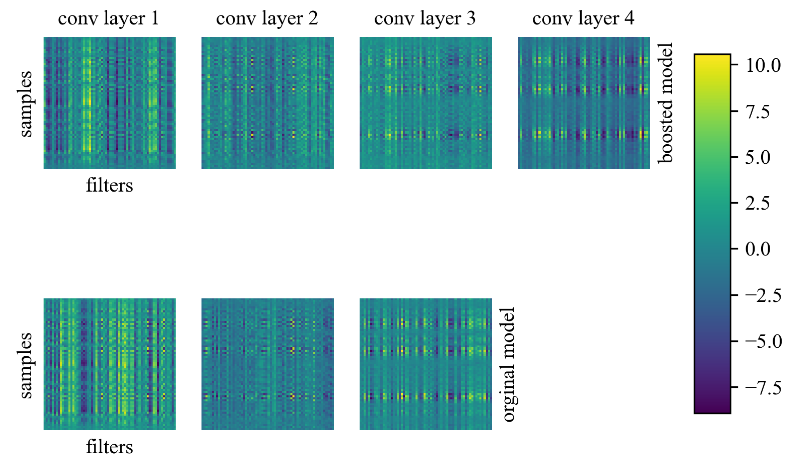
3.2. Time Series Model
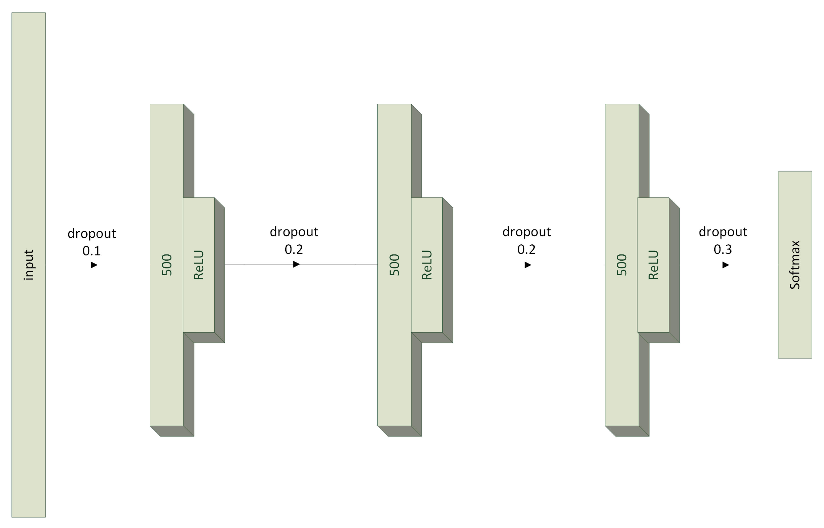
3.3. Multilayer Perceptron Model
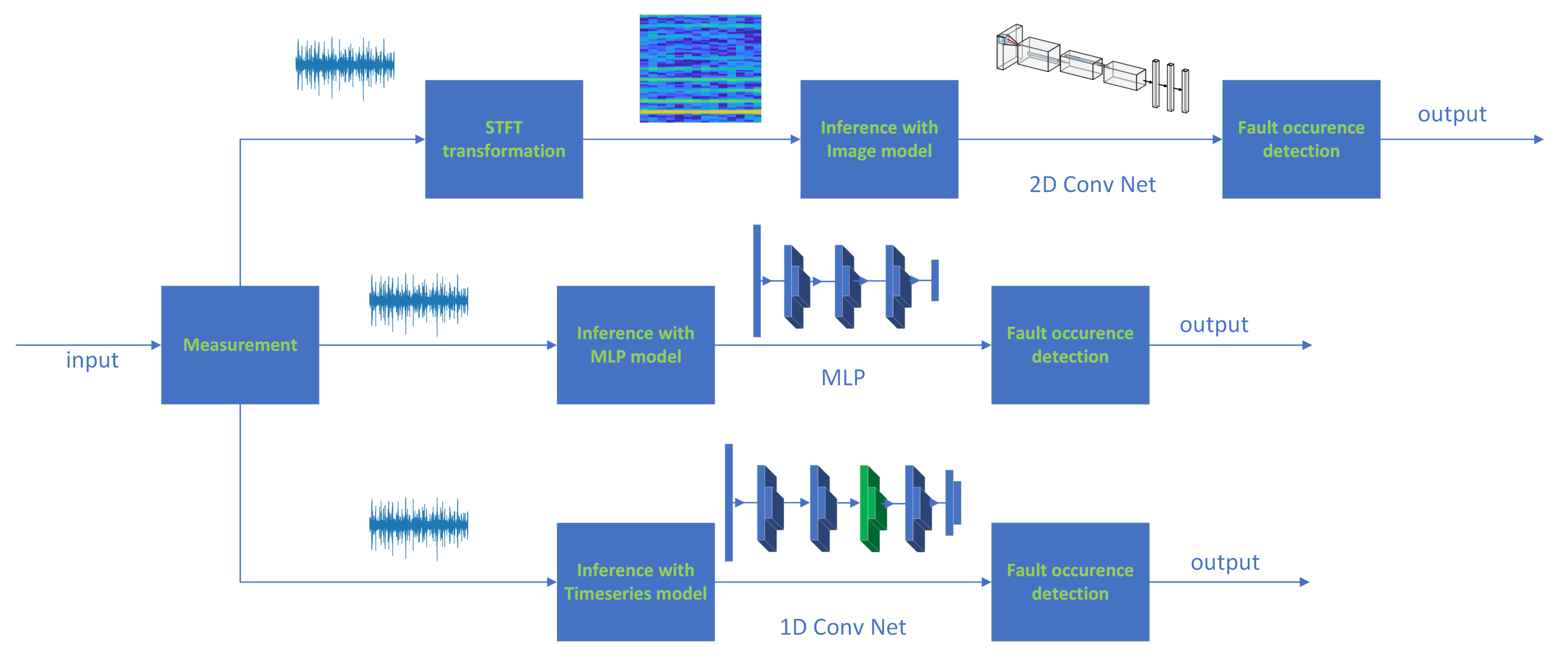
3.4. Method Framework
3.4.1. Framework for MLP and 1D CNN Time Series Models
3.4.2. Framework for the Spectrogram Model
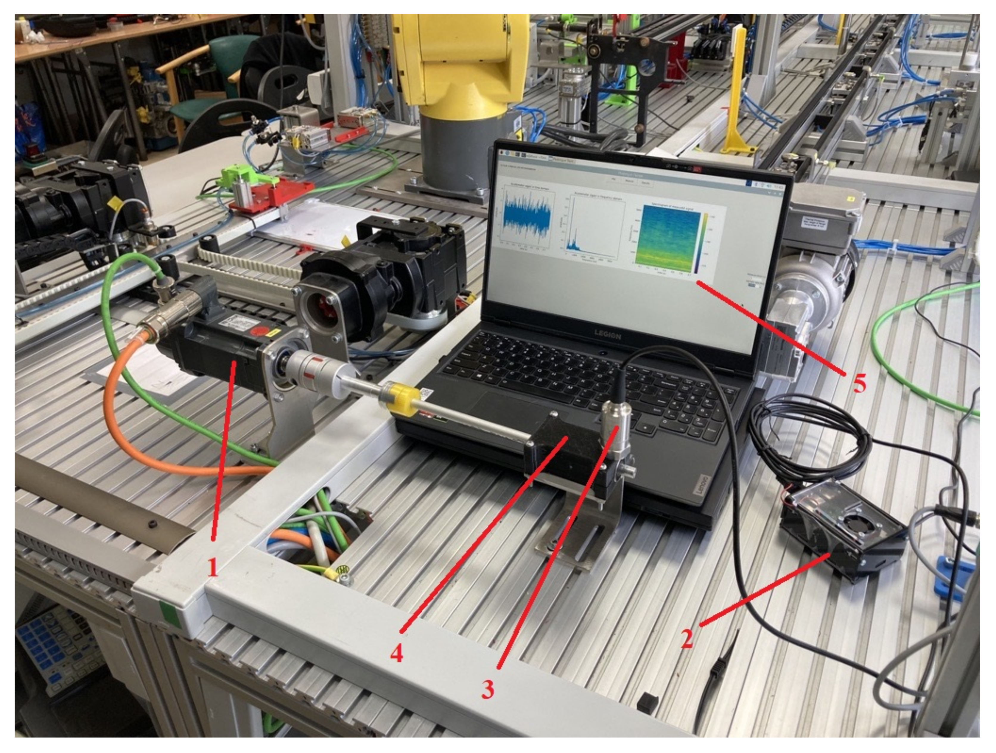
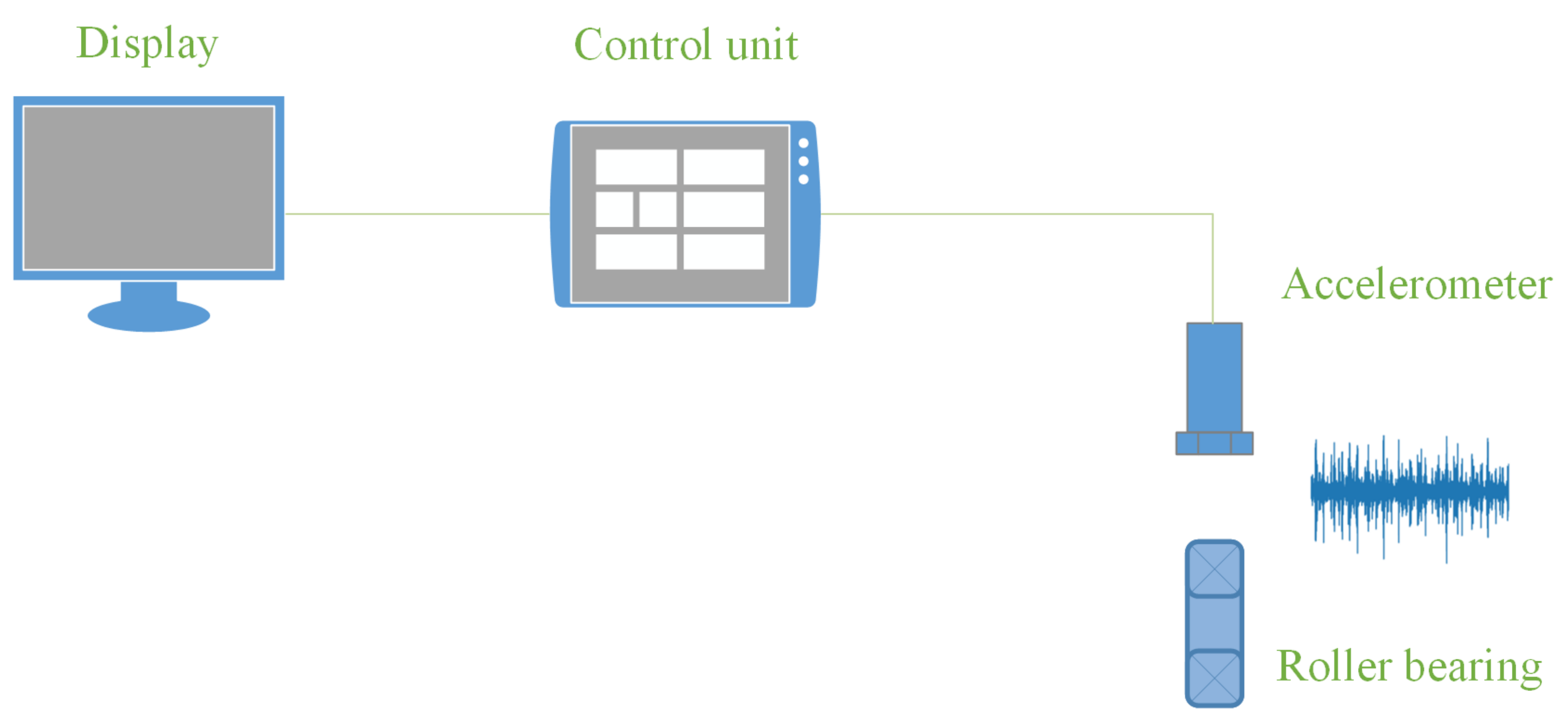
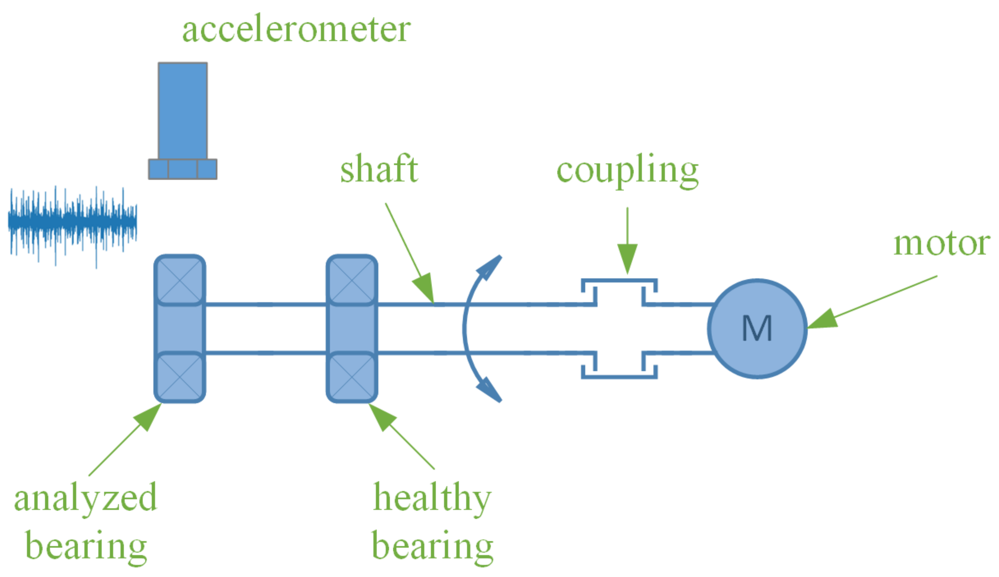
4. Measurement Stand
- linear ( 5%) frequency response from 2 to 8000 Hz,
- a transducer with a resolution of 16 or 24 bits,
- measurement range:
- –
- channel A 196 m/s2
- –
- channel B 98 m/s2
- sensitivity:
- –
- channel A 4% FSV/g (Full Scale Value)
- –
- channel B 7.96% FSV/g
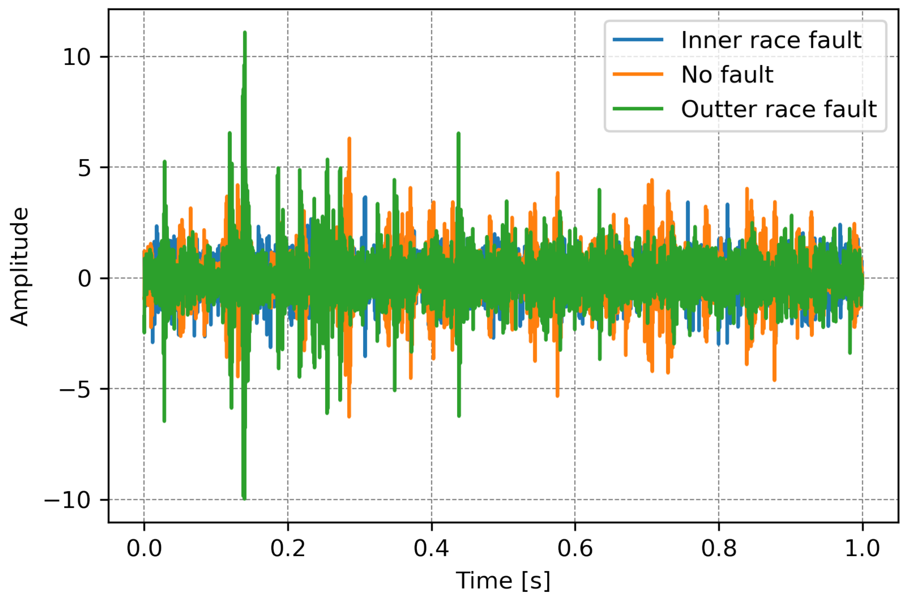
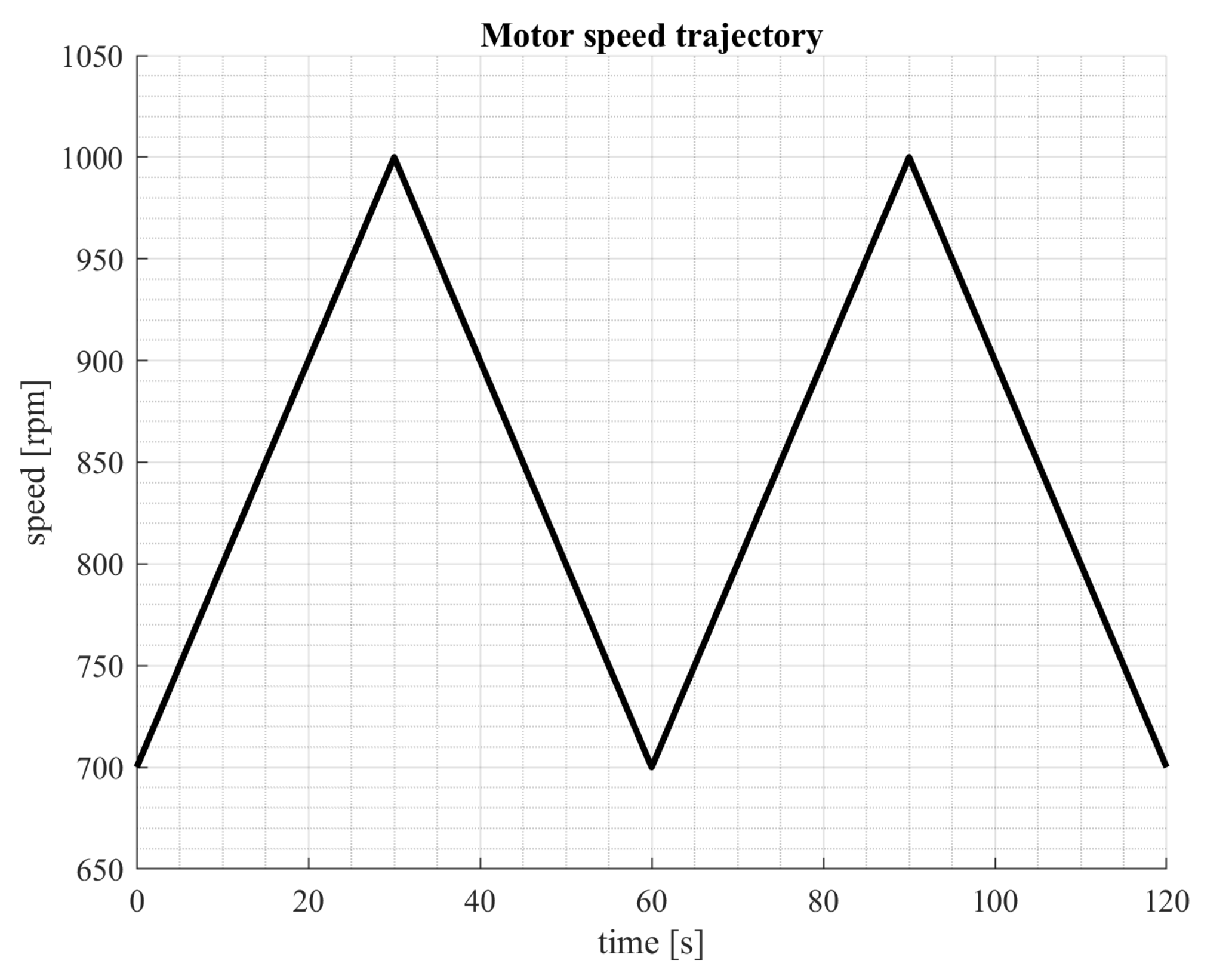
5. Data Acquisition
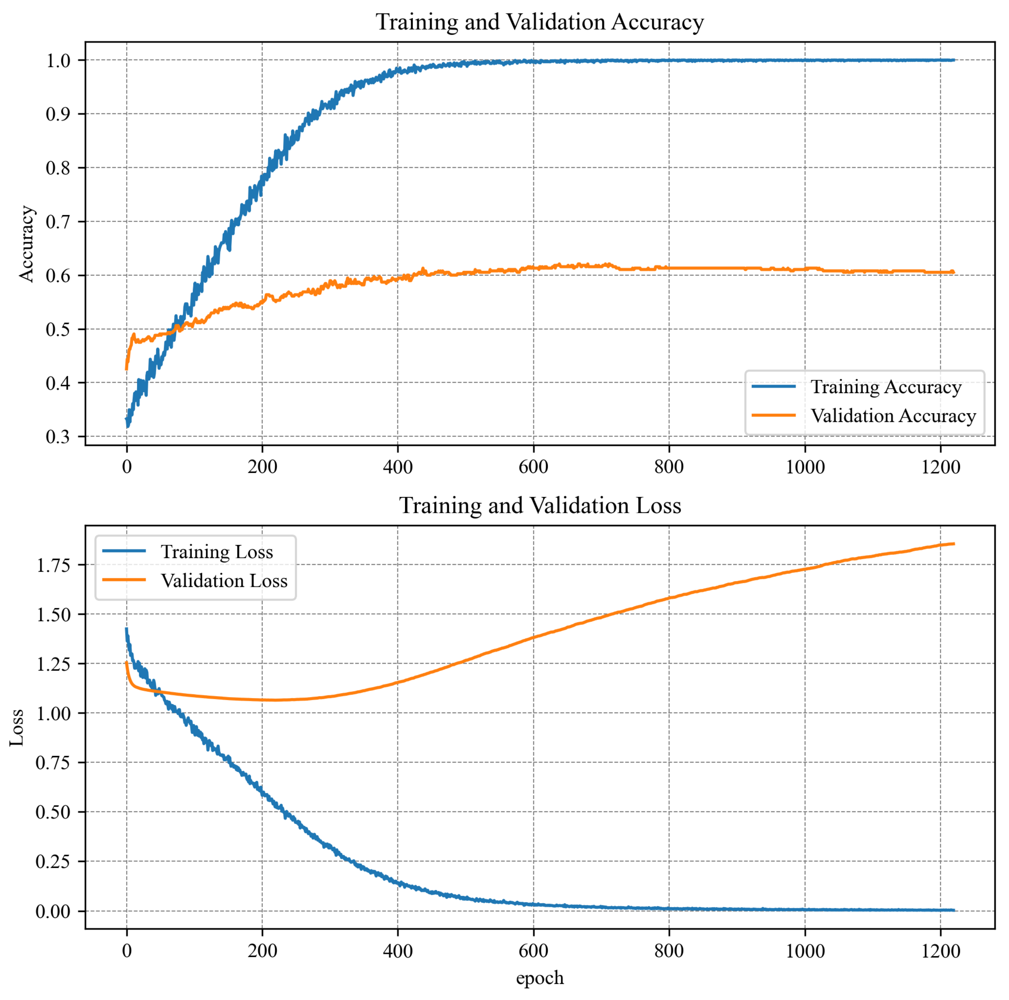
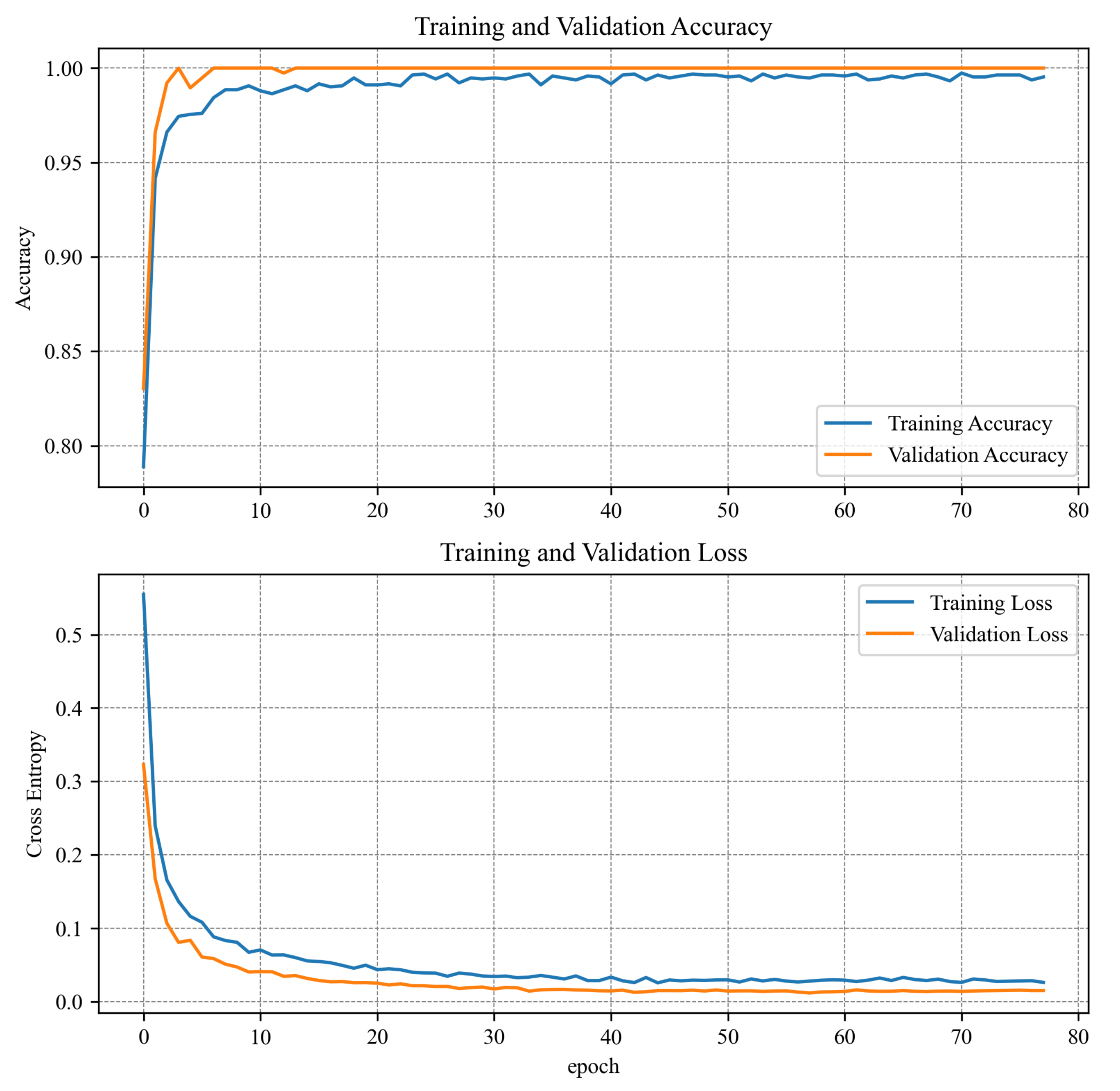
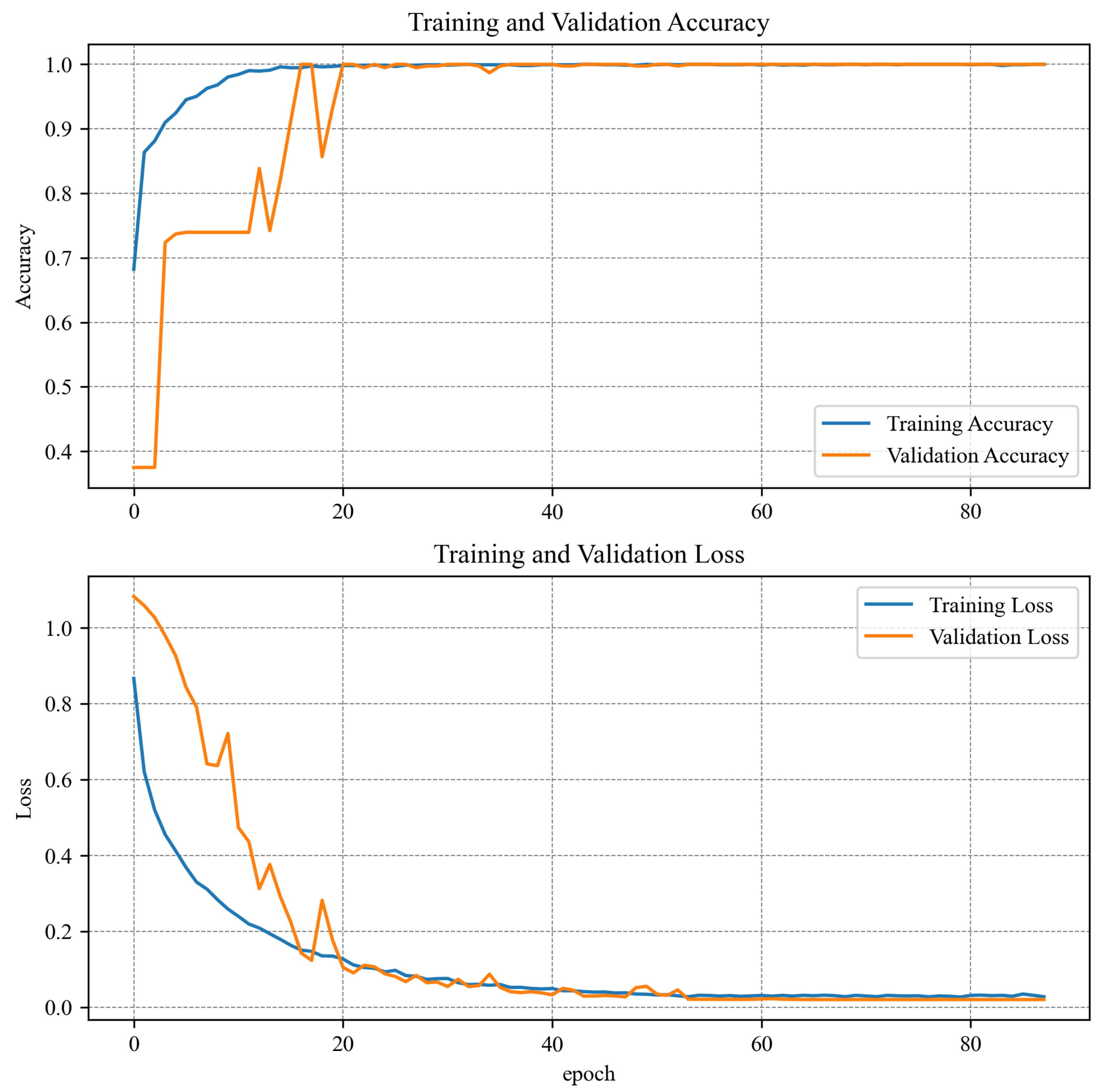
6. Training Results
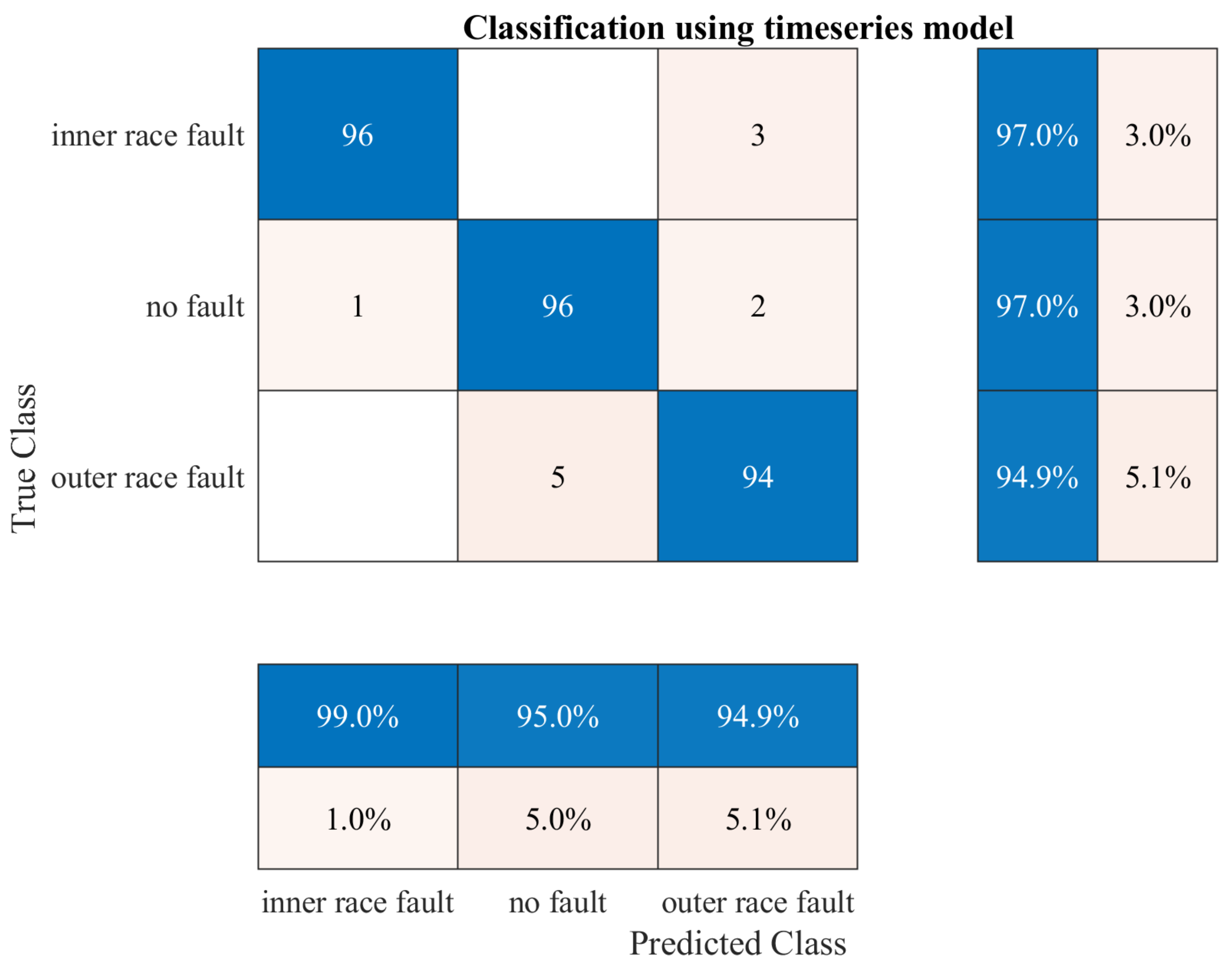
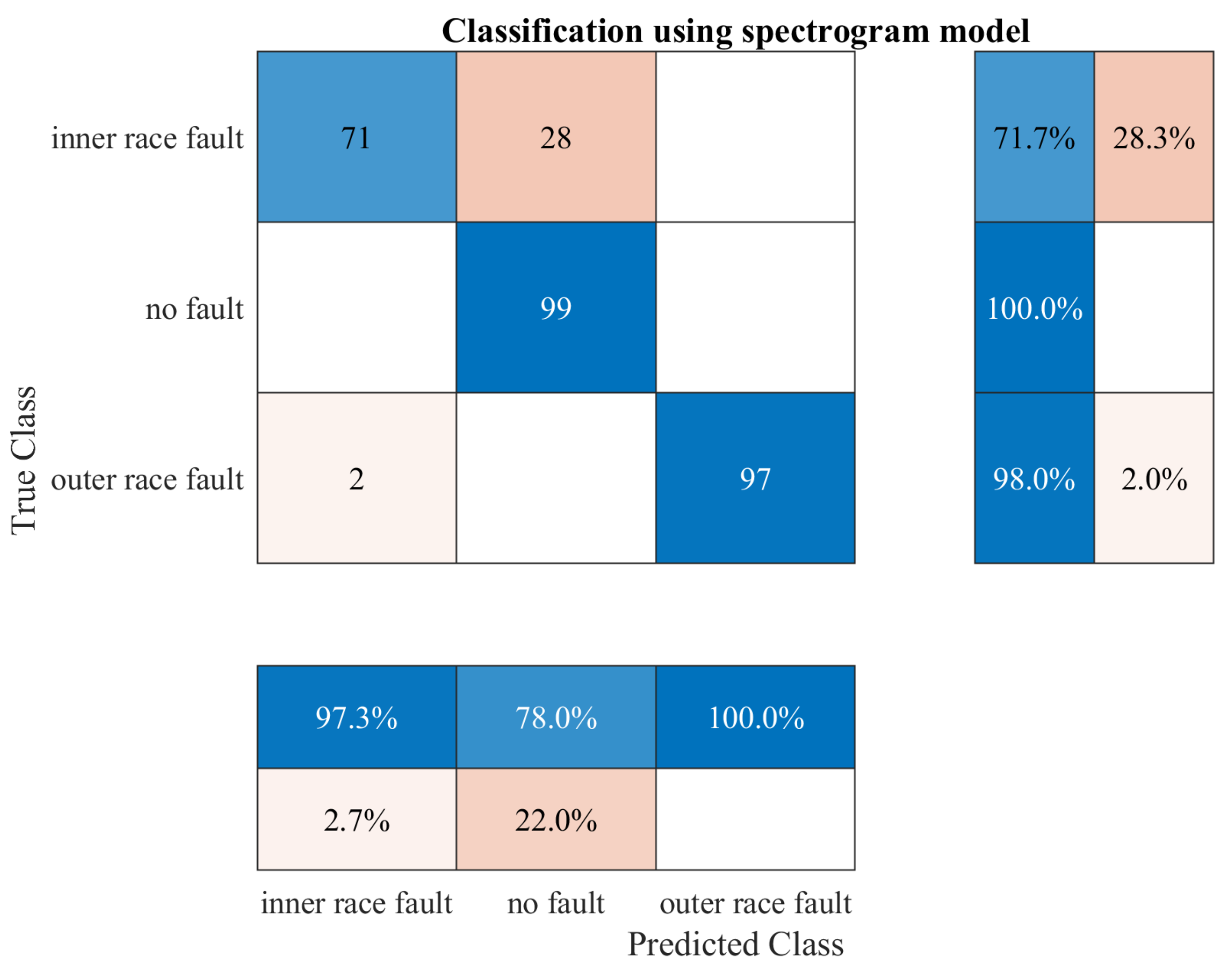
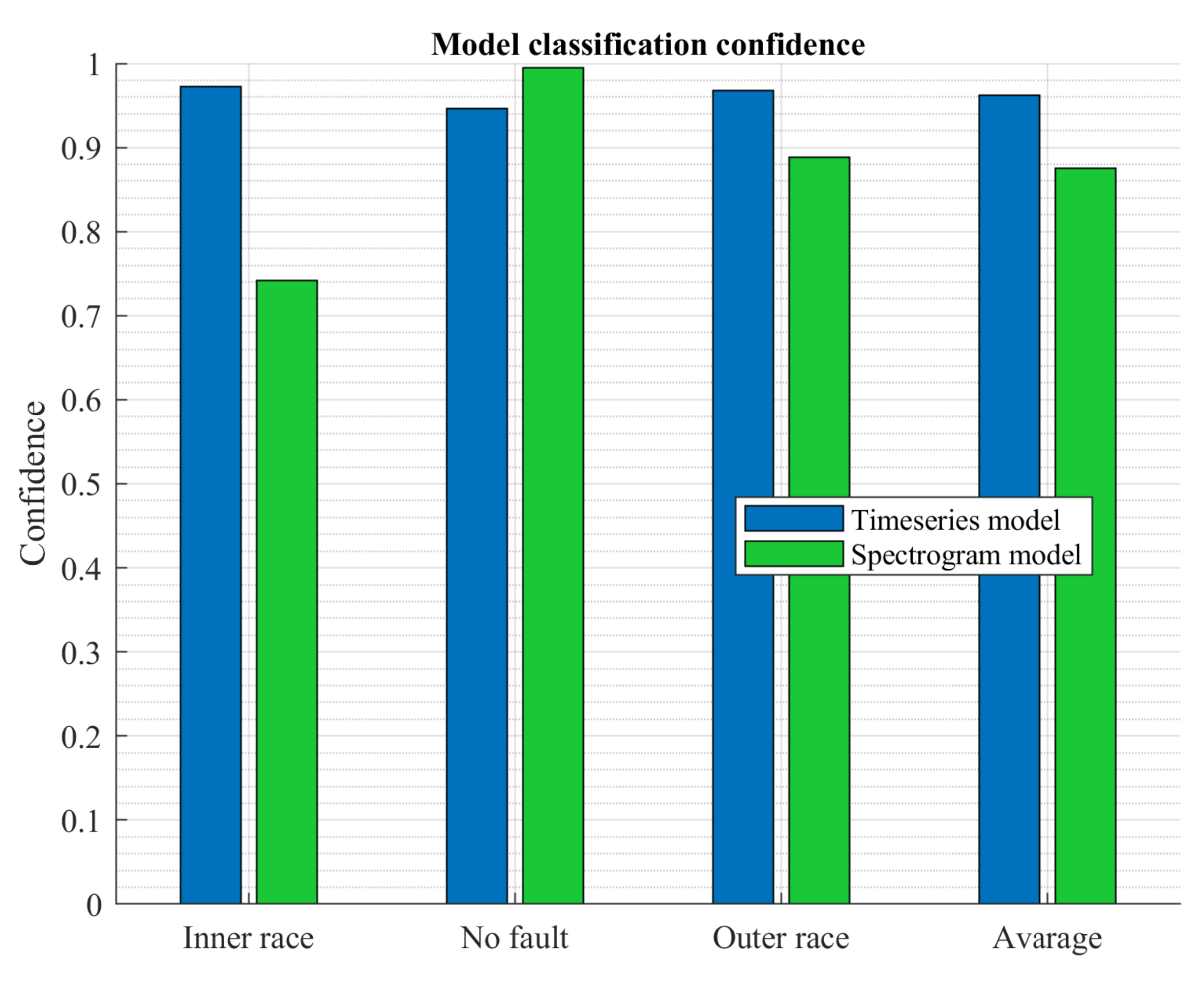
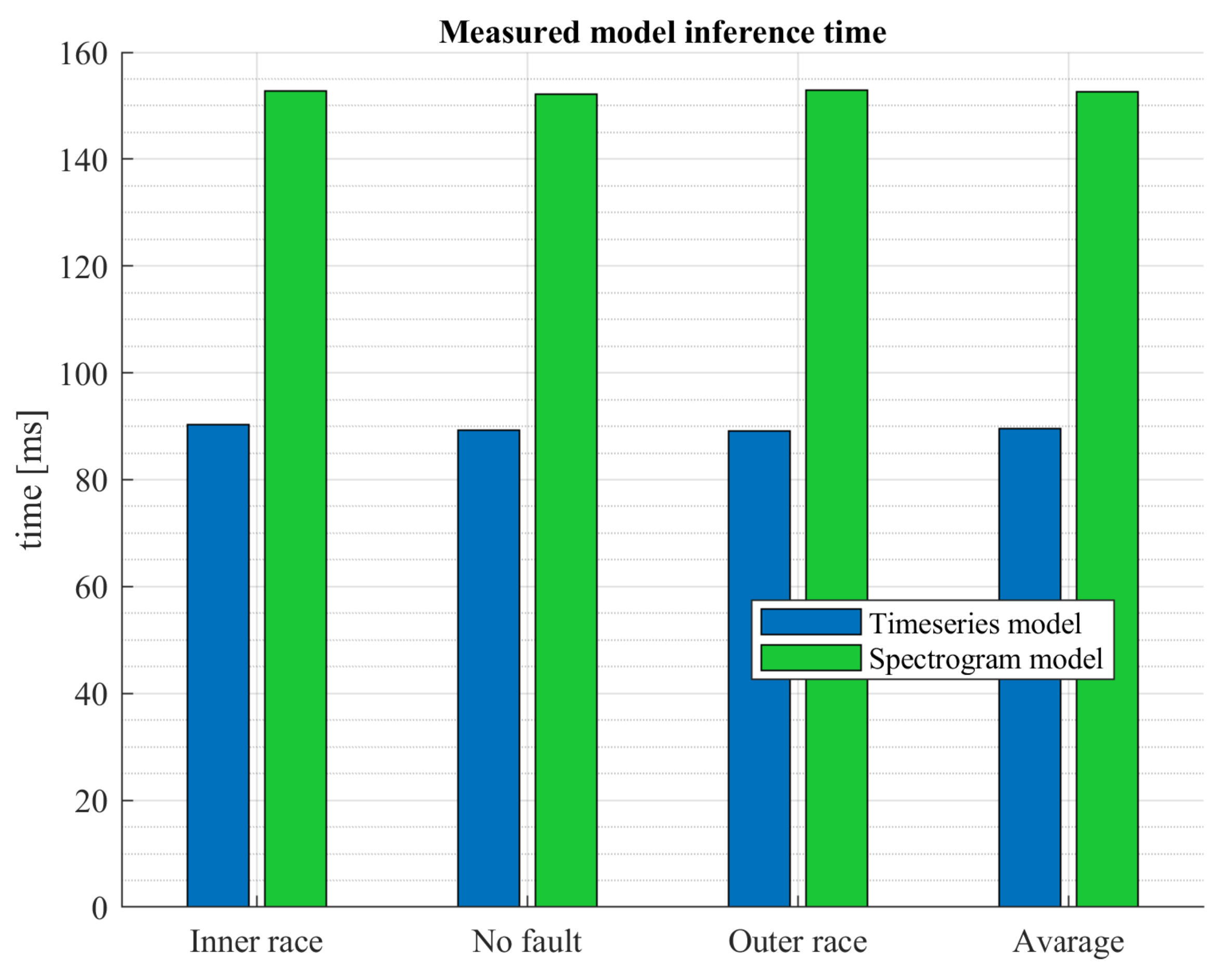
7. Testing Results
8. Conclusions
- average algorithm execution time reduced by 42% (64 ms)
- avarage precision during real time tests increased by 5.7%
- avarage confidence during real time tests increased by 8%
Author Contributions
Funding
Institutional Review Board Statement
Informed Consent Statement
Data Availability Statement
Conflicts of Interest
Abbreviations
| FFT | Fast Fourier Transform |
| CWT | Continuous Wavelet Transform |
| STFT | Short-Time Fourier Transform |
| RNN | Recurrent Neural Networks |
| SVM | Support Vector Machines |
| EEMD | Ensemble Empirical Mode Decomposition |
| WHT | Walsh-Hadamard Transform |
| DWT | Discrete Wavelet Transform |
| CNN | Convolutional Neural Network |
| SWD | Swarm Decomposition |
| BAS | Beetle Antennae Search |
| HDAN | hybrid distance-guided adversarial network |
| k-NN | k-Nearest Neighbours |
| AI | Artificial Intelligence |
| BPFO | Ball Pass Frequency of the Outer race |
| BPFI | Ball Pass Frequency of the Inner race |
| RELU | Rectified Linear Unit |
| MLP | Multilayer Perceptron |
| PLC | Programmable Logic Controller |
| SGD | Stochastic Gradient Descent |
| ADAM | Adaptive Moment Estimation |
| 1D | One-dimensional |
| 2D | Two-dimensional |
References
- Bechhoefer, E.; Kingsley, M.; Menon, P. Bearing envelope analysis window selection using spectral kurtosis techniques. In Proceedings of the 2011 IEEE Conference on Prognostics and Health Management, Denver, CO, USA, 20–23 June 2011; pp. 1–6. [Google Scholar]
- Cheng, C.; Zhang, B.k.; Gao, D. A predictive maintenance solution for bearing production line based on edge-cloud cooperation. In Proceedings of the 2019 Chinese Automation Congress (CAC), Hangzhou, China, 22–24 November 2019; pp. 5885–5889. [Google Scholar]
- Silvestrin, L.P.; Hoogendoorn, M.; Koole, G. A Comparative Study of State-of-the-Art Machine Learning Algorithms for Predictive Maintenance. In Proceedings of the SSCI, Xiamen, China, 6–9 December 2019; pp. 760–767. [Google Scholar]
- Serradilla, O.; Zugasti, E.; Rodriguez, J.; Zurutuza, U. Deep learning models for predictive maintenance: A survey, comparison, challenges and prospects. Appl. Intell. 2022, 52, 10934–10964. [Google Scholar] [CrossRef]
- Karakose, M.; Yaman, O. Complex fuzzy system based predictive maintenance approach in railways. IEEE Trans. Ind. Inform. 2020, 16, 6023–6032. [Google Scholar] [CrossRef]
- Dominik, I. Type-2 fuzzy logic controller for position control of shape memory alloy wire actuator. J. Intell. Mater. Syst. Struct. 2016, 27, 1917–1926. [Google Scholar] [CrossRef]
- Dominik, I.; Iwaniec, M.; Lech, Ł. Low frequency damage analysis of electric pylon model by fuzzy logic application. J. Low Freq. Noise Vib. Act. Control 2013, 32, 239–251. [Google Scholar] [CrossRef]
- Tao, H.; Wang, P.; Chen, Y.; Stojanovic, V.; Yang, H. An unsupervised fault diagnosis method for rolling bearing using STFT and generative neural networks. J. Frankl. Inst. 2020, 357, 7286–7307. [Google Scholar] [CrossRef]
- Pham, M.T.; Kim, J.M.; Kim, C.H. Accurate bearing fault diagnosis under variable shaft speed using convolutional neural networks and vibration spectrogram. Appl. Sci. 2020, 10, 6385. [Google Scholar] [CrossRef]
- Chen, H.Y.; Lee, C.H. Vibration signals analysis by explainable artificial intelligence (XAI) approach: Application on bearing faults diagnosis. IEEE Access 2020, 8, 134246–134256. [Google Scholar] [CrossRef]
- Rivera, D.L.; Scholz, M.R.; Fritscher, M.; Krauss, M.; Schilling, K. Towards a predictive maintenance system of a hydraulic pump. IFAC-PapersOnLine 2018, 51, 447–452. [Google Scholar] [CrossRef]
- Pech, M.; Vrchota, J.; Bednář, J. Predictive maintenance and intelligent sensors in smart factory. Sensors 2021, 21, 1470. [Google Scholar] [CrossRef]
- Vasilić, P.; Vujnović, S.; Popović, N.; Marjanović, A.; Đurović, Ž. Adaboost algorithm in the frame of predictive maintenance tasks. In Proceedings of the 2018 23rd International Scientific-Professional Conference on Information Technology (IT), Zabljak, Montenegro, 19–24 February 2018; pp. 1–4. [Google Scholar]
- Wu, H.; He, J.; Tömösközi, M.; Fitzek, F.H. Abstraction-based Multi-object Acoustic Anomaly Detection for Low-complexity Big Data Analysis. In Proceedings of the 2021 IEEE International Conference on Communications Workshops (ICC Workshops), Montreal, QC, Canada, 14–23 June 2021; pp. 1–6. [Google Scholar]
- Massaro, A.; Manfredonia, I.; Galiano, A.; Pellicani, L.; Birardi, V. Sensing and quality monitoring facilities designed for pasta industry including traceability, image vision and predictive maintenance. In Proceedings of the 2019 II Workshop on Metrology for Industry 4.0 and IoT (MetroInd4. 0&IoT), Naples, Italy, 4–6 June 2019; pp. 68–72. [Google Scholar]
- Khajavi, S.H.; Motlagh, N.H.; Jaribion, A.; Werner, L.C.; Holmström, J. Digital twin: Vision, benefits, boundaries, and creation for buildings. IEEE Access 2019, 7, 147406–147419. [Google Scholar] [CrossRef]
- Sambhi, S. Thermal Imaging Technology for Predictive Maintenance of Electrical Installation in Manufacturing Plant—A Literature Review. In Proceedings of the 2nd IEEE International Conference on Power Electronics, Intelligent Control and Energy Systems (ICPEICES-2018), Delhi, India, 22–24 October 2018. [Google Scholar]
- Pinto, R.; Cerquitelli, T. Robot fault detection and remaining life estimation for predictive maintenance. Procedia Comput. Sci. 2019, 151, 709–716. [Google Scholar] [CrossRef]
- Xu, G.; Liu, M.; Wang, J.; Ma, Y.; Wang, J.; Li, F.; Shen, W. Data-driven fault diagnostics and prognostics for predictive maintenance: A brief overview. In Proceedings of the 2019 IEEE 15th international conference on automation science and engineering (CASE), Vancouver, BC, Canada, 22–26 August 2019; pp. 103–108. [Google Scholar]
- Frangopol, D.M.; Kallen, M.J.; Noortwijk, J.M.V. Probabilistic models for life-cycle performance of deteriorating structures: Review and future directions. Prog. Struct. Eng. Mater. 2004, 6, 197–212. [Google Scholar] [CrossRef]
- Endrenyi, J.; Aboresheid, S.; Allan, R.; Anders, G.; Asgarpoor, S.; Billinton, R.; Chowdhury, N.; Dialynas, E.; Fipper, M.; Fletcher, R.; et al. The present status of maintenance strategies and the impact of maintenance on reliability. IEEE Trans. Power Syst. 2001, 16, 638–646. [Google Scholar] [CrossRef]
- Rahhal, J.S.; Abualnadi, D. IOT based predictive maintenance using LSTM RNN estimator. In Proceedings of the 2020 International Conference on Electrical, Communication, and Computer Engineering (ICECCE), Istanbul, Turkey, 12–13 June 2020; pp. 1–5. [Google Scholar]
- Sreejith, B.; Verma, A.; Srividya, A. Fault diagnosis of rolling element bearing using time-domain features and neural networks. In Proceedings of the 2008 IEEE Region 10 and the Third International Conference on Industrial and Information Systems, Kharagpur, India, 8–10 December 2008; pp. 1–6. [Google Scholar]
- Srinivasan, V.; Eswaran, C.; Sriraam, A.N. Artificial neural network based epileptic detection using time-domain and frequency-domain features. J. Med Syst. 2005, 29, 647–660. [Google Scholar] [CrossRef]
- Kovalev, D.; Shanin, I.; Stupnikov, S.; Zakharov, V. Data mining methods and techniques for fault detection and predictive maintenance in housing and utility infrastructure. In Proceedings of the 2018 International Conference on Engineering Technologies and Computer Science (EnT), Moscow, Russia, 20–21 March 2018; pp. 47–52. [Google Scholar]
- Dave, V.; Singh, S.; Vakharia, V. Diagnosis of bearing faults using multi fusion signal processing techniques and mutual information. Indian J. Eng. Mater. Sci. (IJEMS) 2021, 27, 878–888. [Google Scholar]
- Wang, J.; Wang, D.; Wang, S.; Li, W.; Song, K. Fault Diagnosis of Bearings Based on Multi-Sensor Information Fusion and 2D Convolutional Neural Network. IEEE Access 2021, 9, 23717–23725. [Google Scholar] [CrossRef]
- Wang, H.; Sun, W.; He, L.; Zhou, J. Rolling Bearing Fault Diagnosis Using Multi-Sensor Data Fusion Based on 1D-CNN Model. Entropy 2022, 24, 573. [Google Scholar] [CrossRef]
- Han, B.; Ji, S.; Wang, J.; Bao, H.; Jiang, X. An intelligent diagnosis framework for roller bearing fault under speed fluctuation condition. Neurocomputing 2021, 420, 171–180. [Google Scholar] [CrossRef]
- Han, B.; Zhang, X.; Wang, J.; An, Z.; Jia, S.; Zhang, G. Hybrid distance-guided adversarial network for intelligent fault diagnosis under different working conditions. Measurement 2021, 176, 109197. [Google Scholar] [CrossRef]
- Konieczny, J.; Stojek, J. Use of the K-Nearest Neighbour Classifier in Wear Condition Classification of a Positive Displacement Pump. Sensors 2021, 21, 6247. [Google Scholar] [CrossRef]
- Kwaśniewki, J.; Dominik, I.; Lalik, K.; Holewa, K. Influence of acoustoelastic coefficient on wave time of flight in stress measurement in piezoelectric self-excited system. Mech. Syst. Signal Process. 2016, 78, 143–155. [Google Scholar] [CrossRef]
- Carvalho, T.P.; Soares, F.A.; Vita, R.; Francisco, R.d.P.; Basto, J.P.; Alcalá, S.G. A systematic literature review of machine learning methods applied to predictive maintenance. Comput. Ind. Eng. 2019, 137, 106024. [Google Scholar] [CrossRef]
- Książek, M.A.; Ziemiański, D. Optimal driver seat suspension for a hybrid model of sitting human body. J. Terramechanics 2012, 49, 255–261. [Google Scholar] [CrossRef]
- Ran, Y.; Zhou, X.; Lin, P.; Wen, Y.; Deng, R. A survey of predictive maintenance: Systems, purposes and approaches. arXiv 2019, arXiv:1912.07383. [Google Scholar]
- Saucedo-Dorantes, J.J.; Zamudio-Ramirez, I.; Cureno-Osornio, J.; Osornio-Rios, R.A.; Antonino-Daviu, J.A. Condition Monitoring Method for the Detection of Fault Graduality in Outer Race Bearing Based on Vibration-Current Fusion, Statistical Features and Neural Network. Appl. Sci. 2021, 11, 8033. [Google Scholar] [CrossRef]
- Sandler, M.; Howard, A.; Zhu, M.; Zhmoginov, A.; Chen, L.C. MobileNetV2: Inverted Residuals and Linear Bottlenecks. In Proceedings of the 2018 IEEE/CVF Conference on Computer Vision and Pattern Recognition (CVPR), Salt Lake City, UT, USA, 18–23 June 2018. [Google Scholar] [CrossRef]
- Fawaz, H.I.; Forestier, G.; Weber, J.; Idoumghar, L.; Muller, P. Deep learning for time series classification: A review. Data Min. Knowl. Discov. 2019, 33, 917–963. [Google Scholar] [CrossRef]
- Wang, Z.; Yan, W.; Oates, T. Time Series Classification from Scratch with Deep Neural Networks: A Strong Baseline. arXiv 2016, arXiv:1611.06455. [Google Scholar] [CrossRef]
- He, K.; Zhang, X.; Ren, S.; Sun, J. Deep Residual Learning for Image Recognition. In Proceedings of the IEEE Conference on Computer Vision and Pattern Recognition (CVPR), Las Vegas, NV, USA, 27–30 June 2016. [Google Scholar]
- Bagnall, A.; Lines, J.; Bostrom, A.; Large, J.; Keogh, E. The great time series classification bake off: A review and experimental evaluation of recent algorithmic advances. Data Min. Knowl. Discov. 2017, 31, 606–660. [Google Scholar] [CrossRef]
- Oppenheim, A.; Schafer, R.; Buck, J.; Lee, L. Discrete-Time Signal Processing; Prentice Hall International Editions; Prentice Hall: Hoboken, NJ, USA, 1999. [Google Scholar]


| Input | Operator | Output |
|---|---|---|
| 3 × 3 dwise s = s, ReLU6 | ||
| 1 × 1 conv2d, ReLU6 | ||
| linear 1 × 1, conv2d |
| Operator | Output |
|---|---|
| input layer | |
| MobileNet-v2 body | |
| GlobalAveragePooling2D | |
| Dropout | |
| Dense | |
| Softmax | |
| Model | Non-Trainable | Trainable | Total |
|---|---|---|---|
| Spectrogram | 2,257,984 | 3843 | 2,261,827 |
| 4 conv blocks | 512 | 38,019 | 38,531 |
| 3 conv blocks | 384 | 25,539 | 25,923 |
| MLP | 0 | 6,015,503 | 6,015,503 |
| Parameter | Spectrogram | Time Series CNN | Time Series MLP |
|---|---|---|---|
| Training loss | 0.0278 | 0.0279 | 0.0028 |
| Training accuracy | 96.43% | 97.26% | 99.93% |
| Validation loss | 0.0144 | 0.0206 | 1.8550 |
| Validation accuracy | 97.76% | 99.32% | 60.52% |
| Epochs | 78 | 88 | 1220 |
Disclaimer/Publisher’s Note: The statements, opinions and data contained in all publications are solely those of the individual author(s) and contributor(s) and not of MDPI and/or the editor(s). MDPI and/or the editor(s) disclaim responsibility for any injury to people or property resulting from any ideas, methods, instructions or products referred to in the content. |
© 2023 by the authors. Licensee MDPI, Basel, Switzerland. This article is an open access article distributed under the terms and conditions of the Creative Commons Attribution (CC BY) license (https://creativecommons.org/licenses/by/4.0/).
Share and Cite
Knap, P.; Lalik, K.; Bałazy, P. Boosted Convolutional Neural Network Algorithm for the Classification of the Bearing Fault form 1-D Raw Sensor Data. Sensors 2023, 23, 4295. https://doi.org/10.3390/s23094295
Knap P, Lalik K, Bałazy P. Boosted Convolutional Neural Network Algorithm for the Classification of the Bearing Fault form 1-D Raw Sensor Data. Sensors. 2023; 23(9):4295. https://doi.org/10.3390/s23094295
Chicago/Turabian StyleKnap, Paweł, Krzysztof Lalik, and Patryk Bałazy. 2023. "Boosted Convolutional Neural Network Algorithm for the Classification of the Bearing Fault form 1-D Raw Sensor Data" Sensors 23, no. 9: 4295. https://doi.org/10.3390/s23094295
APA StyleKnap, P., Lalik, K., & Bałazy, P. (2023). Boosted Convolutional Neural Network Algorithm for the Classification of the Bearing Fault form 1-D Raw Sensor Data. Sensors, 23(9), 4295. https://doi.org/10.3390/s23094295