Graph Representation Learning and Its Applications: A Survey

Abstract

Graphs are data structures that effectively represent relational data in the real world. Graph representation learning is a significant task since it could facilitate various downstream tasks, such as node classification, link prediction, etc. Graph representation learning aims to map graph entities to low-dimensional vectors while preserving graph structure and entity relationships. Over the decades, many models have been proposed for graph representation learning. This paper aims to show a comprehensive picture of graph representation learning models, including traditional and state-of-the-art models on various graphs in different geometric spaces. First, we begin with five types of graph embedding models: graph kernels, matrix factorization models, shallow models, deep-learning models, and non-Euclidean models. In addition, we also discuss graph transformer models and Gaussian embedding models. Second, we present practical applications of graph embedding models, from constructing graphs for specific domains to applying models to solve tasks. Finally, we discuss challenges for existing models and future research directions in detail. As a result, this paper provides a structured overview of the diversity of graph embedding models.

1. Introduction

Graphs are a common language for representing complex relational data, including social media, transportation system networks, and biological protein–protein networks [1,2]. Since most graph data are complex and high-dimensional, it is difficult for researchers to extract valuable knowledge. Therefore, processing graph data and transforming them into a form (fixed-dimensional vectors) is an important process that researchers can then apply to different downstream tasks [3]. The objective of graph representation learning is to obtain vector representations of graph entities (e.g., nodes, edges, subgraphs, etc.) to facilitate various downstream tasks, such as node classification [4], link prediction [5,6], community detection [7], etc. As a result, graph representation learning plays an important role since it could significantly promote the performance of the downstream tasks.

Representation of the graph data, however, is challenging and different from image and text data [8]. In textual data, words are linked together in a sentence, and they have a fixed position in that sentence. In image data, pixels are arranged on an ordered grid space and can be represented by a grid matrix. However, the nodes and edges in graphs are non-ordered and have their features. This leads to mapping graph entities to latent space while preserving the graph structure, and proximity relationships are challenging. In the case of a social network, a user can have many friends (neighbors) and various personal information, such as hometown, education level, and hobbies, which makes preserving the graph structure and properties significantly problematic. In addition, many real-world networks show dynamic behaviors in which graph structures and node features could be changed over time [9,10]. These could deliver challenges in capturing the graph structure and mapping graph entities into vector space.

Over decades, various graph representation learning models have been proposed to project graph entities into fixed-length vectors [11,12,13]. Graph embedding models are mainly divided into five main groups: graph kernels, matrix factorization models, shallow models, deep neural network models, and non-Euclidean models. Figure 1 presents the popularity of different graph representation learning models from 2010 to 2022. The number of graph representation learning studies increased considerably over the period of 12 years. Furthermore, there was significant growth in the frequency of research studies on graph neural networks, graph convolutional networks, and graph transformer models. In contrast, the number of studies in graph kernels, graph autoencoder, and matrix factorization-based models increased slightly over the period of 12 years. We obtained the frequency of academic publications including each keyword from Scopus (https://www.scopus.com (accessed on 16 April 2023)).

Historically, the first graph representation learning models were graph kernels. The idea of graph kernel methods perhaps comes from the most essential and well-known Weisfeiler–Lehman (WL) isomorphic testing in 1968 [31]. Graph kernels are kernel functions that aim to measure the similarity between graphs and their entities [32]. The main idea of graph kernels is to decompose original graphs into substructures and construct vector embeddings based on the substructure features. There are two main types of graph kernels: kernels for graphs and kernels on graphs. The former aims to measure the similarity between pairs of graphs, while the latter estimates the similarity between graph nodes. Several strategies to estimate the similarity of graph pairs have been proposed to represent various graph structures, such as graphlet kernels, random walk, and the shortest path, which started in the 2000s. Based on WL isomorphic testing, various graph kernels are built to compute the similarity of pairs of graph entities, such as WL kernels [31], WL subtree kernels [33,34,35], and random walks [36,37]. However, one of the limitations of graph kernels is the computational complexity when working with large-scale graphs since computing graph kernels is an NP-hard class.

Early models for graph representation learning primarily focused on matrix factorization methods, which are motivated by traditional techniques for dimensionality reduction in 2002 [38]. Several matrix factorization-based models have been proposed to handle large graphs with millions of nodes [39,40]. The objective of matrix factorization models is to decompose the proximity matrix into a product of small-sized matrices and then learn the embeddings that fit the proximity. Based on the ways to learn vector embeddings, there are two main lines of matrix factorization models: Laplacian eigenmaps and node proximity matrix factorization. Starting in the 2000s, Laplacian eigenmaps methods [41,42] aim to represent each node by Laplacian eigenvectors along with the first k eigenvalues. In contrast, the node proximity matrix factorization methods [5,15] aim to gain node embeddings by the singular value decomposition in 2015. Various proximity matrix factorization models have successfully handled large graphs and achieved great performance [15,43]. However, matrix factorization models suffer from capturing high-order proximity due to computational complexity when performing with high transition matrices.

In 2014 and 2016, early shallow models, DeepWalk [14] and Node2Vec [4] were proposed, which learn node embeddings based on shallow neural networks. Remarkably, the primary concept is to learn node embeddings by maximizing the neighborhood probability of target nodes using the skip-gram model started in the natural language processing area. The purpose of this strategy could then be optimized with SGD on neural network layers, thus reducing computational complexity. With this historic milestone, various models have been developed by improving multiple sampling strategies and training processes. Shallow models are the embedding models that aim to map graph entities to low-dimensional vectors by conducting an embedding lookup for each graph entity [3]. From this perspective, the embedding of node $v_i$ could be represented as $Z_i=M{x}_i$, where M denotes an embedding matrix of all nodes and $x_i$ is a one-hot vector of node $v_i$. Various shallow models have been proposed to learn embeddings with different strategies to preserve graph structures and the similarity between graph entities. Structure-preservation models aim to preserve the structural connection between entities (e.g., DeepWalk [14], Node2Vec [4]). In 2015, Tang et al. [16] proposed the LINE model, a proximity reconstruction method that aims to preserve proximity between nodes in graphs. After that, various models have been proposed to preserve the node proximity with higher-order proximity and capture more global graph structure. However, most of the above models focus on transductive learning and ignore node features, which may have several limitations to practical applications.

Breakthroughs in deep learning have led to a new research perspective on applying deep neural networks to the graph domain. Since the 2000s, there have been several early models on GNNs designed to learn node embeddings based on neighborhood information using an aggregation mechanism [44,45]. Graph neural networks (GNNs) have shown a significant expressive capacity to represent graph embeddings in an inductive learning manner and solve the limitations of aforementioned shallow models [46,47]. Recurrent GNNs are also the first studies on GNNs based on recurrent neural network architecture [48,49] in 2005. These models aim to learn node embeddings via recurrent layers with the same weights in each hidden layer and run recursively until convergence. Several recurrent GNNs with different strategies have been proposed by the power of recurrent neural network architecture and the combinations with several sampling strategies. However, using the same weights at each hidden layer of the RGNN model may cause the model to be incapable of distinguishing the local and global structure. Since 2016, several graph autoencoder models have been proposed based on the original autoencoder architecture, which could learn complex graph structures by reconstructing the input graph structure [50,51]. The graph autoencoders comprise two main layers: encoder layers take the adjacency matrix as input and squeeze it to generate node embeddings, and decoder layers reconstruct the input data. By contrast, the idea of CGNNs is to use convolutional operators with different weights in each hidden layer, which are more efficient in capturing and distinguishing the local and global structures [18,52,53,54]. Many studies have been proposed with various variants of CGNNs, including spectral CGNNs [55,56,57] started in 2014, spatial CGNNs [22,24,52] started in 2016, and attentive CGNNs [19,58] started in 2017. Nevertheless, most GNNs suffer limitations such as over-smoothing problems and noise from neighbor nodes when stacking more GNN layers [59,60].

Motivated by transformer architecture started from natural language processing applications in 2017, several graph transformer models were proposed using the transformer architecture to the graph domain in 2019 [61,62]. Graph transformer models have shown competitive and superior performance against GNNs in learning complex graph structures [30,63]. Graph transformer models can be divided into three main groups: transformer for tree-like graphs, transformer with GNNs, and transformer with global self-attention. Early graph transformer models aim to learn tree-like graphs, which mainly aim at learning node embeddings in tree-like graphs where nodes are arranged hierarchically [64,65] since 2019. These models encode the node positions through their relative and absolute positional encoding in trees as constraints with root nodes and neighbor nodes at the same level. Second, several models leverage the power of GNNs as an auxiliary module in computing attention scores [66]. In addition, some models put GNN layers on top of the model to overcome the over-smoothing problem and make the model remember the local structure [61]. Most above graph transformer models adopt vanilla transformer architecture to learn embeddings that rely on multi-head self-attention. Third, several graph transformer models use a global self-attention mechanism to learn node embeddings, which implements self-attention independently and does not require constraints from the neighborhood [30,67]. These models work directly on input graphs and can capture the global structure with global self-attention.

Most of the above models learn embeddings in Euclidean space and represent graph entities as vector points in latent space. However, graphs in the real world could have complex structures and different forms, such that Euclidean space may be inadequate to represent the graph structure and ultimately lead to structural loss [68,69]. Early models learn complex graphs in non-Euclidean geometry by developing efficient algorithms for learning node embeddings based on manifold optimization [70] in 2017. Following the line, several models aim to represent graph data in non-Euclidean space and gain desirable results [68,69,71]. Two typical non-Euclidean spaces, including spherical and hyperbolic geometry, have their advantages. Spherical space could represent graph structures with large cycles, while hyperbolic space is suitable for hierarchical graph structures. Most non-Euclidean models aim to design an efficient algorithm for learning node embeddings since it is challenging to implement operators directly in non-Euclidean. Furthermore, to deal with uncertainty, several Gaussian graph models have been introduced to represent graph entities as density-based embeddings [23] started in 2016. Node embeddings could be defined as a continuous density mostly based on Gaussian distribution [72].

To the extent of our knowledge, no comparable paper in the literature focuses on a wide range of graph embedding models for static and dynamic graphs in different geometric spaces. Most current papers only presented specific approaches for graph representation learning. Wu et al. [8] focused on graph neural network models, which are presented as a section in this paper. Several surveys [13,73,74] summarized graph embedding models for various types of graphs, but they did not mention either graph transformer models or non-Euclidean models. From applying graph embedding models to practical applications, several papers only list the applications for specific and narrow tasks [12,75]. However, we discuss how graphs are constructed in specific applications and how graph embedding models are implemented in various domains.

This paper presents a comprehensive picture of graph embedding models in static and dynamic graphs in different geometric spaces. In particular, we recognize five general categories of models for addressing graph representation learning, including graph kernels, matrix factorization models, shallow models, deep neural network models, and non-Euclidean models. The contribution of this study can be categorized as follows:

• This paper presents a taxonomy of graph embedding models based on various algorithms and strategies.
• We provide readers with an in-depth analysis of an overview of graph embedding models with different types of graphs ranging from static to dynamic and from homogeneous to heterogeneous graphs.
• This paper presents graph transformer models, which have achieved remarkable results in a deeper understanding of graph structures in recent years.
• We cover applications of graph representation learning in various areas, from constructing graphs to applying models in specific tasks.
• We discuss the challenges and future directions of existing graph embedding models in detail.

Since abundant graph representation learning models have been proposed recently, we employed different approaches to find related studies. We built a search strategy by defining keywords and analyzing reliable sources. The list of keywords includes graph embedding, graph representation learning, graph neural networks, graph convolution, graph attention, graph transformer, graph embedding in non-Euclidean space, Gaussian graph embedding, and applications of graph embedding. We found related studies at famous top-tier conferences and journals such as AAAI, IJCAI, SIGKDD, ICML, WSDM, Nature Machine Intelligence, Pattern Recognition, Intelligent Systems with Applications, the Web, and so on.

The following sections of this paper are summarized as follows. Section 2 describes fundamental concepts and backgrounds related to graph representation learning. In Section 3, all the graph embedding models will be presented, such as graph kernels, matrix factorization models, shallow models, deep neural network models, and non-Euclidean models. Section 4 discusses a wide range of practical applications of graph embedding models in the real world. Section 5 summarizes the latest benchmarks, downstream tasks, evaluation metrics, and libraries. Challenges for existing graph embedding models and future research directions will be discussed in Section 6. The last section, Section 7 is the conclusion.

2. Problem Description

Graph representation learning aims to project the graph entities into low-dimensional vectors while preserving the graph structure and the proximity of entities in graphs. With the desire to map graph entities into vector space, it is necessary to model the graph in mathematical form. Therefore, we begin with several fundamental definitions of graphs. The list of standard notations used in this survey is detailed in Table 1. Mathematically, a graph G can be defined as follows:

Definition 1

(Graph [3]). A graph is a discrete structure consisting of a set of nodes and the edges connecting those nodes. The graph can be described mathematically in the form: $G=(V,E,A)$, where $V=\{v_1,v_2,\cdots ,v_N\}$ is the set of nodes, $E=\left\{(v_i,v_j)\right|(v_i,v_j)\in V\times V\}$ is the set of edges, and A is an adjacency matrix. A is a square matrix of size $N\times N$ where N is the number of nodes in graphs. This can be formulated as follows:

 

$$\begin{array}{c}A=\left[\begin{array}{ccc}{A}_{11}& \cdots & A_{1N}\\ ⋮& \ddots & ⋮\\ A_{N1}& \cdots & A_{NN}\end{array}\right],A_{ij}=\left\{\begin{array}{cc}1,\hfill & if{e}_{ij}\in E.\hfill \\ 0,\hfill & otherwise.\hfill \end{array}\right.\end{array},$$

(1)

where $A_{ij}$ indicates adjacency between node $v_i$ and node $v_j$.

When $A_{ij}$ is binary, the matrix A represents only the existence of connections between nodes. By extending the definition of matrix A, we could expand to abundant different types of graph G:

• Directed graph: When $A_{ij}=A_{ji}$ for any $1\le i, j\le n$, then the graph G is called an undirected graph, and G is directed graph otherwise.
• Weighted graph: is a graph in which each edge is assigned a specific weight value. Therefore, the adjacency matrix could be presented as: $A_{ij}=w_{ij}$, where $w_{ij}\in \mathbb{R}$ is the weight of the edge $e_{ij}$.
• Signed graph: When $A_{ij}\in [-\infty ,\infty ]$, the graph G is called signature/signed graph. The graph G could have all positive signed edges when $A_{ij}>0$ for any $1\le i, j\le n$, and G could have all negative signed edges otherwise.
• Attributed graph: A graph $G=(V,E,A,X)$ is an attributed graph where V, E is the set of nodes and edges, respectively, and X is the matrix of node attributes with size $n\times d$. Furthermore, we could also have the matrix X as the matrix of edge input attribute with size $m\times d$ where m is the number of edges $e_{ij}\in E$ for any $1\le i, j\le n$.
• Hyper graph: A hyper graph G could be represented as $G=(V,E,W)$, where V denotes the set of nodes and E denotes a set of hyperedge. Each hyperedge $e_{ij}$ can connect multiple nodes and is assigned a weight $w_{ij}\in W$. The hypergraph G could be represented by an incidence matrix H size $\left|V\right|\times \left|E\right|$ with entries $h(v_i,v_j)=1$ if $e_{ij}\in E$, and $h(v_i,v_j)=0$ otherwise.
• Heterogeneous graph: A heterogeneous graph is defined as $G=(V,E,T,\phi ,\rho )$ where V, and E are the set of nodes and edges, respectively, $\phi$ is the mapping function: $\phi :V\to T_v$, and the mapping function $\rho :E\to T_e$ with $T_v$, $T_e$ describe the set of node types and edge types, respectively, and $T=T_v$+ $T_e$ is the sum of the number of node types and edge types.

According to the definitions of graph $G=(V,E)$ that have been represented mathematically above, the idea of graph embedding is to map graph entities into low-dimensional vectors with the number of dimensions d with $d\ll N$. Mathematically, the graph embedding is formulated as follows:

Definition 2

(Graph embedding [14]). Given a graph $G=(V,E)$ where V is the set of nodes, and E is the set of edges, graph embedding is a projection function $\varphi (·)$, where $\varphi :V\to {\mathbb{R}}^d$ ($d\ll \left|V\right|$) and $k(v_i,v_j)\simeq \langle \varphi \left(v_i\right),\varphi \left(v_j\right)\rangle$ describes the proximity of two nodes $v_i$ and $v_j$ in the graph and $\langle \varphi \left(v_i\right),\varphi \left(v_j\right)\rangle$ is the distance of two vectors $\varphi \left(v_i\right)$ and $\varphi \left(v_j\right)$ in the vector space.

Graph representation learning aims to project graph entities into the vector space while preserving the graph structure and entity proximity. For example, if two nodes $v_i$ and $v_j$ in the graph G are connected directly, then in vector space, the distance between two vectors $\varphi \left(v_i\right)$ and $\varphi \left(v_j\right)$ must be minimal. Figure 2 shows an example of a graph embedding model that transforms nodes in a graph to low-dimensional vectors $(Z_1{Z}_2\cdots Z_n)$ in the vector space.

When mapping graph entities to latent space, preserving the proximity of graph entities is one of the most important factors in preserving the graph structure and the relationship between nodes. In other words, if two nodes $v_i$ and $v_j$ are connected or close in the graph, the distance between the two vectors $Z_i$ and $Z_j$ must be minimal in the vector space. Several models [16,76,77,78] aim to preserve k-order proximity between graph entities in vector space. Formally, the k-order proximity is defined as follows:

Definition 3

(k-order proximity [79]). Given a graph $G=(V,E)$ where V is the set of nodes, and E is the set of edges, k-order proximity describes the similarity of nodes with the distance captured from the k-hop in the graph G. When $k=1$, it is 1st-order proximity that captures the local pairwise proximity of two nodes in graphs. When k is higher, it could capture the global graph structure.

There is another way to define graph embedding from the perspective of Encoder-Decoder architecture [3]. From this perspective, the task of the encoder part is to encode graph entities into low-dimensional vectors, and the decoder part tries to reconstruct the graph from the latent space. In the real world, many graphs show dynamic behaviors, including node and edge evolution, and feature evolution [80]. Dynamic graphs are found widely in many applications [81], such as social networks where connections between friends could be added or removed over time.

Definition 4

(Dynamic graph [80]). A dynamic graph $\mathbb{G}$ is formed of three entities: $\mathbb{G}=\left(\mathbb{V},\mathbb{E},T\right)$ where $\mathbb{V}=\left\{V\left(t\right)\right\}$ is the group of node sets, $\mathbb{E}=\left\{E\right(t\left)\right\}$ with $t\in T$ is the group of edge sets over time span T, and T denotes the time span. From the statistic perspective, we could also consider a dynamic graph $\mathbb{G}=\{G\left(t_0\right)G\left(t_1\right)\cdots G\left(t_n\right)\}$ as a collection of static graphs $G\left(t_k\right)$ where $G\left(t_k\right)=\left(V\left(t_k\right),E\left(t_k\right)\right)$ denotes the static graph G at time $t_k$, and $V\left(t_k\right),E\left(t_k\right)$ denotes the set of nodes and set of edges at time $t_k$, respectively.

Figure 3a presents an example of dynamic graph representation. At time $t+1$, there are several changes in the graph $G(t+1)$ such as: The edge $e_{23}$ will be removed, node $v_6$ will be added and new edge $e_{56}$. Casteigts et al. [80] proposed an alternative definition of a dynamic graph with five components: $\mathbb{G}=(\mathbb{V},\mathbb{E},T,\rho ,\zeta )$ where $\rho :\mathbb{V}\times T\to \{0,1\}$ describes the existence of each node at time t, and $\zeta :\mathbb{E}\times T\to \Psi$ describes the existence of an edge at time t.

There is another way to model a dynamic graph based on the changes of the graph entities (edges, nodes) taking place on the graph $\mathbb{G}$ over a time span t or by an edge stream. From this perspective, a dynamic $\mathbb{G}$ could be modeled as $\mathbb{G}=(\mathbb{V},E_t,T)$ where $E_t$ presents the collection of edges of dynamic graph $\mathbb{G}$ at time t, and function $f:\mathbb{E}\to R^{+}$ to map edges into integer numbers. It notices that all the edges at time t will have the same labels. Figure 3b describes the evolution of the edges of a graph from time $\left(t\right)$ to $(t+1)$.

Definition 5

(Dynamic graph embedding [82]). Given a dynamic graph $\mathbb{G}=(\mathbb{V},\mathbb{E},T)$ where $\mathbb{V}=\left\{V\right(t\left)\right\}$ is the group of node sets, and $\mathbb{E}=\left\{E\right(t\left)\right\}$ is the group of edge sets over time span T, a dynamic graph embedding is a projection function $\varphi (·)$, where $\varphi (·):\mathbb{G}\times T\to R^d\times \mathbb{T}$. $\mathbb{T}$ describes the time domain in latent space and T is the time span. When $\mathbb{G}$ is represented as the collection of snapshots: $\mathbb{G}=\{G\left(t_0\right)G\left(t_1\right)\cdots G\left(t_n\right)\}$, then the projection function ϕ will be defined as: $\varphi =\left\{\varphi \left(0\right)\varphi \left(1\right)\cdots \varphi \left(n\right)\right\}$ where $\varphi \left(t\right)$ is the vector embedding of the graph $G\left(t\right)$ at time t.

There are two ways to represent a dynamic graph $\mathbb{G}$, including a temporal dynamic graph embedding (changes over a period of time) and topological dynamic graph embedding (changes in the graph structure over time).

• Temporal dynamic graph embedding: A temporal dynamic embedding is a projection function $\varphi (·)$, where ${\varphi }_t:{\mathbb{G}}_{t-k,t}\times T\to R^d\times \mathbb{T}$ and ${\mathbb{G}}_{t-k,t}=\{G_{t-k}{G}_{t-k+1}\cdots G_t\}$ describes the collection of graph $\mathbb{G}$ during time interval $[t-k,t]$.
• Topological dynamic graph embedding: A topological dynamic graph embedding for graph $\mathbb{G}$ for nodes is a mapping function $\varphi$, where $\varphi :\mathbb{V}\times T\to {\mathbb{R}}^d\times \mathbb{T}$.

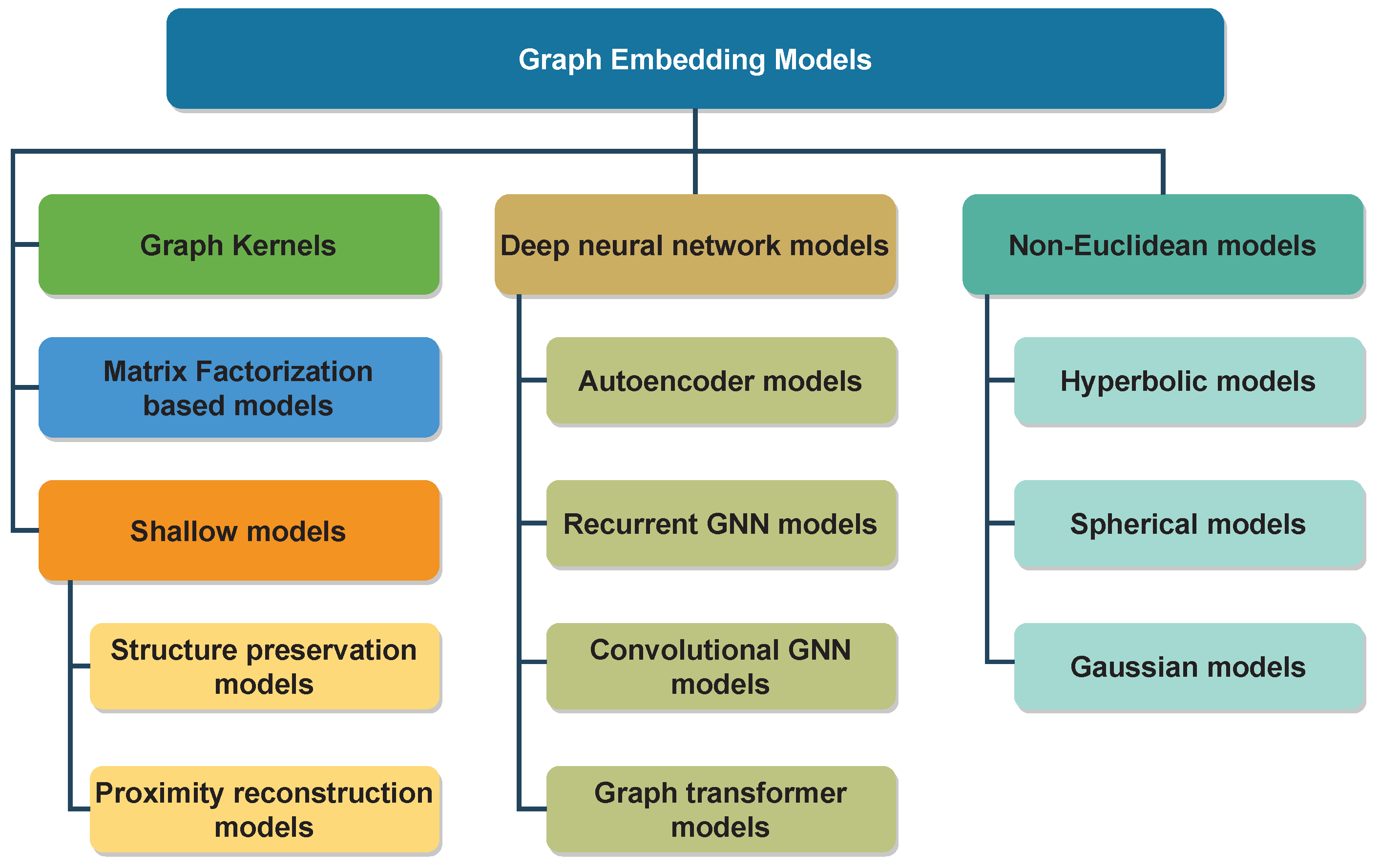
3. Graph Representation Learning Models

This section presents a taxonomy of existing graph representation learning models in the literature. We categorize the existing graph embedding models into five main groups based on strategies to preserve graph structures and proximity of entities in graphs, including graph kernels, matrix factorization-based models, shallow models, deep neural network models, and non-Euclidean models. Figure 4 presents the proposed taxonomy of the graph representation learning models. Furthermore, we deliver open-source implementations of graph embedding models in Appendix A.

Graph kernels and matrix factorization-based models are one of the pioneer models for graph representation learning. Graph kernels are prevalent in learning graph embeddings using a deterministic mapping function in solving graph classification tasks [83,84,85]. There are two types of graph kernels: kernels for graphs, which aim to compare the similarity between graphs, and kernels on graphs aim to find the similarity between nodes in graphs. Second, matrix factorization-based models aim to represent the graph as matrices and gain embeddings by decomposing the matrices [5,86]. There are several strategies for factorization modeling, and most of these models aim to approximate high-order proximity between nodes. However, graph kernels and matrix factorization-based models suffer from computational complexity when handling large graphs and capturing high-order proximity.

Shallow models aim to construct an embedding matrix to transform each graph entity into vectors. We categorize shallow models into two main groups: structure preservation and proximity reconstruction. Structure-preservation strategies aim to conserve structural relationships between nodes in graphs [4,14,87]. Depending on specific tasks, several sampling strategies could be employed to capture graph structures, such as random walks [4,14], graphlets [88], motifs [89,90,91], etc. By contrast, the objective of the proximity reconstruction models is to preserve the proximity of nodes in graphs [16,92]. The proximity strategies can vary across different models based on their objectives. For example, the LINE model [16] aims to preserve 1st-order and 2nd-order proximity between nodes, while PALE [77] preserves pairwise similarities.

Graph neural networks have shown great performance in learning complex graph structures [18,50]. GNNs can be categorized into three main groups: graph autoencoder [50,51], recurrent GNNs [17,93], and convolutional GNNs. Graph autoencoders and recurrent GNNs are mostly pioneer studies of GNNs based on autoencoder architecture and recurrent neural networks, respectively. Graph autoencoders are composed of an encoder layer and a decoder layer. The encoder layer aims to compress a proximity graph matrix to vector embeddings, and the decoder layer reconstructs the proximity matrix. Most graph autoencoder models employ multilayer perceptron-based layers or recurrent GNNs as the core of autoencoder architecture. Recurrent GNNs aim to learn node embeddings based on recurrent neural network architecture in which connections between neurons can make a cycle. Therefore, earlier RGNNs mainly aimed to learn embeddings on directed acyclic graphs [94]. Recurrent GNNs employ the same weights in all hidden layers to capture local and global structures. Recently, convolutional GNNs have been much more efficient and can gain outstanding performance compared to RGNNs. The main difference between RGNNs and CGNNs is that CGNNs use different weights in each hidden layer, which could distinguish local and global structures. Various CGNN models have been proposed and mainly fall into two categories: spectral CGNNs, and spatial CGNNs [22,52,95]. Spectral CGNNs aim to transform graph data to the frequency domain and learn node embeddings in this domain [56,96]. By contrast, spatial CGNNs work directly on the graph using convolutional filters [53,54]. By staking multiple GNN layers, the models could learn node embeddings more efficiently and capture higher-order structural information [97,98]. However, stacking many layers could cause the over-smoothing problem, which most GNNs have not fully solved in a whole extent.

Recently, several models have enabled transformer architecture to learn graph structures which gain significant results compared to other deep-learning models [30,46,99]. We categorize graph transformer models into three main groups: transformer for tree-like graphs [64,65], transformer with GNNs [99,100], and transformer with global self-attention [30,67]. Different types of graph transformer models aim to handle distinct types of graphs. The transformer for tree-like graphs aims to learn node embeddings in tree-like hierarchical graphs [64,65,101]. The hierarchical relationships from the target nodes to their parents and neighbors are presented as absolute and relative positional encoding, respectively. Several graph transformer models employ the message-passing mechanism from GNNs as an auxiliary module in computing the attention score matrix [61,100]. GNN layers can be used to aggregate information as input to graph transformer models or put on top of the model, which aims to preserve local structures. In addition, some graph transformer models can directly process graph data without support from GNN layers [30,67]. These models implement a global self-attention to learn local and global structures in a graph input without neighborhood constraints.

Most existing graph embedding models aim to learn embeddings in Euclidean space, which may not deliver good geometric representations and metrics. Recent studies have shown that non-Euclidean spaces are more suitable for representing complex graph structures. The non-Euclidean models could be categorized as hyperbolic, spherical, and Gaussian. Hyperbolic and spherical space are two types of non-Euclidean geometry that could represent different graph structures. Hyperbolic space [102] is more suitable for representing hierarchical graph structures that follow the power law, while the power of spherical space is to represent large circular graph structures [103]. Moreover, since the information about the embedding space is unknown and uncertain, several models aim at learning node embeddings as Gaussian distribution [23,104].

3.1. Graph Kernels

Graph kernels aim to compare graphs or their substructures (e.g., nodes, subgraphs, and edges) by measuring their similarity [105]. The problem of measuring the similarity of graphs is, therefore, at the core of learning graphs in an unsupervised manner. Measuring the similarity of large graphs is problematic since the graph isomorphism problem is assigned to the NP (nondeterministic polynomial time) class. However, it is an NP-complete for subgraphs isomorphism problem. Table 2 describes a summary of graph kernel models.

Kernel methods applied to the graph embedding problem can be understood in two forms, including the isomorphism testing of N graphs (kernels for graphs) and embedding entities of graphs to Hilbert space (kernels on graphs).

• Kernels for graphs: Kernels for graphs aim to measure the similarity between graphs. The similarity between the two graphs (isomorphism) could be explained as follows: Given two undirected graphs $G_1=\left(V_1{E}_1\right)$ and $G_2=\left(V_2{E}_2\right)$, $G_1$ and $G_2$ are isomorphic if they exist a bimodal mapping function $\varphi :V_1\to V_2$ such that $\forall ab\in V_1$, a and b are contiguous on $G_1$ if $\varphi \left(a\right)$ and $\varphi \left(b\right)$ are contiguous on $G_2$.
• Kernels on graphs: To embed nodes in graphs, kernel methods refer to finding a function that maps pairs of nodes to latent space using particular similarity measures. Formally, graph kernels could be defined as: Given a graph $G=(V,E)$, a function $K=V\times V\to R$ is a kernel on G if there is a mapping function $\varphi :V\to H$ such that $K\left(v_i{v}_j\right)=\langle \varphi \left(v_i\right)\varphi \left(v_j\right)\rangle$ for any node pairs $\left(v_i{v}_j\right)$.

There are several strategies to measure the similarity of pairs of graphs, such as graphlet kernels, WL kernels, random walk, and shortest paths [31,83]. Among the kernel methods, graphlet kernels are one of the simple kernels that could measure the similarity between graphs by counting subgraphs with a limited size k [83,106]. For instance, Shervashidze et al. [83] introduced a graphlet kernel with the main idea of finding the graph feature by counting the number of different graphlets in graphs. Formally, given an unlabeled graph G, a graphlet list $V_k=(G_1+G_2+\cdots +G_{n_k})$ is the set of the graphlets with size k where $n_k$ depicts the number of graphlets. The graphlet kernel for two unlabeled graphs G and $G^{\prime }$ could be defined as:

$$K\left(G,G^{\prime }\right)=\langle \varphi \left(G\right),\varphi \left(G^{\prime }\right)\rangle ,$$

(2)

where ${\varphi }^G$ and ${\varphi }^{G^{\prime }}$ are vectors that depict the number of graphlets in a $G_i$ and $G_i^{\prime }$, respectively. By counting all graphlets with size k for a graph, the computation time is expensive by the enumeration $n^k$ with n depicts the number of nodes in G. One of the practical solutions to overcome this limitation is to design the feature ${{\varphi }_i}^G$ more effectively, called Weisfeiler–Lehman.

Weisfeiler–Lehman (WL) test [31] is considered to be a traditional strategy to test the homomorphism of two graphs using color refinements. Figure 5 presents the main idea of the WL homomorphism test for two graphs in detail. By updating node labels, all the structure information of nodes in graphs could be stored at each node, including both local and global information, depending on the number of iterations. We can then compute histograms or other summary statistics over these labels as a vector representation for graphs.

Several models improved the idea from WL isomorphism test [34,84]. The concept of the WL isomorphism test inspired various GNN models later, which aim to be expressive as powerful as the WL test to distinguish different graph structures. Shervashidze et al. [33] presented three instances of WL kernels, including the WL subtree kernel, WL edge kernel, and WL shortest-path kernel with an enrichment strategy for labels. The key idea of [33] is to represent a graph G as WL sequences with the height of h. The WL sequences of two graphs G and $G^{\prime }$ can be defined as:

$$\begin{array}{cc}\hfill & k_{WL}^{\left(h\right)}\left(G,G^{\prime }\right)=k\left(G_0,G_0^{\prime }\right)+k\left(G_1,G_1^{\prime }\right)+\cdots +k\left(G_h,G_h^{\prime }\right)\hfill \end{array}$$

(3)

where $k\left(G_i,G_i^{\prime }\right)=〈\varphi \left(G_i\right),\varphi \left(G_i^{\prime }\right)〉$. For N graphs, the WL subtree kernel could be computed in a runtime of $O(Nhm+N^{2}hn)$, where h and m are the numbers of interactions and edges in G, respectively. Therefore, the algorithm could capture more information about the graph G after h interactions and compare graphs at different levels.

However, the vanilla WL isomorphism test requires massive resources since the methods are an NP-hard class. Following the WL isomorphism idea, Morris et al. [34] presented a set of k-set forms $V{\left(G\right)}_k$ and built a local and global neighborhood of the $k$-sets. Instead of working on each node in graphs, the models calculate and update the labels based on the $k$-set. The feature vectors of graph G then could be calculated by counting the number of occurrences of $k$-sets. Several models [84,114] improved the Wasserstein distance based on the WL isomorphism test, and the models could estimate weights of subtree patterns before the kernel construction [35]. Several models adopted a random-walk sampling strategy to capture the graph structure that could help reduce the computational complexity to handle large graphs [36,37,85,107].

However, the above methods only focus on homogeneous graphs in which nodes do not have side information. In the real world, graph nodes could contain labels and attributes and change over time, making it challenging to learn node embeddings. Several models have been proposed with slight variations from the traditional WL isomorphism test and random walk methods [109,110,111,112,113]. For example, Borgwardt et al. [109] presented random-walk sampling on attributed edges to capture the graph structure. Since existing kernel models primarily work on small-scale graphs or a subset of graphs, improving similarity based on shortest paths could achieve better computational efficiency for graph kernels in polynomial time. An all-paths kernel K could be defined as:

$$K\left(P\left(G_1\right),P\left(G_2\right)\right)=\sum _{p_1\in P\left(G_1\right)}\sum _{p_2\in P\left(G_2\right)}{k}_{path}\left(p_1,p_2\right),$$

(4)

where $P\left(G_1\right)$ and $P\left(G_2\right)$ are the set of random-walk paths in $G_1$ and $G_2$, respectively, and $k_{path}\left(p_1,p_2\right)$ depicts a positive definite kernel on two paths $p_1$ and $p_2$. The model then applied Floyd–Warshall algorithm [115] to find k shortest-path kernels in graphs. One of the disadvantages of this model is the runtime complexity, which is about $O(k\times n^4)$, where n depicts the number of nodes in graphs. Morris et al. [108] introduced a variation of the WL subtree kernel for attributed graphs by improving existing shortest-path kernels. The key idea of this model is to use a hash function that maps continuous attributes to label codes, and then it normalizes the discrete label codes.

To sum up, graph kernels are effective models and bring several advantages:

• Coverage: The graph kernels are one of the most useful functions to measure the similarity between graph entities by performing several strategies to find a kernel in graphs. This could be seen as a generalization of the traditional statistical methods [116].
• Efficiency: Several kernel tricks have been proposed to reduce the computational cost of kernel methods on graphs [117]. Kernel tricks could reduce the number of spatial dimensions and computational complexity on substructures while still providing efficient kernels.

Although kernel methods have several advantages, several disadvantages make the kernels difficult to scale:

• Missing entities: Most kernel models could not learn node embeddings for new nodes. In the real world, graphs are dynamic, and their entities could evolve. Therefore, the graph kernels must re-learn graphs every time a new node is added, which is time-consuming and difficult to apply in practice.
• Dealing with weights: Most graph kernel models do not consider the weighted edges, which could lead to structural information loss. This could reduce the possibility of graph representation in the hidden space.
• Computational complexity: Graph kernels are an NP-hard class [109]. Although several kernel-based models aim to reduce the computational time by considering the distribution of substructures, this may increase the complexity and reduce the ability to capture the global structure.

Although the graph kernels delivered good results when working with small graphs, they remain limitations when working with large and complex graphs [118]. To address the issue, matrix factorization-based models could bring far more advantages to learning node embeddings by decomposing the large original graphs into small-sized components. Therefore, we discuss matrix factorization-based models for learning node embeddings in the next section.

3.2. Matrix Factorization-Based Models

Matrix factorization aims to reduce the high-dimensional matrix that describes graphs (e.g., adjacency matrix, Laplacian matrix) into a low-dimensional space. Several well-known decomposition models (e.g., SVD, PCA, etc.) are widely applied in graph representation learning and recommendation system problems. Table 3 and Table 4 present matrix factorization-based models for static and dynamic graphs, respectively. Based on the strategy to preserve the graph structures, matrix factorization models could be categorized into two main groups: graph embedding Laplacian eigenmaps and node proximity matrix factorization.

• The Laplacian eigenmaps: To learn representations of a graph $G=(V,E)$, these approaches first represent G as a Laplacian matrix L where $L=D-A$ and D is the degree matrix [41]. In the matrix L, the positive values depict the degree of nodes, and negative values are the weights of the edges. The matrix L could be decomposed to find the smallest number from eigenvalues which are considered node embeddings. The optimal node embedding $Z^{*}$, therefore, could be computed using an objective function:

  $$Z^{*}=\underset{Z}{argmin}{Z}^{⊺}LZ.$$

  (5)
• Node proximity matrix factorization: The objective of these models is to decompose node proximity matrix into small-sized matrices directly. In other words, the proximity of nodes in graphs will be preserved in the latent space. Formally, given a proximity matrix M, the models try to optimize the distance between two pair nodes $v_i$ and $v_j$, which could be defined as:

  $$Z^{*}=\underset{Z}{argmin}∥M_{ij}-Z_i{Z_j}^T∥.$$

  (6)

Hofmann et al. [119] proposed an MSDC (Multidimensional Scaling and Data Clustering) model based on matrix factorization. The key idea of MSDC is to represent data points as a bipartite graph and then learn node embeddings based on node similarity in the graph. This method requires a symmetric proximity matrix $M\in {\mathbb{R}}^{N\times N}$ as input and learns a latent representation of the data in Euclidean space by minimizing the loss that could be defined as:

$$Z^{*}=\underset{Z}{argmin}\frac{1}{2\left|V\right|}{\sum _{(v_i,v_j)\in E}\left[{\left|Z_i-Z_j\right|}^2-M_{ij}\right]}^2.$$

(7)

However, the limitation of the MSDC model is that the model focuses only on the pairwise nodes, which cannot capture the global graph structure. Furthermore, the model investigated the proximity of all the data points in the graph, which could increase computational complexity when working on large graphs. Several models [39,120] adopted k-nearest methods to search neighbor nodes which can capture more graph structure. The k-nearest methods, therefore, could bring the advantage of reducing computational complexity since the models only take k neighbors as inputs. For example, Han et al. [120] proposed the similarity $S_{ij}$ between two nodes $v_i$ and $v_j$ as:

$$S_{ij}=\left\{\begin{array}{cc}exp\left(-\frac{\left|\right|v_i-v_j|{|}^2}{{\delta }^2}\right),\hfill & \mathrm{if}{v}_j\in N_k\left(v_i\right).\hfill \\ 0,\hfill & \mathrm{otherwise}.\hfill \end{array}\right.,$$

(8)

where $N_k\left(v_i\right)$ depicts the set of k nearest neighbors of $v_i$ in graphs. The model could measure the infringement of the constraints between pairs of nodes regarding label distribution. In addition, the model can estimate the correlation between features which would be beneficial to combine common features during the training process.

Several models [7,40,120,121,122] have been proposed to capture side information in graphs such as attributes and labels. He et al. [42] used the locality-preserving projection technique, a nonlinear Laplacian Eigenmap, to preserve the local structural information in graphs. The model first constructs an adjacency matrix with k nearest neighbors for each pair of nodes. The model then computes the objective function as:

$$\begin{array}{c}\hfill a^{*}=\underset{a}{argmin}{a}^{⊺}XL{X}^{⊺}a\end{array}$$

(9)

$$\begin{array}{c}\hfill \mathrm{subject}\mathrm{to}:a^{⊺}XL{X}^{⊺}a=1\end{array}$$

(10)

where D is a diagonal matrix, $L=D-A$ is the Laplacian matrix, and a is the transformation matrix in the linear embedding $x_i\to y_i=A^{⊺}{x}_i$. Nevertheless, the idea from [42] only captures the structure within k nearest neighbors, which fails to capture the global similarity between nodes in the graph. Motivated by these limitations, Cao et al. [15] introduced the GraRep model, which considers a k-hop neighborhood of each target node. Accordingly, GraRep could capture global structural information in graphs. The model works with k-order probability transition matrix (proximity matrix) $M^k$ which could be defined as:

$$M^k=\underset{k}{\underbrace{M\cdots M}}$$

(11)

where $M=D^{-1}A$, D is the degree matrix, A is the adjacent matrix, and $M_{ij}^k$ presents the transition probability from node $v_i$ to $v_j$. The loss function, thus, is the sum of k transition loss functions:

$$\begin{array}{cc}\hfill {\mathfrak{L}}_k\left(v_i\right)& =\sum _{v_j\in N\left(v_i\right)}{M}_{ij}^{k}log\sigma \left(Z_i^{⊺}{Z}_j\right)-\left|N_{neg}\right|\sum _{v_m\sim P_n\left(v\right)}{M}_{im}^{k}log\sigma \left(-Z_i^{⊺}{Z}_m\right).\hfill \end{array}$$

(12)

To construct the vector embeddings, GraRep decomposed the transition matrix into small-sized matrices using SVD matrix factorization. Similarly, Li [123] introduced NECS (Learning network embedding with the community) to capture the high-order proximity using Equation (11).

Table 3. A summary of matrix factorization-based models for static graphs. C indicates the number of clusters in graphs, $N\left(Z_i|{\mu }_c,{\Sigma }_c\right)$ refers to the multivariate Gaussian distribution for each cluster, L means the Laplacian matrix, $H\in {\mathbb{R}}^{n\times k}$ is the probability matrix that a node belongs to a cluster, U denotes the coefficient vector, and $W_{ij}$ is the weight on $(v_i,v_j)$.

Models	Graph Types	Tasks	Loss Function
SLE [39]	Static graphs	Node classification	${\sum }_{v_i\in V}{\sum }_{v_j\in V}\left|W_{ij}\right|{∥Z_i-s_{ij}{Z}_j∥}_2^2$
[120]	Attributed graphs	Node classification	$\underset{W}{argmin}Tr\left(U^{⊺}{X}^{⊺}LXU\right)+{\alpha }_{}{\sum }_{\begin{array}{c}{v}_i\in V\\ v_j\in N\left(v_i\right)\end{array}}{∥Z_i-Z_j∥}_2^2+{\alpha }_1{L}_1+{\alpha }_2{L}_2$
[7]	Attributed graphs	Community detection	$-{\displaystyle \sum _{(v_i,v_j)\in E}}log\sigma \left(Z_i^{⊺}{Z}_j\right)-{\displaystyle \sum _{\begin{array}{c}{v}_i\in V\\ v_j\in N\left(v_i\right)\end{array}}}log\sigma \left(Z_i^{⊺}{Z}_j\right)$$-\left|N_{neg}\right|{\sum }_{v_k\sim P_n\left(v\right)}log\sigma \left(-Z_i^{⊺}{Z}_k\right)-{\displaystyle \sum _{v_i\in V,c=1}^C}N\left(Z_i|{\mu }_c,{\Sigma }_c\right)$
LPP [42]	Attributed graphs	Node classification	$\frac{1}{\left|V\right|}{\sum }_{v_i\in V}{∥y_i-{\widehat{y}}_i∥}_2^2$
[121]	Attributed graphs	Graph reconstruction	$\frac{1}{\left|V\right|}{\sum }_{v_i\in V}{∥y_i-{\widehat{y}}_i∥}_2^2$
[40]	Static graphs	Node clustering	${\sum }_{v_i\in V}{\sum }_{c=1}^C∥Z_i-{\mu }_c∥$
GLEE [122]	Attributed graphs	Graph reconstruction, Link prediction	${∥L-\widehat{L}∥}^2$
LPP [42]	Static graphs	Node classification	${\sum }_{(v_i,v_j)\in E}{∥Z_i-Z_j∥}_2^2$
Grarep [15]	Static graphs	Node classification, Node clustering	$-{\sum }_{v_i\in V}{\sum }_{v_j\in N\left(v_i\right)}{A}_{ij}^{l}log\sigma \left(Z_i^{⊺}{Z}_j\right)$ $-\left|N_{neg}\right|{\sum }_{v_k~P_n\left(v\right)}{A}_{ik}^{l}log\sigma \left(\sum Z_i^{⊺}{Z}_k\right)$
NECS [123]	Static graphs	Graph reconstruction, Link prediction, Node classification	${∥M-\widehat{M}∥}_F^2+{\alpha }_1{∥H-\widehat{H}∥}_F^2+{\alpha }_2{∥H^{⊺}\widehat{H}-I∥}_F^2$
HOPE [5]	Static graphs	Graph reconstruction Link prediction, Node classification	${∥M-Z·Z^{⊺}∥}_F^2$
[124]	Static graphs	Link prediction	${\displaystyle \sum _{(v_i,v_j)\in S}}{A}_{ij}{∥Z_i-Z_j∥}_2^2$
AROPE [86]	Static graphs	Graph reconstruction, Link prediction, Node classification	${∥M-Z·Z^{⊺}∥}_F^2$
ProNE [43]	Static graphs	Node classification	$-{\sum }_{v_i\in V}\left[{\sum }_{v_j\in N\left(v_i\right)}log\sigma \left(Z_i^{⊺}{Z}_j\right)+{\displaystyle \sum _{v_k\sim P_n\left(v\right)}}log\sigma \left(-Z_i^{⊺}{Z}_k\right)\right]$
ATP [6]	Static graphs	Link prediction	${∥M-Z·Z^{⊺}∥}_F^2$
[125]	Static graphs	Graph partition	${{\displaystyle \sum _{\begin{array}{c}(v_i,v_j)\in E\\ v_i,v_j\in V_k\end{array}}}\left(W_{ij}-〈Z_i^{\left(k\right)},Z_j^{\left(k\right)}〉\right)}^2+{\displaystyle \sum _{v_i\in V_k}}{∥Z_i-{\widehat{Z}}_i∥}_2^2$
NRL-MF [126]	Static graphs	Node classification	${\displaystyle \sum _{\begin{array}{c}{v}_i\in V\\ v_j\in N\left(v_i\right)\end{array}}}{∥Z_i-Z_j∥}_2^2$

Table 3. A summary of matrix factorization-based models for static graphs. C indicates the number of clusters in graphs, $N\left(Z_i|{\mu }_c,{\Sigma }_c\right)$ refers to the multivariate Gaussian distribution for each cluster, L means the Laplacian matrix, $H\in {\mathbb{R}}^{n\times k}$ is the probability matrix that a node belongs to a cluster, U denotes the coefficient vector, and $W_{ij}$ is the weight on $(v_i,v_j)$.

Models	Graph Types	Tasks	Loss Function
SLE [39]	Static graphs	Node classification	${\sum }_{v_i\in V}{\sum }_{v_j\in V}\left|W_{ij}\right|{∥Z_i-s_{ij}{Z}_j∥}_2^2$
[120]	Attributed graphs	Node classification	$\underset{W}{argmin}Tr\left(U^{⊺}{X}^{⊺}LXU\right)+{\alpha }_{}{\sum }_{\begin{array}{c}{v}_i\in V\\ v_j\in N\left(v_i\right)\end{array}}{∥Z_i-Z_j∥}_2^2+{\alpha }_1{L}_1+{\alpha }_2{L}_2$
[7]	Attributed graphs	Community detection	$-{\displaystyle \sum _{(v_i,v_j)\in E}}log\sigma \left(Z_i^{⊺}{Z}_j\right)-{\displaystyle \sum _{\begin{array}{c}{v}_i\in V\\ v_j\in N\left(v_i\right)\end{array}}}log\sigma \left(Z_i^{⊺}{Z}_j\right)$$-\left|N_{neg}\right|{\sum }_{v_k\sim P_n\left(v\right)}log\sigma \left(-Z_i^{⊺}{Z}_k\right)-{\displaystyle \sum _{v_i\in V,c=1}^C}N\left(Z_i|{\mu }_c,{\Sigma }_c\right)$
LPP [42]	Attributed graphs	Node classification	$\frac{1}{\left|V\right|}{\sum }_{v_i\in V}{∥y_i-{\widehat{y}}_i∥}_2^2$
[121]	Attributed graphs	Graph reconstruction	$\frac{1}{\left|V\right|}{\sum }_{v_i\in V}{∥y_i-{\widehat{y}}_i∥}_2^2$
[40]	Static graphs	Node clustering	${\sum }_{v_i\in V}{\sum }_{c=1}^C∥Z_i-{\mu }_c∥$
GLEE [122]	Attributed graphs	Graph reconstruction, Link prediction	${∥L-\widehat{L}∥}^2$
LPP [42]	Static graphs	Node classification	${\sum }_{(v_i,v_j)\in E}{∥Z_i-Z_j∥}_2^2$
Grarep [15]	Static graphs	Node classification, Node clustering	$-{\sum }_{v_i\in V}{\sum }_{v_j\in N\left(v_i\right)}{A}_{ij}^{l}log\sigma \left(Z_i^{⊺}{Z}_j\right)$ $-\left|N_{neg}\right|{\sum }_{v_k~P_n\left(v\right)}{A}_{ik}^{l}log\sigma \left(\sum Z_i^{⊺}{Z}_k\right)$
NECS [123]	Static graphs	Graph reconstruction, Link prediction, Node classification	${∥M-\widehat{M}∥}_F^2+{\alpha }_1{∥H-\widehat{H}∥}_F^2+{\alpha }_2{∥H^{⊺}\widehat{H}-I∥}_F^2$
HOPE [5]	Static graphs	Graph reconstruction Link prediction, Node classification	${∥M-Z·Z^{⊺}∥}_F^2$
[124]	Static graphs	Link prediction	${\displaystyle \sum _{(v_i,v_j)\in S}}{A}_{ij}{∥Z_i-Z_j∥}_2^2$
AROPE [86]	Static graphs	Graph reconstruction, Link prediction, Node classification	${∥M-Z·Z^{⊺}∥}_F^2$
ProNE [43]	Static graphs	Node classification	$-{\sum }_{v_i\in V}\left[{\sum }_{v_j\in N\left(v_i\right)}log\sigma \left(Z_i^{⊺}{Z}_j\right)+{\displaystyle \sum _{v_k\sim P_n\left(v\right)}}log\sigma \left(-Z_i^{⊺}{Z}_k\right)\right]$
ATP [6]	Static graphs	Link prediction	${∥M-Z·Z^{⊺}∥}_F^2$
[125]	Static graphs	Graph partition	${{\displaystyle \sum _{\begin{array}{c}(v_i,v_j)\in E\\ v_i,v_j\in V_k\end{array}}}\left(W_{ij}-〈Z_i^{\left(k\right)},Z_j^{\left(k\right)}〉\right)}^2+{\displaystyle \sum _{v_i\in V_k}}{∥Z_i-{\widehat{Z}}_i∥}_2^2$
NRL-MF [126]	Static graphs	Node classification	${\displaystyle \sum _{\begin{array}{c}{v}_i\in V\\ v_j\in N\left(v_i\right)\end{array}}}{∥Z_i-Z_j∥}_2^2$

In terms of considering the node proximity based on neighbor relations, Ou et al. [5] presented HOPE, an approach for preserving structural information in graphs using k-order proximity. In contrast to GraRep, HOPE tried to solve the asymmetric transitivity problem in directed graphs by approximating high-order proximity. The objective function needs to be minimized for the approximation proximity could be defined as:

$$Z^{*}=\underset{Z}{argmin}{∥M_{ij}-Z_i^{⊺}{Z}_j∥}_2^2$$

(13)

where M is the high-order proximity matrix, for instance, $M_{ij}$ presents the proximity of two nodes $v_i$ and $v_j$, $Z_i$ and $Z_j$ denote vector embeddings of $v_i$ and $v_j$, respectively. The proximity matrix M can be measured by decomposing into two small-sized matrices $\left(M=M_g^{-1}·M_l\right)$. Several common criteria could measure the node proximity, such as Katz Index [127], Rooted PageRank [128], Adamic-Adar [129], and Common Neighbors. Coskun and Mustafa [124] suggested changes in the proximity measure formulas of the HOPE model. For nodes that have a small degree, singular values could be zero after measuring the node proximity. Therefore, to solve this problem, they added a parameter $\sigma$ to regularize the Laplacian graph.

A few models have been proposed with the same idea as HOPE and GraRep [43,86]. For example, ProNE model [43] aimed to use k number of the Chebyshev expansion to avoid Eigen decomposition, instead of using k-order proximity in HOPE models. Sun et al. [6] introduced a similar approach for preserving asymmetric transitivity with high-order proximity. However, the significant difference is that they proposed a strategy to break directed acyclic graphs while preserving the graph structure. The non-negative matrix factorization could then be applied to produce an embedding matrix. Several models [125,130,131] mainly focused on the pointwise mutual information (PMI) of nodes in graphs which calculates the connection between nodes in terms of linear and nonlinear independence. Equation (5) is used to learn node embeddings.

Several models aimed to reduce computational complexity from matrix factorization by improving the sampling strategies [126,132,133]. For instance, the key idea of the NRL-MF model [126] was to deal with a hashing function for computing dot products. Each node is presented as a binarized vector by a hashing function, which can be calculated faster by XOR operators. The model could learn the binary and quantized codes based on matrix factorization and preserve high-order proximity. Jiezhong [133] targeted sparse matrix factorization. They implemented random-walk sampling on graphs to construct a NetMF Matrix Sparsifier. RNP model [132] explored in-depth vector embeddings based on personalized PageRank values, then approximated the PPR matrices.

Table 4. A summary of matrix factorization-based models for heterogeneous graphs and dynamic graphs. $H\in {\mathbb{R}}^{n\times k}$ is the probability matrix that a node belongs to a cluster, $E^{\left(t\right)}$ is the edge matrix with type t, $W_{ij}$ is the weight on $(v_i,v_j)$, r denotes the relation type, and $E^{(1,2)}$ is the set of edges in two component graphs $G_1$ and $G_2$.

Models	Graph Types	Tasks	Loss Function
DBMM [134]	Dynamic graphs	Node classification, Node clustering	${∥A-\widehat{A}∥}_F^2$
[135]	Dynamic graphs	Link prediction	${∥A-\widehat{A}∥}_2^2+{\alpha }_{}{L}_2$
[136]	Dynamic graphs	Link prediction	${∥A-\widehat{A}∥}_F^2$
LIST [137]	Dynamic graphs	Link prediction	${∥A-\widehat{A}∥}_F^2+L_2$
TADW [131]	Attributed graphs	Node classification	${∥M-W^{⊺}HX∥}_F^2+\alpha \left({∥W∥}_F^2+{∥H∥}_F^2\right)$
PME [138]	Heterogeneous graphs	Link prediction	${\displaystyle \sum _{\begin{array}{c}(v_i,v_j)\in E^{\left(r\right)}\\ (v_i,v_k)\notin E^{\left(r\right)}\end{array}}}\left({∥Z_i-Z_j∥}_2^2-{∥Z_i-Z_{n_k}∥}_2^2+m\right)$
EOE [139]	Heterogeneous graphs	Node classification	${\displaystyle \sum _{(v_i,v_j)\in E^{(1,2)}}}\sigma \left(Z_i^{⊺}{Z}_j\right)-{\displaystyle \sum _{(v_l,v_k)\notin E^{(1,2)}}}\sigma \left(-Z_i^{⊺}{Z}_j\right)+{\alpha }_1{L}_1+{\alpha }_2{L}_2$
[130]	Heterogeneous graphs	Link prediction	${\sum }_{(v_i,v_j)\in E^{\left(t\right)}}{∥Z_i^{\left(t\right)}-{\widehat{Z}}_i^{\left(t\right)}∥}_F^2+{\alpha }_1{L}_1+{\alpha }_2{L}_2$
ASPEM [140]	Heterogeneous graphs	Node classification, Link prediction	$-{\displaystyle \sum _{\begin{array}{c}{v}_i\in V\\ (v_i,v_j,r)\in E\end{array}}}log\left(p\left(v_i\right|v_j,r)\right)$
MELL [141]	Heterogeneous graphs	Link prediction	$-{\displaystyle \sum _{(v_i,v_j)\in E}}\sigma \left(Z_i^{⊺}{Z}_j\right)-{\displaystyle \sum _{(v_i,v_k)\notin E}}\sigma \left(1-Z_i^{⊺}{Z}_k\right)+\alpha L_2$
PLE [142]	Attributed graphs	Node classification	${\sum }_{(v_i,v_j)\in E}log\sigma \left(Z_i{Z}_j\right)+\left|N_{neg}\right|E_{v_k\sim P_n\left(v_k\right)}\left(log\sigma (-Z_i{Z}_k)\right)$

Table 4. A summary of matrix factorization-based models for heterogeneous graphs and dynamic graphs. $H\in {\mathbb{R}}^{n\times k}$ is the probability matrix that a node belongs to a cluster, $E^{\left(t\right)}$ is the edge matrix with type t, $W_{ij}$ is the weight on $(v_i,v_j)$, r denotes the relation type, and $E^{(1,2)}$ is the set of edges in two component graphs $G_1$ and $G_2$.

Models	Graph Types	Tasks	Loss Function
DBMM [134]	Dynamic graphs	Node classification, Node clustering	${∥A-\widehat{A}∥}_F^2$
[135]	Dynamic graphs	Link prediction	${∥A-\widehat{A}∥}_2^2+{\alpha }_{}{L}_2$
[136]	Dynamic graphs	Link prediction	${∥A-\widehat{A}∥}_F^2$
LIST [137]	Dynamic graphs	Link prediction	${∥A-\widehat{A}∥}_F^2+L_2$
TADW [131]	Attributed graphs	Node classification	${∥M-W^{⊺}HX∥}_F^2+\alpha \left({∥W∥}_F^2+{∥H∥}_F^2\right)$
PME [138]	Heterogeneous graphs	Link prediction	${\displaystyle \sum _{\begin{array}{c}(v_i,v_j)\in E^{\left(r\right)}\\ (v_i,v_k)\notin E^{\left(r\right)}\end{array}}}\left({∥Z_i-Z_j∥}_2^2-{∥Z_i-Z_{n_k}∥}_2^2+m\right)$
EOE [139]	Heterogeneous graphs	Node classification	${\displaystyle \sum _{(v_i,v_j)\in E^{(1,2)}}}\sigma \left(Z_i^{⊺}{Z}_j\right)-{\displaystyle \sum _{(v_l,v_k)\notin E^{(1,2)}}}\sigma \left(-Z_i^{⊺}{Z}_j\right)+{\alpha }_1{L}_1+{\alpha }_2{L}_2$
[130]	Heterogeneous graphs	Link prediction	${\sum }_{(v_i,v_j)\in E^{\left(t\right)}}{∥Z_i^{\left(t\right)}-{\widehat{Z}}_i^{\left(t\right)}∥}_F^2+{\alpha }_1{L}_1+{\alpha }_2{L}_2$
ASPEM [140]	Heterogeneous graphs	Node classification, Link prediction	$-{\displaystyle \sum _{\begin{array}{c}{v}_i\in V\\ (v_i,v_j,r)\in E\end{array}}}log\left(p\left(v_i\right|v_j,r)\right)$
MELL [141]	Heterogeneous graphs	Link prediction	$-{\displaystyle \sum _{(v_i,v_j)\in E}}\sigma \left(Z_i^{⊺}{Z}_j\right)-{\displaystyle \sum _{(v_i,v_k)\notin E}}\sigma \left(1-Z_i^{⊺}{Z}_k\right)+\alpha L_2$
PLE [142]	Attributed graphs	Node classification	${\sum }_{(v_i,v_j)\in E}log\sigma \left(Z_i{Z}_j\right)+\left|N_{neg}\right|E_{v_k\sim P_n\left(v_k\right)}\left(log\sigma (-Z_i{Z}_k)\right)$

In the real world, several graphs often contain attributes for nodes and edges, such as user profiles on a social network. These attributes provide helpful information to improve the node representation and help to learn node embedding. Yang et al. [131] proposed the TADW model by representing the DeepWalk model as a matrix factorization and integrating text features into the factorization model. Ren et al. [142] introduced the PLE model to learn jointly different types of nodes and edges with text attributes. Since existing models often ignore the noise of labels, PLE is the first work to investigate the noisy type labels by measuring the similarity between entities and type labels.

Beyond static and homogeneous graphs, several models have been proposed to learn embeddings in dynamic and heterogeneous graphs. The embedding models for dynamic graphs are essentially the same as for static graphs, including Laplacian eigenmaps methods and node proximity matrix factorization to model relations in dynamic graphs over time. For Laplacian eigenmaps methods, Li et al. [81] presented DANE (Dynamic Attributed Network Embedding) model to learn node embeddings in dynamic graphs. The main idea of the DANE model is to represent a Laplacian matrix as $L_A^{\left(t\right)}=D_A^{\left(t\right)}-A^{\left(t\right)}$, where $A^{\left(t\right)}\in R^{n\times n}$ is the adjacency matrix of dynamic graphs at time t, $D_A$ is the diagonal matrix, then the model could be able to learn node embeddings by time in an online manner. To preserve the node proximity, the DANE model aimed to minimize the loss function:

$$\begin{array}{c}\hfill \mathfrak{L}(v_i,v_j)=\sum _{\begin{array}{c}(v_i,v_j)\\ i\ne j\end{array}}{A}_{ij}^{\left(t\right)}{∥Z_i-Z_j∥}_2^2.\end{array}$$

(14)

The eigenvectors $\lambda$ of the Laplacian matrix L can be calculated by solving the generalized eigenproblem: $L_A^{\left(t\right)}a=\lambda D_A^{\left(t\right)}$, where $a=\langle a_0{a}_1\cdots a_N\rangle$ is the eigenvectors.

Several models applied node proximity matrix factorization directly to dynamic graphs by updating the proximity matrix between entities in the dynamic graphs. Rossi et al. [134] presented dynamic graphs as a set of static graph snapshots: $G=\{G\left(t_0\right)G\left(t_1\right)\cdots G\left(t_N\right)\}$. The model then learned a transition proximity matrix T, which describes all transitions from the dynamic graphs. For evaluation, they predict the graph G at time $t+1$: ${\widehat{G}}_{t+1}=G_t{T}_{t+1}$, then estimate the error using Frobenius loss: ${∥{\widehat{G}}_{t+1}-G_{t+1}∥}_F$. Zhu et al. [135,137] aimed to preserve the graph structure based on temporal matrix factorization during the network evolution. Given an adjacency matrix $A\left(t\right)$ at time t, two temporal rank-k matrix factorization U and $V\left(t\right)$ are factorized as $A\left(t\right)=f\left(UV{\left(t\right)}^{⊺}\right)$, and the objective is to minimize the loss function $\mathfrak{L}\left(A\right)$ which could be defined as:

$$\begin{array}{c}\hfill \mathfrak{L}\left(A\right)=\sum _{t=1}^T\frac{D\left(t\right)}{2}{∥A\left(t\right)-\widehat{A}\left(t\right)∥}_F^2.\end{array}$$

(15)

Matrix factorization models have been successfully applied to graph embedding, mainly for the node embedding problem. Most models are based on singular value decomposition to find eigenvectors in the latent space. There are several advantages of matrix factorization-based models:

• Training data requirement: The matrix factorization-based models do not need much data to learn embeddings. Compared to other methods, such as neural network-based models, these models bring advantages in case there is little training data.
• Coverage: Since the graphs are presented as Laplacian matrix L, or transition matrix M, then the models could capture all the proximity of the nodes in the graphs. The connection of all the pairs of nodes is observed at least once time under the matrix that makes the models could be able to handle sparsity graphs.

Although matrix factorization is widely used in graph embedding problems, it still has several limitations:

• Computational complexity: The matrix factorization suffers from time complexity and memory complexity for large graphs with millions of nodes. The main reason is the time it takes to decompose the matrix into a product of small-sized matrices [15].
• Missing values: Models based on matrix factorization cannot handle incomplete graphs with unseen and missing values [143,144]. When the graph data are insufficient, the matrix factorization-based models could not learn generalized vector embeddings. Therefore, we need neural network models that can generalize graphs and better predict entities in graphs.

3.3. Shallow Models

This section focuses on shallow models for mapping graph entities into vector space. These models mainly aim to map nodes, edges, and subgraphs as low-dimensional vectors while preserving the graph structure and entity proximity. Typically, the models first implement a sampling technique to capture graph structure and proximity relation and then learn embeddings based on shallow neural network algorithms. Several sampling strategies could be taken to capture the local and global information in graphs [14,145,146]. Based on the sampling strategy, we divide shallow models into two main groups: structure preservation and proximity reconstruction.

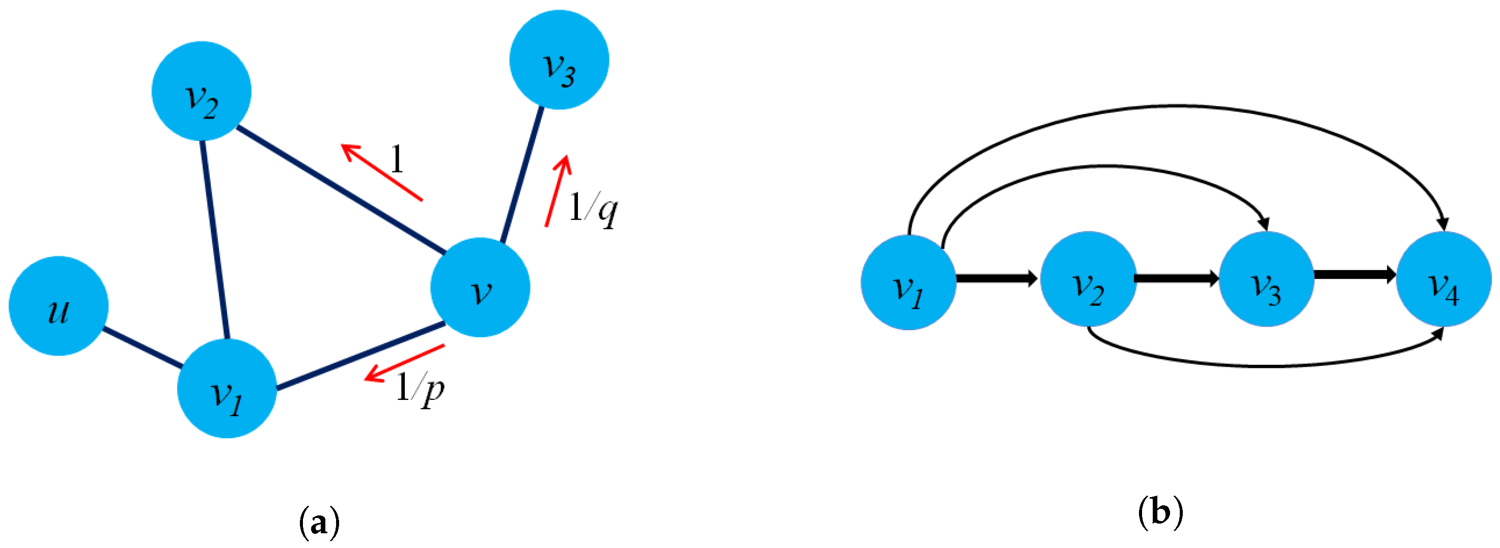
• Structure preservation: The primary concept of these approaches is to define sampling strategies that could capture the graph structure within fixed-length samples. Several sampling techniques could capture both local and global graph structures, such as random-walk sampling, role-based sampling, and edge reconstruction. The model then applies shallow neural network algorithms to learn vector embeddings in the latent space in an unsupervised learning manner. Figure 6a shows an example of a random-walk-based sampling technique in a graph from a source node $v_s$ to a target node $v_t$.
• Proximity reconstruction: It refers to preserving a k-hop relationship between nodes in graphs. The relation between neighboring nodes in the k-hop distance should be preserved in the latent space. For instance, Figure 6b presents a 3-hop proximity from the source node $v_s$.

In general, shallow models have achieved many successes in the past decade [4,14,21]. However, there are several disadvantages of shallow models:

• Unseen nodes: When there is a new node in graphs, the shallow models cannot learn embeddings for new nodes. To obtain embedding for new nodes, the models must update new patterns, for example, re-execute random-walk sampling to generate new paths for new nodes, and then the models must be re-trained to learn embeddings. The re-sampling and re-training procedures make it impractical to apply them in practice.
• Node features: Shallow models such as DeepWalk and Node2Vec mainly work suitably on homogeneous graphs and ignore information about the attributes/labels of nodes. However, in the real world, many graphs have attributes and labels that could be informative for graph representation learning. Only a few studies have investigated the attributes and labels of nodes, and edges. However, the limitations of domain knowledge when working with heterogeneous and dynamic graphs have made the model inefficient and increased the computational complexity.
• Parameter sharing: One of the problems of shallow models is that these models cannot share the parameters during the training process. From the statistical perspective, parameter sharing could reduce the computational time and the number of weight updates during the training process.

3.3.1. Structure-Preservation Models

Choosing a strategy to capture the graph structure is essential for shallow models to learn vector embeddings. The graph structure can be sampled through connections between nodes in graphs or substructures (e.g., subgraphs, motifs, graphlets, roles, etc.). Table 5 briefly summarizes structure-preservation models for static and homogeneous graphs.

Over the last decade, various models have been proposed to capture the graph structure and learn embeddings [4,21,147,148]. Among those models, random-walk-based strategies could be considered one of the most typical strategies to sample the graph structures [4,14]. The main idea of the random-walk strategy is to gather information about the graph structure to generate paths that can be treated as sentences in documents. The definition of random walks could be defined as:

Definition 6

(Random walk [14]). Given a graph $G=(V,E)$, where V is the set of nodes and E is the set of edges, a random walk with length l is a process starting at a node $v_i\in V$ and moving to its neighbors for each time step. The next steps are repeated until the length l is reached.

Two models, DeepWalk [14] and Node2Vec [4] could be considered to be pioneer models to open a new direction for learning node embeddings.

Inspired by the disadvantages of the matrix factorization-based models, the DeepWalk model could preserve the node neighborhoods based on random-walk sampling, which could capture global information in graphs. Moreover, both DeeWalk and Node2Vec aim to maximize the probability of observing node neighbors by stochastic gradient descent on each single-layer neural network. Therefore, these models reduce running time and computational complexity. DeepWalk [14] is a simple node embedding model using the random-walk sampling strategy to generate node sequences and treat them as word sentences. The objective of DeepWalk is to maximize the probability of the set of neighbor nodes $N\left(v_i\right)$ given a target node $v_i$. Formally, the optimization problem could be defined as:

$${\varphi }^{*}(·)=arg\underset{\varphi (·)}{min}-logp\left(N\left(v_i\right)|\varphi \left(v_i\right)\right)$$

(16)

where $v_i$ denotes the target node, $N\left(v_i\right)$ is the set of neighbors of $v_i$ which could be generated from random-walk sampling, $\varphi \left(v_i\right)$ is the mapping function $\varphi :v_i\in V\to R^{\left|V\right|\times d}$. The model uses two strategies for finding neighbors given a source node, based on the Breadth-First Search (BFS) and Depth First Search (DFS) strategies. The BFS strategy aims to represent a microscopic view that captures the local structure. In contrast, the DFS strategy delivers the global structure information in graphs. The DeepWalk then uses a skip-gram model and stochastic gradient descent (SGD) to learn latent representations.

Table 5. A summary of structure-preservation models for homogeneous and static graphs. K indicates the number of clusters in the graph, and ${\mu }_k$ refers to the mean value of cluster k.

Models	Graph Types	Tasks	Loss Function
DeepWalk [14]	Static graphs	Node classification	$-{\sum }_{v_i\in V}{y}_i^{⊺}log\left({\widehat{y}}_i\right)$
Node2Vec [4]	Static graphs	Node classification, Link prediction	$-{\sum }_{v_i\in V}{y}_i^{⊺}log\left({\widehat{y}}_i\right)$
WalkLets [147]	Static graphs	Node classification	$-{\sum }_{v_i\in V}{y}_i^{⊺}log\left({\widehat{y}}_i\right)$
Div2Vec [149]	Static graphs	Link prediction	$-{\sum }_{v_i\in V}{y}_i^{⊺}log\left({\widehat{y}}_i\right)$
	Static graphs	Node classification	$-{\sum }_{v_i\in V}{y}_i^{⊺}log\left({\widehat{y}}_i\right)$
Node2Vec+ [148]	Static graphs	Node classification	$-{\sum }_{v_i\in V}{y}_i^{⊺}log\left({\widehat{y}}_i\right)$
Struct2Vec [21]	Static graphs	Node classification	$-{\displaystyle \sum _{v_i\in V,〈v_i,v_j〉\in E}}log\left(\sigma \left(Z_i^{⊺}{Z}_j\right)\right)-\left|N_{neg}\right|{\displaystyle \sum _{v_k\sim P_n\left(v\right)}}log\left(\sigma (-Z_i^{⊺}{Z}_k)\right)$
DiaRW [150]	Static graphs	Node classification, Link prediction	${\sum }_{v_i\in V}-y_i^{⊺}log\left({\widehat{y}}_i\right)-(1-y_i)log(1-{\widehat{y}}_i)$
Role2Vec [151]	Attributed graphs	Link prediction	${\displaystyle \sum _{k=1}^K}{\sum }_{v_i\in V_k}{∥Z_i-{\mu }_k∥}_2^2$
NERD [152]	Directed graphs	Link Prediction, Graph Reconstruction, Node classification	${\displaystyle \sum _{(v_i,v_j)\in E}}log\sigma \left(Z_i{Z}_j\right)+\left|N_{neg}\right|E_{v_k\sim P_n\left(v_k\right)}\left(log\sigma (-Z_i{Z}_k)\right)$
Sub2Vec [153]	Static graphs	Community detection, graph classification	${\displaystyle \sum _{k=1}^K}{\sum }_{v_i\in V_k}{∥Z_i-{\mu }_k∥}_2^2$
Subgraph2Vec [145]	Static graphs	Graph classification, Clustering	$-{\sum }_{v_i\in V}{y}_i^{⊺}log\left({\widehat{y}}_i\right)$
RUM [89]	Static graphs	Node classification, Graph reconstruction	$-{\sum }_{v_i\in V}{y}_i^{⊺}log\left({\widehat{y}}_i\right)$
Gat2Vec [154]	Attributed graphs	Node classification, Link prediction	$-{\displaystyle \sum _{v_i\in V,〈v_i,v_j〉\in E}}log\left(\sigma \left(Z_i^{⊺}{Z}_j\right)\right)-\left|N_{neg}\right|{\displaystyle \sum _{v_k\sim P_n\left(v\right)}}log\left(\sigma (-Z_i^{⊺}{Z}_k)\right)$
ANRLBRW [155]	Attributed graphs	Node classification	$-{\displaystyle \sum _{v_i\in V,〈v_i,v_j〉\in E}}log\left(\sigma \left(Z_i^{⊺}{Z}_j\right)\right)-\left|N_{neg}\right|{\displaystyle \sum _{v_k\sim P_n\left(v\right)}}log\left(\sigma (-Z_i^{⊺}{Z}_k)\right)$
Gl2Vec [88]	Static graphs	Node classification	$-{\sum }_{v_i\in V}{y}_i^{⊺}log\left({\widehat{y}}_i\right)$

Table 5. A summary of structure-preservation models for homogeneous and static graphs. K indicates the number of clusters in the graph, and ${\mu }_k$ refers to the mean value of cluster k.

Models	Graph Types	Tasks	Loss Function
DeepWalk [14]	Static graphs	Node classification	$-{\sum }_{v_i\in V}{y}_i^{⊺}log\left({\widehat{y}}_i\right)$
Node2Vec [4]	Static graphs	Node classification, Link prediction	$-{\sum }_{v_i\in V}{y}_i^{⊺}log\left({\widehat{y}}_i\right)$
WalkLets [147]	Static graphs	Node classification	$-{\sum }_{v_i\in V}{y}_i^{⊺}log\left({\widehat{y}}_i\right)$
Div2Vec [149]	Static graphs	Link prediction	$-{\sum }_{v_i\in V}{y}_i^{⊺}log\left({\widehat{y}}_i\right)$
	Static graphs	Node classification	$-{\sum }_{v_i\in V}{y}_i^{⊺}log\left({\widehat{y}}_i\right)$
Node2Vec+ [148]	Static graphs	Node classification	$-{\sum }_{v_i\in V}{y}_i^{⊺}log\left({\widehat{y}}_i\right)$
Struct2Vec [21]	Static graphs	Node classification	$-{\displaystyle \sum _{v_i\in V,〈v_i,v_j〉\in E}}log\left(\sigma \left(Z_i^{⊺}{Z}_j\right)\right)-\left|N_{neg}\right|{\displaystyle \sum _{v_k\sim P_n\left(v\right)}}log\left(\sigma (-Z_i^{⊺}{Z}_k)\right)$
DiaRW [150]	Static graphs	Node classification, Link prediction	${\sum }_{v_i\in V}-y_i^{⊺}log\left({\widehat{y}}_i\right)-(1-y_i)log(1-{\widehat{y}}_i)$
Role2Vec [151]	Attributed graphs	Link prediction	${\displaystyle \sum _{k=1}^K}{\sum }_{v_i\in V_k}{∥Z_i-{\mu }_k∥}_2^2$
NERD [152]	Directed graphs	Link Prediction, Graph Reconstruction, Node classification	${\displaystyle \sum _{(v_i,v_j)\in E}}log\sigma \left(Z_i{Z}_j\right)+\left|N_{neg}\right|E_{v_k\sim P_n\left(v_k\right)}\left(log\sigma (-Z_i{Z}_k)\right)$
Sub2Vec [153]	Static graphs	Community detection, graph classification	${\displaystyle \sum _{k=1}^K}{\sum }_{v_i\in V_k}{∥Z_i-{\mu }_k∥}_2^2$
Subgraph2Vec [145]	Static graphs	Graph classification, Clustering	$-{\sum }_{v_i\in V}{y}_i^{⊺}log\left({\widehat{y}}_i\right)$
RUM [89]	Static graphs	Node classification, Graph reconstruction	$-{\sum }_{v_i\in V}{y}_i^{⊺}log\left({\widehat{y}}_i\right)$
Gat2Vec [154]	Attributed graphs	Node classification, Link prediction	$-{\displaystyle \sum _{v_i\in V,〈v_i,v_j〉\in E}}log\left(\sigma \left(Z_i^{⊺}{Z}_j\right)\right)-\left|N_{neg}\right|{\displaystyle \sum _{v_k\sim P_n\left(v\right)}}log\left(\sigma (-Z_i^{⊺}{Z}_k)\right)$
ANRLBRW [155]	Attributed graphs	Node classification	$-{\displaystyle \sum _{v_i\in V,〈v_i,v_j〉\in E}}log\left(\sigma \left(Z_i^{⊺}{Z}_j\right)\right)-\left|N_{neg}\right|{\displaystyle \sum _{v_k\sim P_n\left(v\right)}}log\left(\sigma (-Z_i^{⊺}{Z}_k)\right)$
Gl2Vec [88]	Static graphs	Node classification	$-{\sum }_{v_i\in V}{y}_i^{⊺}log\left({\widehat{y}}_i\right)$

One of the limitations of DeepWalk is that the model can only capture the graph structure but fail to navigate the random-walk sampling to enrich the quality of the sampling graph structure. To overcome the limitations of DeepWalk, Grover and Leskovec introduced Node2Vec [4] with a flexible random-walk sampling strategy to navigate random walks via each time step. The key difference between DeepWalk and Node2Vec is that instead of using a truncated random walk, the model used a biased random-walk sampling process with two parameters (p and q) to adjust the random walk on graphs. Figure 7a presents two parameters p and q in Node2Vec model in detail. The model could capture more information on the graph structure locally and globally by introducing constraints when deciding the subsequent nodes visited.

Perozzi et al. [147] presented the WalkLets model, which was extended from the DeepWalk model. They modified the random-walk sampling strategy to capture more graph structure information by skipping and passing over multiple nodes at each time step. Therefore, these sampling strategies can capture more global graph structure by the power of the transition matrix when passing over multiple nodes. The main idea of the WalkLets model is to represent the random-walk paths as pairs of nodes in the multi-scale direction. Figure 7b depicts the sampling strategy of the WalkLets model using multi-scale random-walk paths. However, one of the limitations of the WalkLets is that the model could not distinguish local and global structures when passing and skipping over nodes in graphs. Jisu et al. [149] presented a variation of DeepWalk, named Div2Vec model. The main difference between the two models is the way that Div2Vec chooses the next node in the random-walk path, which will be visited based on the degree of neighboring nodes. The focus on the degree of neighboring nodes could help the models learn the importance of nodes that are popular in social networks. Therefore, at the current node $v_i$, the probability of choosing the next node $v_j$ in a random-walk path is calculated as:

$$p\left(v_j|v_i\right)=\frac{f(deg\left(v_j\right)}{{\sum }_{v_i\in N}f(deg\left(v_i\right))}$$

(17)

where $deg\left(v_j\right)$ depicts the degree of node $v_j$, and $f(deg\left(v_j\right))=\frac{1}{deg\left(v_j\right)}$. Renming et al. [148] presented Node2Vec+, an improved version of Node2Vec. One limitation of the Node2Vec model is that it cannot determine the following nodes based on the target nodes. There is a significant difference between Node2Vec and Node2Vec+. The Node2Vec+ model can determine the state of the potential edge for a given node, therefore enhancing the navigability of the Node2Vec model to capture more graph structure. In particular, they introduced three neighboring edge states from a current node (out edge, noisy edge, and in edge) which are calculated to decide the next step. With potential out edges $(v_i,v_j)\in E$ from previous node t, the in–out parameters p and q of Node2Vec model could then be re-defined as bias factor $\alpha$ as:

$${\alpha }_{pq}(t,v_i,v_j)=\left\{\begin{array}{cc}\frac{1}{p}\hfill & \mathrm{if}t=x.\hfill \\ 1\hfill & \mathrm{if}w(v_j,t)\ge \tilde{d}\left(v_j\right).\hfill \\ min\{1,\frac{1}{p}\}\hfill & \mathrm{if}w(v_j,t)<\tilde{d}\left(v_j\right)\mathrm{and}w(v_j,t)<\tilde{d}\left(v_i\right).\hfill \\ \frac{1}{q}+(1-\frac{1}{q})\frac{w(v_j,t)}{d\left(x\right)}\hfill & \mathrm{if}w(v_j,t)<\tilde{d}\left(v_j\right)\mathrm{and}w(v_j,t)\ge \tilde{d}\left(v_i\right).\hfill \end{array}\right.$$

(18)

where $\tilde{d}\left(v_i\right)$ denotes a noisy edge threshold which could consider the next node state $v_j$ from the current node t and could be viewed as the weights of edges, $w(v_i,v_j)$ is the weight of the edge between $v_i$ and $v_j$.

In contrast to preserving graph topology which mainly focuses on distance relations, several models aimed to preserve the role and importance of nodes in graphs. In the case of social networks, for example, we could discover influencers with the ability to impact several activities of communities. In contrast to the random-walk-based technique, several studies [21,150] used the term “role-based” to preserve the nodes’ role, which random-walk-based sampling strategies cannot capture in a fixed length. Therefore, by preserving the role of nodes, role-based models could capture the structural equivalent. Ribeiro et al. [21] introduced the Struc2Vec model to capture graph structure based on the nodes’ role. Nodes that have the same degree should be encoded close in the vector space. Given a graph G, they introduced k graphs, each graph can be considered in one layer. Each layer denotes a graph that describes the weighted node degree from different hop distances. Specifically, at layer $L_k$, for each node $v_i\in V$, there are three probabilities of going to node $v_j$ in the same layer, jumping to the previous layer $L_{k-1}$ and next layer $L_{k+1}$:

$$\begin{array}{cc}\hfill p_k(v_i^k,v_j^k)& =\frac{e^{-f_k(v_i^k,v_j^k)}}{Z_k\left(v_i^k\right)}\hfill \end{array}$$

(19)

$$\begin{array}{cc}\hfill p_k(v_i^k,v_i^{k+1})& =\frac{w(v_i^k,v_i^{k+1})}{w(v_i^k,v_i^{k+1})+w(v_i^k,v_i^{k-1})}\hfill \end{array}$$

(20)

$$\begin{array}{cc}\hfill p_k(v_i^k,v_i^{k-1})& =1-p_k(v_i^k,v_i^{k+1})\hfill \end{array}$$

(21)

where $f_k\left(v_i{v}_j\right)$ presents the role-based distance between nodes $v_i$ and $v_j$, and $w(·)$ denotes the edge weight. Zhang et al. [150] presented the DiaRW model, which uses a random-walk strategy based on the node degree. The difference between other role-based models and the DiaRW model is that they used random walks that can vary in length based on the node degree. One of the limitations of the Struc2Vec model is that the model could not preserve the similarity of nodes in graphs. Motivated by this limitation, the DiaRW model aims to capture structural identity based on node degree and the neighborhood in which nodes have a high degree. The purpose of this model is to collect structural information around higher-order nodes, which is a limitation of models based on fixed-length random walks. Ahmed et al. [151] introduced the Role2Vec model that could capture the node’s similarity and structure by introducing a node-type parameter to guide random-walk paths. The core idea of Role2Vec is that nodes in the same cluster should be sampled together in the random-walk path. By only sampling nodes in the same clusters, Role2Vec could learn correct patterns with reduced computational complexity. The model then uses the skip-gram model to learn node embeddings. Unlike Rol2Vec, the NERD model [152] considers nodes’ asymmetric roles for directed graphs. The model sampled the neighbor’s nodes using an alternative random walk. The probability of the next node $v_{i+1}$ from the current node $v_i$ in the random-walk path could be defined as:

$$p\left(v_{i+1}\right|v_i)=\left\{\begin{array}{cc}\frac{1}{d^{out}\left(v_i\right)}·w(v_i,v_j)\hfill & \mathrm{if}(v_i,v_j)\in \mathrm{E}.\hfill \\ \frac{1}{d^{in}\left(v_i\right)}·w(v_i,v_j)\hfill & \mathrm{if}(v_j,v_i)\notin \mathrm{E}.\hfill \\ 0\hfill & \mathrm{otherwise}.\hfill \end{array}\right.$$

(22)

where $w(v_i,v_j)$ is the weight of the edge $e_{ij}$   $d^{in}\left(v_i\right)$ and $d^{out}\left(v_i\right)$ present the total in-degree and out-degree of the node $v_i$, respectively.

In some types of graphs, nodes in the same subgraphs tend to have similar labels. Studying low-level node representation could not bring significant generalization. Instead of embedding individual nodes in graphs, several studies aimed to learn subgraph similarity or the whole graphs. Inspired by representations of sentences and documents in the NLP (natural language processing) area, Bijaya et al. [153] proposed the Sub2Vec model to embed each subgraph into a vector embedding.

To learn a subgraph embedding $S=\{G_1{G}_2\cdots G_n\}$ from an original graph G, two properties should be preserved: similarity and structural property. The former ensures the connection between subgraph nodes by collecting sets of paths in a subgraph. The latter ensures that each node in a subgraph should be densely connected to all other nodes in the same subgraph. Figure 8 presents two subgraph properties that could capture each subgraph connection and structure.

In contrast to Sub2Vec, Subgraph2Vec [145] aimed to learn rooted subgraph embeddings for detecting Android malware. One of the advantages of this model with the Sub2Vec model is that Subgraph2Vec could consider different degrees of rooted subgraphs surrounding the target subgraph while Sub2Vec tried to detect the community. Annamalai et al. [156] targeted embedding the entire graph into the latent space. With the same idea as the Subgraph2Vec model, they extracted the set of subgraphs from the original graph using the WL relabeling strategy. However, the difference is that they used the Doc2Vec model by treating documents as graphs to learn graph embeddings.

Most models mentioned above aim to capture the graph structure based on low-level node representation, which could fail to represent the higher-level structure. Therefore, finding the community structure can be difficult for models based on random-walk sampling strategies. Motif-based models are one of the strategies to preserve the local structure and discover the global structure of graphs. Yanlei et al. [89] proposed the RUM (network Representation learning Using Motifs) model to learn small groups of nodes in graphs. The main idea of RUM was to build a new graph $G^{\prime }=(V^{\prime },E^{\prime })$ based on the original graph by constructing new nodes and edges as follows:

• Generating nodes in graph $G^{\prime }$: Each new node v in graph $G^{\prime }$ is a tuple $v_{ijk}=\langle v_i,v_j,v_k\rangle$ in the original graph G. Therefore, they can map the triangle patterns of the original graph to the new graph for structure preservation.
• Generating edges of graph $G^{\prime }$: Each edge of the new graph is formed from two nodes that have two edges in common in the original graph. For example, the edge $e=(v_{ijk},v_{ijl})$ denotes that we the edge $(v_i,v_j)\in E$ in the original graph G.

The model then used the skip-gram model to learn the node and motif embeddings. Figure 9b depicts the details of the random-walk sampling strategy based on motifs.

There are also several models based on motifs for heterogeneous graphs [87,90,91]. For instance, Qian et al. [90] proposed the MBRep model (Motif-based representation) with the same idea from the RUM model to generate a hyper-network based on a triangle motif. However, the critical difference is that the MBRep model could extract motifs based on various node and edge types in heterogeneous graphs.

Most of the above models aim to learn node embeddings without side information, which could be informative for learning graph structure. However, graphs in the real world could be composed of side information, such as attributes of nodes and edges. Several models tried to learn node embeddings in attributed graphs by adding node properties presented as attributed graphs. Nasrullah et al. [154] proposed the Gat2Vec model to capture the contextual attributes of nodes. Given by a graph $G=(V,E,X)$ where X is the attribute function $X:V\to 2^X$, they generated a structural graph $G_s$ and a bipartite graph $G_a$ as:

$$\begin{array}{cc}\hfill & G_s=\left(V_{s}E\right)\hfill \end{array}$$

(23)

$$\begin{array}{cc}\hfill & G_a=\left(V_{a}X{E}_a\right)\hfill \end{array}$$

(24)

where $V_s\subseteq V$, $V_a=\{v_i:X\left(v_i\right)\ne ⌀\}$, $V_a\subseteq V$, and $E_a=\{(v_i,a),a:X\left(v_i\right)\}$. They then used the random-walk sampling strategy to capture the graph structure in both types of graphs. Similar to Gat2Vec, Wei et al. [155] introduced the ANRLBRW model (Attributed Network Representation Learning Based on Biased Random Walk) with the idea of splitting the original graph G into a geological graph and attributed graph. However, there is a slight difference between the two models. ANRLBRW model used a biased random-walk sampling inspired by Node2Vec, which includes two parameters p and q in the sampling strategy. Kun et al. [88] introduced the Gl2Vec model to learn node embeddings based on graphlets. To generate the feature representation for graphs, they capture the proportion of graphlet occurrences in a graph compared with random graphs.

For social networks, the connections of nodes are far more complex than the node-to-node edge relationship, which constructs hypergraphs. In contrast to homogeneous graphs, edges in hypergraphs could connect more than two nodes in graphs which leads to difficult learning node embeddings. Several models have been proposed to learn node and edge embeddings in the hypergraphs [157,158]. For example, Yang et al. [157] proposed the LBSN2Vec (Location Based Social Networks) model, a hypergraph embedding model to learn hyperedges including both user-user connection and user-check-in locations over time. Since most existing models fail to capture mobility features and co-location rates dynamically, the model could learn the impact of user mobility in social networks for prediction tasks. The objective of this model is to use a random-walk-based sampling strategy on hyperedges with a sequence length to capture the hypergraph structure. They then use cousin similarity to preserve nodes’ proximity in the random-walk sequences. Table 6 lists a summary of representative models for heterogeneous graphs.

Several types of graphs in the real world are heterogeneous, with different node and edge types. Most of the above models fail to capture heterogeneous graphs. Several models have been proposed to capture the heterogeneous graph structure [159,164,166]. Dong et al. [20] introduced the Metapath2Vec model, the idea based on random walks to learn node embeddings in heterogeneous graphs. One of the powers of meta-path is that it can capture the relationship between various types of nodes and edges in heterogeneous graphs. To capture the structure of heterogeneous graphs with different types of nodes and edges, they presented meta-path random walks P with length l:

$$P:v_1\stackrel{t_1}{\to }{v}_2\stackrel{t_2}{\to }\cdots \stackrel{t_{k-1}}{\to }{v}_k\stackrel{t_k}{\to }\cdots \stackrel{t_{l-1}}{\to }{v}_l$$

(25)

where $t_i$ presents the relation type between nodes $v_i$ and $v_{i+1}$. Therefore, the transition probability of node $v_{i+1}$ given by node $v_i$ in the meta-path P could be defined as:

$$p\left(v_{i+1}\right|v_i^t,P)=\left\{\begin{array}{cc}\frac{1}{|N_{t+1}\left(v_i^t\right)|}\hfill & \mathrm{if}(v_{i+1},v_i^t)\in E{E}^{\left(t\right)}\left(v_{i+1}\right)=t+1.\hfill \\ 0,\hfill & \mathrm{otherwise}.\hfill \end{array}\right.,$$

(26)

where $N_{t+1}\left(v_i^t\right)$ is the number of the neighbors of node $v_i$ with node type $t+1$. Then, similar to DeepWalk and Node2Vec models, they used the skip-gram model to learn node embeddings. The approach from JUST [159] was conceptually similar to Metapath2Vec but the sampling strategy is performed differently. The model introduced a biased random-walk strategy with two parameters (jumping and staying) which aims to change the current domain or stay in the same domain for the next step.

Since the vanilla meta-path sampling strategy fails to capture different types of graphs, such as multiplex graphs and sparse graphs, several sampling strategies have been proposed for heterogeneous graphs based on meta-path strategies. The work of Zhang et al. [160] was similar to Metapath2Vec which implements random-walk sampling of all node types in the multiplex network. Lee et al. [161] introduced a BHIN2vec model which uses the random-walk strategy to capture sparse and rare patterns in heterogeneous graphs. Some models [162,163,164,165] have been applied to biological areas based on random-walk strategies. Lee et al. [166] used the WL relabeling strategy to capture temporal substructures of graphs. The model targeted the proximity of substructures in graphs instead of node proximity to learn the bibliographic entities in heterogeneous graphs. There are several models [167,168,176,177] that aim to capture entities from multiple networks. Du and Tong et al. [167] presented the MrMine model (Multi-resolution Multi-network) to learn embeddings with multi-resolutions. They first used WL label transformation to label nodes by the degree sequences, then adopted a dynamic time wrapping measure [21] to calculate the distance of each sequence to generate a relation network. The truncated random-walk sampling strategy is adopted to capture the graph structure. In contrast to the MrMine model, Lee and colleagues [168,176,177] explored in-depth multi-layered structure to represent the relation and proximity of individual characters, substructures, and the story network as a whole. To embed the substructure and story network, they first used WL relabeling [33] to extract substructures in the story network and then used Subgraph2Vec and Doc2Vec models to learn node embeddings.

Several types of graphs in the real world, however, show dynamic behaviors. Since most graph embedding models aim to learn node embeddings in static graphs, several models have been applied to learn node embeddings in dynamic graphs [10,92,173,174,175]. Most of them were based on the idea of DeepWalk and Node2Vec to capture the graph structure. By representing dynamic graphs as a set of static graphs, some models captured changes in the dynamic graph structure and updated changes in random walks over time. Then, the skip-gram model is used to learn node embeddings. For instance, the key idea of Sajjad et al. [169] is to generate random-walk paths on the first snapshot and then update random-walk paths in the corpus by time. Most existing models re-generate node embeddings for each graph snapshot to capture the dynamic behaviors. By contrast, the model introduced a set of dynamic random walks, which are frequently updated when there are any changes in dynamic graphs. This could reduce the computational complexity when the model handles large graphs. Figure 10 shows an example of how random-walk paths are updated in dynamic graphs.

Since the evolution of graphs only takes place at every few nodes and within a specific range of neighbors, updating the entire random walk is time-consuming. Several models [169,170,171,172,174,175] suggested updating dynamic steps over time for a few nodes and their local neighbors’ relationship. For example, Sedigheh et al. [174] presented the Dynnode2Vec model to capture the temporal evolution from graph $G_t$ to $G_{t+1}$ by a set of new nodes and edges $(V_{new},E_{new})$ and a set of removed nodes and edges $(V_{del},E_{del})$. Motivated by Node2Vec architecture, the Dynnode2Vec model could learn the dynamic structure by inducing an adequate group of random walks for only dynamic nodes. The random-walk strategy, therefore, could be more computational efficiency when the model handles large graphs. Furthermore, the proposed dynamic skip-gram model could learn node embeddings at time t by adopting the results of the previous time $t-1$ as initial weights. As a result, the dynamic skip-gram model could learn the dynamic behaviors over time.

Therefore, the changes in nodes at time $t+1$ could be described as:

$$\Delta V_t=V_{add}\cup \{v_i\in V_{t+1}|\exists e=(v_i,v_j)\in (E_{add}\cup E_{del})\}.$$

(27)

In summary, structure-preservation methods have succeeded in learning embeddings over the past decade. There are several key advantages of these models:

• Computational complexity: Unlike kernel models and matrix factorization-based models, which require considerable computational costs, structure preservation models could learn embeddings with an efficient time. This effectiveness comes from search-based sampling strategies and the model generalizability from the training process.
• Classification tasks: Since the models aim to find structural neighbor relationships from a target node, these show power in problems involving node classification. In almost all graphs, nodes that have the same label tend to be connected at a small, fixed-length distance. This is a strength of models based on preserving structure in problems related to classification tasks.

However, there are a few limitations that these models suffer when preserving the graph structure:

• Transductive learning: Most models cannot learn node embeddings that have not been seen in the training data. To learn new node embeddings, the model should re-sample the graph structure and learn the new samples again which could be time-consuming.
• Missing connection problem: Many graphs have sparse connections and missing connections between nodes in the real world. However, most structure-preservation models cannot handle missing connections between nodes since the sampling strategies could not be able to capture these connections. In the case of a random-walk-based sampling strategy, for example, these models only capture graph structure when nodes are linked together.
• Parameter sharing: These models could only learn node embeddings for individual nodes and do not share parameters. The absence of sharing parameters could reduce the effectiveness of learning representation.

3.3.2. Proximity Reconstruction Models

The purpose of graph embedding models is not only to preserve the graph structure but also to preserve the proximity of nodes in graphs. Most proximity reconstruction-based models are used for link prediction or node recommendation tasks [178,179,180] due to the nature of the similarity strategies. In this part, we discuss various models attempting to preserve the proximity of entities in graphs. Table 7 describes a summary of representative proximity reconstruction-based graph embedding models.

One of the typical models is LINE [16], which aims to preserve the symmetric proximity of node pairs in graphs. The advantage of the LINE model is that it could learn the node similarity which most structure-preservation models cannot represent this structural information. The main goal of the LINE model is to preserve the 1st-order and 2nd-order proximity of node pairs in graphs. The 1st-order proximity can be defined as follows:

Definition 7

(1st-order proximity [16]). The 1st-order proximity describes the local pairwise similarity between two nodes in graphs. Let $w_{ij}$ be the weight of an edge between two nodes $v_i$ and $v_j$, and the 1st-order proximity is defined as $w_{ij}$ when two nodes are connected and $w_{ij}=0$ when there is no link between them.

In the case of binary graphs, $w_{ij}=1$ if two nodes $v_i$ and $v_j$ are connected, and $w_{ij}=0$ otherwise. To preserve the 1st-order proximity, the objective function of two distribution ${\widehat{p}}_1(v_i,v_j)$ and $p_1(v_i,v_j)$ should be minimized:

$$\begin{array}{cc}\hfill & {\mathfrak{L}}_{\mathfrak{1}}\left(\theta \right)=\underset{\theta }{argmin}d\left({\widehat{p}}_1(v_i,v_j),p_1(v_i,v_j)|\theta \right)\hfill \end{array}$$

(28)

$$\begin{array}{cc}\hfill & {\widehat{p}}_1(v_i,v_j)=\frac{w_{ij}}{{\sum }_{(v_k,v_l)\in E}{Z}_k^{⊺}{Z}_l^{}}{p}_1(v_i,v_j)=\frac{exp\left(Z_i^{⊺}{Z}_j^{}\right)}{{\sum }_{(v_k,v_l)\in E}{Z}_k^{⊺}{Z}_l^{}}\hfill \end{array}$$

(29)

where ${\widehat{p}}_1(v_i,v_j)$ and $p_1(v_i,v_j)$ depict the empirical probability, and the actual probability of the 1st-order proximity, respectively, $v_i$ and $v_j$ are two nodes in G, $Z_i$ and $Z_j$ are embedding vectors in latent space corresponding to $v_i$ and $v_j$, respectively, $d\left(··\right)$ is the distance between the two distributions. The statistical distance, Kullback–Leibler divergence [181], is usually used to measure the difference between two distributions. In addition to preserving the proximity of two nodes that are connected directly, the LINE model also introduced 2nd-order proximity, which could be defined as follows:

Definition 8

(2nd-order proximity [16]). The 2nd-order proximity when $k=2$ captures the relationship of neighbors of each pair of nodes in the graph G. The idea of the 2nd-order proximity is that nodes should be closed if they share the same neighbors.

Let $Z_i$ and $Z_j$ are vector embeddings of nodes $v_i$ and $v_j$, respectively, the probability of the specific context $v_j$ given by the target node $v_i$ could be defined as:

$$p_2\left(v_j\right|v_i)=\frac{exp\left(Z_j^{⊺}{Z}_i\right)}{{\sum }_{v_k\in V}exp\left(Z_k^{⊺}{Z}_i\right)}.$$

(30)

Therefore, the minimization of the objective function ${\mathfrak{L}}_{\mathfrak{2}}$ could be defined as:

$${\mathfrak{L}}_{\mathfrak{2}}\left(\theta \right)=\underset{\theta }{argmin}\sum _{v_i\in V}{D}_{KL}\left({\widehat{p}}_2(.|v_i;\theta ),p_2(.|v_i)\right)$$

(31)

where ${\widehat{p}}_2\left(v_j\right|v_i)=\frac{w_{ij}}{{\sum }_{k\in N\left(i\right)}{w}_{ik}}$ is the observed distribution, $w_{ij}$ is the weighted edge between $v_i$ and $v_j$.

Table 7. A summary of proximity reconstruction models. $v_i^{\left(t\right)}$ denotes the type t of node $v_i$, $w_{ij}$ is the weight between node $v_i$ and $v_j$, P is a meta-path in heterogeneous graphs, $N_2$ is the 1st-order and 2nd-order proximity of a node $v_i$, and $P_n\left(v\right)$ is the noise distribution for negative sampling.

Models	Graph Types	Objective	Loss Function
LINE [16]	Static graphs	Node classification	$-{\displaystyle \sum _{v_i\in V,〈v_i,v_j〉\in E}}log\left(\sigma \left(Z_i^{⊺}{Z}_j\right)\right)-\left|N_{neg}\right|{\displaystyle \sum _{v_k\sim P_n\left(v\right)}}log\left(\sigma (-Z_i^{⊺}{Z}_k)\right)$
APP [76]	Static graphs	Link prediction	$-{\displaystyle \sum _{v_i\in V,〈v_i,v_j〉\in E}}log\left(\sigma \left(Z_i^{⊺}{Z}_j\right)\right)-\left|N_{neg}\right|{\displaystyle \sum _{v_k\sim P_n\left(v\right)}}log\left(\sigma (-Z_i^{⊺}{Z}_k)\right)$
PALE [77]	Static graphs	Link prediction	$-{\displaystyle \sum _{v_i\in V,〈v_i,v_j〉\in E}}log\left(\sigma \left(Z_i^{⊺}{Z}_j\right)\right)-\left|N_{neg}\right|{\displaystyle \sum _{v_k\sim P_n\left(v\right)}}log\left(\sigma (-Z_i^{⊺}{Z}_k)\right)$ ${\sum }_{〈v_i,v_j〉\in E}{∥Z_i-Z_j∥}_F^2$
CVLP [182]	Attributed graphs	Link prediction	$-{\displaystyle \sum _{\begin{array}{c}(v_i,v_j)\in E\\ (v_i,v_k)\notin E\end{array}}}log\sigma \left(Z_i^{⊺}{Z}_j-Z_i^{⊺}{Z}_k\right)+{\alpha }_1{∥Z_i-Z_j∥}_2^2+{\alpha }_2{L}_1+{\alpha }_3{L}_2$
[183]	Static graphs	Link prediction	$-{\displaystyle \sum _{〈v_i,v_j〉\in E}}{w}_{ij}log\left(p_1\left(v_i\right|v_j)\right)-{\displaystyle \sum _{〈v_i,v_j〉\in E}}{w}_{ij}log\left(p_2\left(v_j\right|v_i)\right)$
HARP [178]	Static graphs	Node classification	$-{\displaystyle \sum _{v_i\in V,〈v_i,v_j〉\in E}}log\left(\sigma \left(Z_i^{⊺}{Z}_j\right)\right)-\left|N_{neg}\right|{\displaystyle \sum _{v_k\sim P_n\left(v\right)}}log\left(\sigma (-Z_i^{⊺}{Z}_k)\right)$
PTE [179]	Heterogeneous graphs	Link prediction	$-{\sum }_{〈v_i^{\left(t\right)},v_j^{\left(t\right)}〉\in E^{\left(t\right)}}{w}_{ij}^{}log\left(v_i^{\left(t\right)}\right|v_j^{\left(t\right)})$
Hin2Vec [180]	Heterogeneous graphs	Node classification, link prediction	${\sum }_{v_i\in V}-y_i^{⊺}log\left({\widehat{y}}_i\right)-(1-y_i)log(1-{\widehat{y}}_i)$
[78]	Heterogeneous graphs	Node classification	${\sum }_{(v_i,v_j)\in E}log\sigma \left(Z_i{Z}_j\right)+\left|N_{neg}\right|E_{v_k\sim P_n\left(v_k\right)}\left(log\sigma (-Z_i{Z}_k)\right)$
[184]	Signed graphs	Link prediction	${\sum }_{v_i\in V}-y_i^{⊺}log\left({\widehat{y}}_i\right)-(1-y_i)log(1-{\widehat{y}}_i)$
[185]	Heterogeneous graphs	Node classification, Node clustering	$-{\displaystyle \sum _{(v_i,v_j)\in P}}log\left(1+e^{-Z_i{Z}_j}\right)+\left|N_{neg}\right|E_{v_k\sim P_n\left(v_k\right)}\left[log\left(1+e^{-Z_i{Z}_k}\right)\right]$
[186]	Heterogeneous graphs	Link prediction	${\displaystyle \sum _{(v_i,v_j)\in N_2}}log\sigma \left(Z_i{Z}_j\right)+\left|N_{neg}\right|E_{v_k\sim P_n\left(v_k\right)}\left(log\sigma (-Z_i{Z}_k)\right)$
[187]	Static graphs	Node classification	${\displaystyle \sum _{(v_i,v_j)\in N_2}}log\sigma \left(Z_i{Z}_j\right)+\left|N_{neg}\right|E_{v_k\sim P_n\left(v_k\right)}\left(log\sigma (-Z_i{Z}_k)\right)$
[188]	Heterogeneous graph	Graph reconstruction, link prediction, node classification	${\sum }_{v_i\in V}{∥\left(Z_i-{\widehat{Z}}_i\right)\odot B∥}_2^2+\alpha L_2$
ProbWalk [189]	Static graphs	Node classification, link prediction	${\sum }_{v_i\in V,〈v_i,v_j〉\in E}log\left(\sigma \left(Z_i^{⊺}{Z}_j\right)\right)-\left|N_{neg}\right|{\sum }_{v_k\sim P_n\left(v\right)}log\left(\sigma (-Z_i^{⊺}{Z}_k)\right)$
[190]	Static graphs	Node classification, link prediction	$\frac{1}{\left|V\right|}{\sum }_{v_i\in V}\left[y_{i}log{\widehat{y}}_i+\alpha (1-y_i)log(1-{\widehat{y}}_i)\right]$
NEWEE [191]	Static graphs	Node classification, link prediction	$-{\displaystyle \sum _{v_i\in V,〈v_i,v_j〉\in E}}log\left(\sigma \left(Z_i^{⊺}{Z}_j\right)\right)-\left|N_{neg}\right|{\displaystyle \sum _{v_k\sim P_n\left(v\right)}}log\left(\sigma (-Z_i^{⊺}{Z}_k)\right)$
DANE [192]	Attributed graphs	Node classification, Link prediction	${\displaystyle \sum _{v_i\in V}}{∥X_i-{\widehat{X}}_i∥}_2^2+{\displaystyle \sum _{v_i\in V}}{∥M_i-{\widehat{M}}_i∥}_2^2-{\displaystyle \sum _{(v_i,v_j)\in E}}log{p}_{ij}-{\displaystyle \sum _{(v_i,v_j)\in E}}\left[log{p}_{ij}-{\displaystyle \sum _{(v_i,v_j)\notin E}}log(1-p_{ij})\right]$
CENE [193]	Attributed graphs	Node classification	${\sum }_{v_i\in V}-y_i^{⊺}log\left({\widehat{y}}_i\right)-(1-y_i)log(1-{\widehat{y}}_i)$
HSCA [194]	Attributed graphs	Node classification	${∥M-W^{⊺}HX∥}_F^2+\alpha \left({∥W∥}_F^2+{∥H∥}_F^2\right)$

Table 7. A summary of proximity reconstruction models. $v_i^{\left(t\right)}$ denotes the type t of node $v_i$, $w_{ij}$ is the weight between node $v_i$ and $v_j$, P is a meta-path in heterogeneous graphs, $N_2$ is the 1st-order and 2nd-order proximity of a node $v_i$, and $P_n\left(v\right)$ is the noise distribution for negative sampling.

Models	Graph Types	Objective	Loss Function
LINE [16]	Static graphs	Node classification	$-{\displaystyle \sum _{v_i\in V,〈v_i,v_j〉\in E}}log\left(\sigma \left(Z_i^{⊺}{Z}_j\right)\right)-\left|N_{neg}\right|{\displaystyle \sum _{v_k\sim P_n\left(v\right)}}log\left(\sigma (-Z_i^{⊺}{Z}_k)\right)$
APP [76]	Static graphs	Link prediction	$-{\displaystyle \sum _{v_i\in V,〈v_i,v_j〉\in E}}log\left(\sigma \left(Z_i^{⊺}{Z}_j\right)\right)-\left|N_{neg}\right|{\displaystyle \sum _{v_k\sim P_n\left(v\right)}}log\left(\sigma (-Z_i^{⊺}{Z}_k)\right)$
PALE [77]	Static graphs	Link prediction	$-{\displaystyle \sum _{v_i\in V,〈v_i,v_j〉\in E}}log\left(\sigma \left(Z_i^{⊺}{Z}_j\right)\right)-\left|N_{neg}\right|{\displaystyle \sum _{v_k\sim P_n\left(v\right)}}log\left(\sigma (-Z_i^{⊺}{Z}_k)\right)$ ${\sum }_{〈v_i,v_j〉\in E}{∥Z_i-Z_j∥}_F^2$
CVLP [182]	Attributed graphs	Link prediction	$-{\displaystyle \sum _{\begin{array}{c}(v_i,v_j)\in E\\ (v_i,v_k)\notin E\end{array}}}log\sigma \left(Z_i^{⊺}{Z}_j-Z_i^{⊺}{Z}_k\right)+{\alpha }_1{∥Z_i-Z_j∥}_2^2+{\alpha }_2{L}_1+{\alpha }_3{L}_2$
[183]	Static graphs	Link prediction	$-{\displaystyle \sum _{〈v_i,v_j〉\in E}}{w}_{ij}log\left(p_1\left(v_i\right|v_j)\right)-{\displaystyle \sum _{〈v_i,v_j〉\in E}}{w}_{ij}log\left(p_2\left(v_j\right|v_i)\right)$
HARP [178]	Static graphs	Node classification	$-{\displaystyle \sum _{v_i\in V,〈v_i,v_j〉\in E}}log\left(\sigma \left(Z_i^{⊺}{Z}_j\right)\right)-\left|N_{neg}\right|{\displaystyle \sum _{v_k\sim P_n\left(v\right)}}log\left(\sigma (-Z_i^{⊺}{Z}_k)\right)$
PTE [179]	Heterogeneous graphs	Link prediction	$-{\sum }_{〈v_i^{\left(t\right)},v_j^{\left(t\right)}〉\in E^{\left(t\right)}}{w}_{ij}^{}log\left(v_i^{\left(t\right)}\right|v_j^{\left(t\right)})$
Hin2Vec [180]	Heterogeneous graphs	Node classification, link prediction	${\sum }_{v_i\in V}-y_i^{⊺}log\left({\widehat{y}}_i\right)-(1-y_i)log(1-{\widehat{y}}_i)$
[78]	Heterogeneous graphs	Node classification	${\sum }_{(v_i,v_j)\in E}log\sigma \left(Z_i{Z}_j\right)+\left|N_{neg}\right|E_{v_k\sim P_n\left(v_k\right)}\left(log\sigma (-Z_i{Z}_k)\right)$
[184]	Signed graphs	Link prediction	${\sum }_{v_i\in V}-y_i^{⊺}log\left({\widehat{y}}_i\right)-(1-y_i)log(1-{\widehat{y}}_i)$
[185]	Heterogeneous graphs	Node classification, Node clustering	$-{\displaystyle \sum _{(v_i,v_j)\in P}}log\left(1+e^{-Z_i{Z}_j}\right)+\left|N_{neg}\right|E_{v_k\sim P_n\left(v_k\right)}\left[log\left(1+e^{-Z_i{Z}_k}\right)\right]$
[186]	Heterogeneous graphs	Link prediction	${\displaystyle \sum _{(v_i,v_j)\in N_2}}log\sigma \left(Z_i{Z}_j\right)+\left|N_{neg}\right|E_{v_k\sim P_n\left(v_k\right)}\left(log\sigma (-Z_i{Z}_k)\right)$
[187]	Static graphs	Node classification	${\displaystyle \sum _{(v_i,v_j)\in N_2}}log\sigma \left(Z_i{Z}_j\right)+\left|N_{neg}\right|E_{v_k\sim P_n\left(v_k\right)}\left(log\sigma (-Z_i{Z}_k)\right)$
[188]	Heterogeneous graph	Graph reconstruction, link prediction, node classification	${\sum }_{v_i\in V}{∥\left(Z_i-{\widehat{Z}}_i\right)\odot B∥}_2^2+\alpha L_2$
ProbWalk [189]	Static graphs	Node classification, link prediction	${\sum }_{v_i\in V,〈v_i,v_j〉\in E}log\left(\sigma \left(Z_i^{⊺}{Z}_j\right)\right)-\left|N_{neg}\right|{\sum }_{v_k\sim P_n\left(v\right)}log\left(\sigma (-Z_i^{⊺}{Z}_k)\right)$
[190]	Static graphs	Node classification, link prediction	$\frac{1}{\left|V\right|}{\sum }_{v_i\in V}\left[y_{i}log{\widehat{y}}_i+\alpha (1-y_i)log(1-{\widehat{y}}_i)\right]$
NEWEE [191]	Static graphs	Node classification, link prediction	$-{\displaystyle \sum _{v_i\in V,〈v_i,v_j〉\in E}}log\left(\sigma \left(Z_i^{⊺}{Z}_j\right)\right)-\left|N_{neg}\right|{\displaystyle \sum _{v_k\sim P_n\left(v\right)}}log\left(\sigma (-Z_i^{⊺}{Z}_k)\right)$
DANE [192]	Attributed graphs	Node classification, Link prediction	${\displaystyle \sum _{v_i\in V}}{∥X_i-{\widehat{X}}_i∥}_2^2+{\displaystyle \sum _{v_i\in V}}{∥M_i-{\widehat{M}}_i∥}_2^2-{\displaystyle \sum _{(v_i,v_j)\in E}}log{p}_{ij}-{\displaystyle \sum _{(v_i,v_j)\in E}}\left[log{p}_{ij}-{\displaystyle \sum _{(v_i,v_j)\notin E}}log(1-p_{ij})\right]$
CENE [193]	Attributed graphs	Node classification	${\sum }_{v_i\in V}-y_i^{⊺}log\left({\widehat{y}}_i\right)-(1-y_i)log(1-{\widehat{y}}_i)$
HSCA [194]	Attributed graphs	Node classification	${∥M-W^{⊺}HX∥}_F^2+\alpha \left({∥W∥}_F^2+{∥H∥}_F^2\right)$

However, the LINE model had several limitations as it only handles symmetric proximity pairs of nodes, and the proximity of node pairs was only considered up to 2nd-order proximity. To deal with directed graphs, Chang et al. [76] introduced the APP model, which could preserve the asymmetric proximity of node pairs. They introduced two roles for each node $v_i\in V$ as the source role $s_{v_i}$ and target role $t_{v_i}$. The probability of each pair of nodes that start from a source node to the target node could be defined as:

$$p\left(v_i\right|v_j)=\frac{exp(s_{v_j}·t_{v_i})}{{\sum }_{v_k\in V}exp(s_{v_j}·t_{v_k})}.$$

(32)

Tong et al. [77] presented the PALE (Predicting Anchor Links via Embedding) model to predict the anchor links in social networks. The idea of the PALE model was the same as that of the LINE model, but they sampled only 1st-order proximity. The loss function with the negative sampling could be defined as:

$$\mathfrak{L}\left(V\right)=-\sum _{(v_i,v_j)\in E}log\sigma \left(Z_i{Z}_j\right)-\left|N_{neg}\right|E_{v_k\sim P_n\left(v_k\right)}\left(log\sigma \left(-Z_i{Z}_k\right)\right).$$

(33)

Wei et al. [182] presented the CVLP (Cross-View Link Prediction) model that could predict the connections of nodes in the context of missing and noisy attributes. Given by a triplet $(v_i,v_j,v_k)$ where $(v_i,v_j)\in E$ and $(v_i,v_k)\notin E$, the probability of proximity preservation is defined as:

$$P(s_{ij}>s_{ik}|U^g)=\sigma \left(s_{ij}-s_{ik}\right)$$

(34)

where $U^g$ is the latent representation, $s_{ij}$ is the inner product of the representation $s_{ij}=U_i^g{\left(U_j^g\right)}^{⊺}$, and $\sigma \left(·\right)$ is the sigmoid function. Li et al. [183] performed a similar study to deeply learn follower-ship and followee-ship between users across different social networks. The main idea of this model is that the proximity between nodes in a social network should be preserved in another social network. For each node $v_i$ in a graph, there are three vector representations (a node vector $Z_i$, an input context vector $Z_i^{\left(1\right)}$, and output context vector $Z_i^{\left(2\right)}$). In particular, if a node $v_i$ is following a node $v_j$ in a social network, then vector $Z_i$ should contribute to the input context of $Z_j^{\left(1\right)}$, and vector $Z_j$ should contribute to the output context of $Z_i^{\left(2\right)}$. Therefore, given a node $v_i$, the input and output context probability of node $v_j$ could be defined as follows:

$$\begin{array}{c}\hfill p_{input}\left(v_j\right|v_i)=\frac{exp\left(Z{{}_j^{\left(1\right)}}^{⊺}{Z}_i\right)}{{\sum }_{k=1}^N\left(Z{{}_k^{\left(1\right)}}^{⊺}{Z}_i\right)}{p}_{output}\left(v_i\right|v_j)=\frac{exp\left(Z{{}_j^{\left(2\right)}}^{⊺}{Z}_j\right)}{{\sum }_{k=1}^N\left(Z{{}_k^{\left(2\right)}}^{⊺}{Z}_j\right)}.\end{array}$$

(35)

Haochen et al. [178] presented HARP (Hierarchical Representation) model with a meta-strategy to capture more global proximity of each pair node in graphs. The critical difference between HARP and LINE models is that they presented the original graph G as a series of graphs $G_1,G_2,\cdots ,G_L$ where each graph can represent the collapse of adjacent edges and nodes. Figure 11 shows the way that two edges and nodes are collapsed in a graph. By representing L graphs after multiple collapses of edges and nodes, the graph can compress the proximity of nodes through supernodes.

Several variations and extensions of the LINE model are applied to heterogeneous and dynamic graphs. Jian et al. [179] presented the PTE model to preserve the 1st-order and 2nd-order proximity for heterogeneous graphs. By considering heterogeneous graphs as the set of bipartite graphs, they could independently construct the 1st-order and 2nd-order proximity for each homogeneous graph. Specifically, a bipartite graph G could be defined as $G=(V_A\cup V_B,E)$ where $V_A$ and $V_B$ are the set of nodes with different types. The probability of a node $v_i$ in the set $V_A$ given by a node $v_j$ in the set $V_B$ could be defined as follows:

$$p(v_i,v_j)=\frac{exp(Z_i^{⊺}·Z_j)}{{\sum }_{v_k\in V_A}exp(Z_k^{⊺}·Z_j)}.$$

(36)

The PTE model decomposes heterogeneous graphs into k homogeneous graphs, and the loss function is the sum of the component loss functions, which could be formulated as:

$$\begin{array}{c}\hfill \mathfrak{L}\left(V\right)=-\sum _{\left(v_i^{\left(t\right)},v_j^{\left(t\right)}\right)\in E^{\left(t\right)}}{w}_{ij}logp\left(v_i^{\left(t\right)}|v_j^{\left(t\right)}\right),\end{array}$$

(37)

where K is the number of bipartite graphs extracted from the heterogeneous graphs. Similar to the PTE model, Tao-yang et al. [180] proposed the Hin2Vec model to capture the 2nd-order proximity in heterogeneous graphs. However, instead of treating heterogeneous graphs as sets of bipartite graphs, the Hin2Vec model captured the relationship between two nodes within 2-hop distance. For instance, in the DBLP network, the relationship set is $R=\left\{P-P,P-A,A-P,P-P-P,P-P-A,P-A-P,A-P-P,A-P-A\right\}$ where P is the paper node type and A is the author node type. Zhipeng and Nikos [185] presented the HINE model (Heterogeneous Information Network Embedding) to preserve the truncated proximity of nodes. They defined an empirical joint probability of two entities in a graph as:

$$\widehat{p}(v_i,v_j)=\frac{s(v_i,v_j)}{{\sum }_{v_k\in V}s(v_i,v_k)}$$

(38)

where $v_i$ and $v_j$ are nodes, and $s(v_i,v_j)$ depicts the proximity between $v_i$ and $v_j$ in G. The proximity score $s(v_i,v_j)$ could be measured by counting the number of instances of the meta-path containing two nodes or a probability gained from implementing a random-walk sampling from $v_i$ to $v_j$.

Graphs in the real world, however, could contain attributes where several existing models, such as LINE and APP, fail to capture this information. Several models have been proposed to learn structural similarity in attributed graphs [193,195]. Sun et al. [193] proposed a CENE (content-enhanced network embedding) model to learn structural graphs and side information jointly. The objective of the CENE model is to preserve the similarity between node pairs and node-content pairs. Zhang et al. [194] proposed the HSCA (Homophily, Structure, and Content Augmented network) model to learn the homophily property of node sequences. To gain the node sequences, HSCA uses the DeepWalk model to capture the short random-walk sampling, which could represent the node context. The model then learns node embeddings based on matrix factorization by decomposing the probability transition matrix.

Most models mentioned above mainly consider the edge’s existence and ignore the dissimilarities between edges. Beyond preserving the topology and proximity of the aforementioned nodes, there are a variety of studies on edge reconstruction. The main idea of edge initialization-based models is that the edge weights can be transformed as transition probability. Wu et al. [189] introduced the ProbWalk model to learn weighted edges based on random-walk paths for edges and the skip-gram model to learn edge embeddings. The advantage of random walk on weighted edges is that this could help the model to generate more accurate node sequences and capture more useful structural information. To calculate the probability of weighted edges in graphs, they introduced a joint distribution:

$$p(v_1,v_2\cdots v_k|v_i)=\prod _{v_j\in C}\frac{e^{Z_j·Z_i}}{{\sum }_{m=1}^n{e}^{Z_m·Z_i}}$$

(39)

where $v_i$ is the target node, $C=\{v_1,v_2,\cdots ,v_k\}$ is the context of node $v_i$, and $Z_i$ is vector embedding of node $v_i$.

Alternatively, several tasks need to preserve the proximity between different relationship types of nodes. Qi et al. [190,191] proposed the NEWEE model to learn edge embeddings and then adopted a biased random-walk sampling to capture the graph structure. To learn edge embeddings, they first look for a self-centered network of each graph node. In this situation, the model could explore the similarity between edges in the self-centered network since their score tends to be higher than those in the different self-centered networks. Given a node $v_i$ in G, the self-centered network is a set of nodes containing $v_i$ and its neighbors. For example, Figure 12 depicts two self-centered networks $C_1$ and $C_2$ of node $v_1$. The objective of the model is to make all edges embedded in the same self-centered network should be close in the vector space. Therefore, given a self-centered network $G^{\prime }=(V^{\prime },E^{\prime })$, the objective function aims to maximize the proximity between edges in the same network, which could be defined as:

$$\begin{array}{c}\hfill \mathfrak{L}\left(E\right)=-\sum _{v_i\in V^{\prime }}^{}\sum _{\begin{array}{c}{e}_{ij}\in E^{\prime }\\ e_{ik}\notin E^{\prime }\end{array}}log\left[\sigma \left(e_{ij}^{⊺}{Z}_i\right)\right]+log\left[1-\sigma \left(e_{ij}^{⊺}{Z}_k\right)\right]\end{array}$$

(40)

where $e_{ij}$ denotes the edge between node $v_i$ and $v_j$ in a self-centered network $G^{\prime }$, $e_{ik}$ denotes a negative edge that $v_i$ and $v_k$ coming from different self-centered network.

In summary, compared with structure-preservation models, the proximity construction models bring several advantages:

• Inter-graph proximity: Proximity-based models not only explore proximity between nodes in a single graph but can also are applied for proximity reconstruction across different graphs with common nodes [183]. These methods can preserve the structural similarity of nodes in other graphs which are entirely different from other models. In the case of models based on structure-preservation strategies, these must re-learn node embeddings in other graphs.
• Proximity of nodes belonging to different clusters: In the context of clusters with different densities and sizes, proximity reconstruction-based models could capture nodes that are close to each other but in different clusters. This feature shows an advantage over structure reconstruction-based models, which tend to favor searching for neighboring nodes in the same cluster.
• Link prediction and node classification problem: Since structural identity is based on proximity between nodes, two nodes with similar neighborhoods should be close in the vector space. For instance, the LINE model considered preserving the 1st-order and 2nd-order proximity between two nodes. As a result, proximity reconstruction provides remarkable results for link prediction and node classification tasks [16,76,77].

However, besides the advantages of these models, there are also a few disadvantages of the proximity-based models:

• Weighted edges problems: Most proximity-based models do not consider the weighted edges between nodes. These models consider proximity based only on the number of connections shared without weights which could lead to structural loss.
• Capturing the whole graph structure: Proximity-based models mostly focus on 1st-order and 2nd-order proximity which cannot specify the global structure of graphs. A few models try to capture the higher-order proximity of nodes in graphs, but there is a problem with the computational complexity.

To overcome these limitations, shallow models should be replaced by models based on deep neural networks. Deep neural network-based models can better generalize and capture more of graph entity relationships and graph structure.

3.4. Deep Neural Network-Based Models

In recent years, large-scale graphs have challenged the ability of numerous graph embedding models. Traditional models, such as shallow neural networks or statistical methods, cannot efficiently capture complex graph structures due to their simple architecture. Recently, there have been various studies on deep graph neural networks, which are exploding rapidly because of their ability to work with complex and large graphs [11,14,23,196]. Based on the model architecture, we separate deep graph neural networks into four main groups: graph autoencoders, recurrent GNNs, convolutional GNNs, and graph transformer models. This section provides a detailed picture of deep neural network-based methods.

Unlike earlier models, most deep neural network-based models adopt the graph structure (represented as A) and node attributes/features (represented as X) to learn node embeddings. For instance, users in the social network could have text data, such as profile information. For nodes with missing attribute information, the attributes/features could be represented as node degree or one-hot vectors [72].

3.4.1. Graph Autoencoders

Graph autoencoder models are unsupervised learning algorithms that aim to encode graph entities into the latent space and reconstruct these entities from the encoded information. Based on the encoder and decoder architecture, we can classify graph autoencoder models into multilayer perceptron-based models and recurrent graph neural networks.

Early-stage graph autoencoder models are primarily based on multilayer perceptron (MLP) to learn embeddings [50,51,196]. Table 8 lists a summary of fully connected graph autoencoder models. Daixin et al. [50] introduced the SDNE model (Structural Deep Network Embedding) to capture the graph structure based on autoencoder architecture. Similar to the LINE model, the SDNE model aimed to preserve the 1st-order and 2nd-order proximity between two nodes in graphs, but it used the autoencoder-based architecture. Figure 13 presents the general architecture of the SDNE model with the corresponding encoder and decoder layers. The joint loss function that combines two loss functions for 1st-order proximity and 2nd-order proximity can be formulated as:

$$\begin{array}{cc}\hfill \mathfrak{L}\left(Z,X\right)& =\sum _{i,j=1}^n{∥(\widehat{X}-X)\odot B∥}_F^2+\lambda \sum _{i,j=1}^n{s}_{ij}{∥Z_i-Z_j∥}_2^2+L_2\hfill \end{array}$$

(41)

where $s_{ij}$ denotes the proximity between two nodes $v_i$ and $v_j$. However, the SDNE model has been proposed to learn node embeddings in homogeneous graphs. Extension of the SDNE model to heterogeneous graphs was suggested by several graph autoencoder models [51,196]. Ke et al. [51] presented the DHNE model (Deep Hyper-Network Embedding) to preserve neighborhood structures, ensuring that the nodes with similar neighborhood structures will have similar embeddings. The autoencoder layer adopts an adjacency matrix A of a hypergraph as an input, which can be formulated as:

$$A=H{H}^{⊺}-D_v$$

(42)

where $D_v$ is the diagonal matrix of node degree, and H is a matrix of size $\left|V\right|\times \left|E\right|$ presents the relation between nodes and hyperedges in graphs. The autoencoder includes two main layers: an encoder layer and a decoder layer. The encoder part takes the adjacency matrix as input and compresses it to generate node embeddings, and then the decoder part tries to reconstruct the input. Formally, the output of the encoder and decoder layer of node $v_i$ could be defined as follows:

$$\begin{array}{cc}\hfill & Z_i=\sigma (W{A}_i+b){\widehat{A}}_i=\sigma (\widehat{W}{Z}_i+\widehat{b}).\hfill \end{array}$$

(43)

One of the limitations of SDNE and DHNE models is that these models cannot handle signed graphs. Shen and Chung [197] proposed the DNE-SBP model (Deep Network Embedding with Structural Balance Preservation) to preserve the proximity of nodes in signed graphs. The DNE-SBP model constructed the input and output of the autoencoder which could be defined as:

$$\begin{array}{c}\hfill H^{\left(l\right)}=\sigma \left(X^{\left(l\right)}{\left(W_1^{\left(l\right)}\right)}^T+B_1^{\left(l\right)}\right){\widehat{X}}^{\left(l\right)}=\sigma \left({\widehat{H}}^{\left(l\right)}{\left(W_2^{\left(l\right)}\right)}^T\right)+B_2^{\left(l\right)}\end{array}$$

(44)

where $X^{\left(1\right)}=A$, $X^{\left(l\right)}=H^{(l-1)}$, and $\sigma$ is an activation function. The joint loss function is then composed of reconstruction errors with ML and CL pairwise constraints [200].

For dynamic graphs, graph autoencoder models take snapshots of graphs as inputs, and the model tries to rebuild snapshots. In several models, the output can predict future graphs by reconstructing coming snapshot graphs. Inspired by the SDNE model for static graphs, Palash et al. [198] presented the DynGEM model for dynamic graph embedding. Figure 14 presents the overview architecture of the DynGEM model. Given a sequence of graph snapshots $G=\{G_1,G_2,\cdots ,G_T\}$ and a sequence of a mapping function $\varphi =\{{\varphi }_1,{\varphi }_2,\cdots ,{\varphi }_T\}$, the DynGEM model aims to generate an embedding $Z_{t+1}={\varphi }_{t+1}\left(G_{t+1}\right)$. The stability of embeddings is the ratio of the difference between embeddings over the difference between adjacency matrices over time which could be defined as:

$$A_{abs}(\varphi ;t)=∥\frac{Z_{t+1}\left(V_t\right)-Z_t\left(V_t\right)}{A_{t+1}\left(V_t\right)-A_t\left(V_t\right)}∥$$

(45)

where $A_t$ is the weighted adjacency matrix of graph $G_t$, $Z_t\left(V_t\right)$ presents embeddings of all nodes $V_t$ at time t. The model learns parameter $\theta$ for each graph snapshot $G_t$ at time t. Similar to the SDNE model, the loss function of the DynGEM model could be defined as:

$$\mathfrak{L}(Z,X)={∥(\widehat{A}-A)\odot B∥}_F^2+\lambda \sum _{i,j=1}^n{s}_{ij}{∥Z_i-Z_j∥}_2^2+L_1+L_2$$

(46)

where $L_1$ and $L_2$ are regularization terms to prevent the over-fitting, and $s_{ij}$ is the similarity between $v_i$ and $v_j$. Similar to SDNE, Palash et al. [201] used autoencoder architecture and adopted the adjacency matrix of graph snapshots as input of the encoder layer. However, they updated parameters ${\theta }_t$ at time t based on parameter ${\theta }_{t-1}$ from the previous graph $G_{t-1}$.

Unlike the aforementioned models, Wenchao et al. [199] presented the NetWalk model that composes initial embeddings first and then updates the embeddings by learning paths in graphs, which are sampled by a reservoir sampling strategy. NetWalk model sampled the graph structure using a random-walk strategy as input to the autoencoder model. If there are any changes in dynamic graphs, the Netwalk model first updates the list of neighbors for each node and corresponding edges and then only learns embeddings again for the changes.

The aforementioned autoencoder models, which are based on feedforward neural networks, only focus on preserving pairs of nodes in graphs. Several models focus on integrating recurrent neural networks and LSTM into the autoencoder architecture, bringing prominent results, which we cover in the following section.

3.4.2. Recurrent Graph Neural Networks

One of the first models applying deep neural networks to graph representation learning was based on graph neural networks (GNNs). The main idea of GNNs is that it considers messages shared between target nodes and their neighbors until a steady balance is acquired. Table 9 summarizes graph recurrent autoencoder models.

Scarselli et al. [44,45] proposed a GNN model which could learn embeddings directly for different graphs, such as acyclic/cyclic and directed/undirected graphs. These models assumed that if nodes are directly connected in graphs, the distance between them should be minimized in the latent space. The GNN models used a data diffusion mechanism to aggregate signals from neighbor nodes (units) to target nodes. Therefore, the state of a node describes the context of its neighbors and can be used to learn embeddings. Mathematically, given a node $v_i$ in a graph, the state of $v_i$ and its output can be defined as:

$$\begin{array}{c}\hfill H_i=\sum _{v_j\in N\left(v_i\right)}{f}_w(y_i,e_{ij},H_j,y_j),Z_i=g_w(H_i,y_i),\end{array}$$

(47)

where $f_w(····)$ and $g_w(··)$ are transition functions, and $y_i$, $e_{ij}$ denote the label of node $v_i$, edge $(v_i,v_j)$, respectively. By considering the state $H_i$ that is revised by the shift process, $H_i$ and its output at layer l could be defined as:

$$\begin{array}{c}\hfill {H_i}^{\left(l\right)}=f_w\left(y_i,e_{ij},{H_j}^{(l-1)},y_j\right),{Z_i}^{\left(l\right)}=g_w\left({H_i}^{\left(l\right)},y_i\right).\end{array}$$

(48)

However, one of the limitations of GNNs is that the model learns node embeddings as single output, which could cause problems with sequence output. Several studies tried to improve GNNs using recurrent graph neural networks [17,48,49]. Unlike the GNNs which could represent a single output for each entity in a graph, Li et al. [17] attempted to output sequences by applying gated recurrent units. The model used two gated graph neural networks $F_x^{\left(l\right)}$ and $F_o^{\left(l\right)}$ to predict the output $O^l$ and the following hidden states. Therefore, the output of node $v_i$ at layer $l+1$ could be computed as:

$$\begin{array}{c}\hfill H_i^{(l+1)}=\sigma \left(H_i^{\left(l\right)},\sum _{v_j\in N\left(v_i\right)}W{H}_j^{\left(l\right)}\right),\end{array}$$

(49)

where $N\left(v_i\right)$ denotes the set of neighbors of node $v_i$.

Wang et al. [49] proposed Topo-LSTM model to capture the diffusion structure by representing graphs as a diffusion cascade to capture active and inactive nodes in graphs. Given by a cascade sequence $s=\{(v_1,1)\cdots (v_T,T)\}$, the hidden state can be represented as follows:

$$\begin{array}{cc}\hfill & h_t^{{}^{\prime }\left(p\right)}=\varphi \left(h_v\right|v\in P_v),\hfill \end{array}$$

(50)

$$\begin{array}{cc}\hfill & h_t^{{}^{\prime }\left(q\right)}=\varphi (h_v|v\in Q_v\backslash P_v),\hfill \end{array}$$

(51)

where p and q denote the input aggregation for active nodes connected with $v_t$ and not connected with the node $v_t$, respectively, $P_v$ depicts the precedent sets of active nodes at time t, and $Q_v$ depicts the set of activated nodes before time t. Figure 15 presents an example of the Topo-LSTM model. However, these models could not capture global graph structure since they only capture the graph structure within k-hop distance. Several models have been proposed by combining graph recurrent neural network architecture with random-walk sampling structure to capture higher structural information [48,93]. Huang et al. [93] introduced the GraphRNA model to combine a joint random-walk strategy on attributed graphs with recurrent graph networks. One of the powers of the random-walk sampling strategy is to capture the global structure. By considering the node attributes as a bipartite network, the model could perform joint random walks on the bipartite matrix containing attributes to capture the global structure of graphs. After sampling the node attributes and graph structure through joint random walks, the model uses graph recurrent neural networks to learn embeddings. Similar to GraphRNA model, Zhang et al. [48] presented the SHNE model to analyze the attributes’ semantics and global structure in attributed graphs. The SHNE model also used a random-walk strategy to capture the global structure of graphs. However, the main difference between SHNE and GraphRNA is that the SHNE model first applied GRU (gated recurrent units) model to learn the attributes and then combined them with graph structure via random-walk sampling.

Since the power of autoencoders architecture is to learn compressed representations, several studies [57,205] aimed to combine RGNNs and autoencoders with learning node embeddings in weighted graphs. For instance, Seo and Lee [57] adopted an LSTM autoencoder to learn node embeddings for weighted graphs. They used the BFS algorithm to travel nodes in graphs and extract the node-weight sequences of graphs as inputs for the LSTM autoencoder. The model then could leverage the graph structure reconstruction based on autoencoder architecture and the node attributes by the LSTM model. Figure 16 presents the sampling strategy of this model, which lists the nodes and their respective weighted edges. To capture local and global graph structure, Aynaz et al. [205] proposed a sequence-to-sequence autoencoder model, which could represent inputs with arbitrary lengths. The LSTM-based autoencoder model architecture consists of two main parts: The encoder layer ${LSTM}_{enc}$ and the decoder layer ${LSTM}_{dec}$. For the sequence-to-sequence autoencoder, at each time step l, the hidden vectors in the encoder and decoder layers can be defined as:

$$\begin{array}{c}\hfill h_{enc}^t={LSTM}_{enc}\left(Z_i^{\left(t\right)},h_{enc}^{t-1}\right),h_{dec}^t={LSTM}_{dec}\left(Z_i^{(t-1)},h_{dec}^{t-1}\right)\end{array}$$

(52)

where $h_{enc}^t$ and $h_{dec}^t$ are the hidden states at step t in the encoder and decoder layers, respectively. To generate the sequences of nodes, the model implemented different sampling strategies, including random walks, shortest paths, and breadth-first search with the WL algorithm to encode the information of node labels.

Since the aforementioned models learn node embeddings for static graphs, Shima et al. [203] presented an LSTM-Node2Vec model by combining an LSTM-based autoencoder architecture with the Node2Vec model with learning embeddings for dynamic graphs. The idea of the LSTM-Node2Vec model is that it uses an LSTM autoencoder to preserve the history of node evolution with a temporal random-walk sampling. It then adopted the Node2Vec model to generate the vector embeddings for the new graphs. Figure 17 presents a temporal random-walk sampling strategy to travel a dynamic graph.

Jinyin et al. [204] presented the E-LSTM-D model (Encoder-LSTM-Decoder) to learn embeddings for dynamic graphs by combining autoencoder architecture and LSTM layers. Given by a set of graph snapshots $S=\{G_{t-k},G_{t-k+1},\cdots ,G_{t-1}\}$, the objective of the model is to learn a mapping function $\varphi :\varphi \left(S\right)\to G_t$. The model takes the adjacency matrix as the input of the autoencoder model, and the output of the encoder layer could be defined as:

$$\begin{array}{ccc}\hfill H_{e,i}^{\left(1\right)}& =& ReLU\left(W_e^{\left(1\right)}{\mathrm{s}}_i^{}+b_i^{\left(1\right)}\right)\hfill \end{array}$$

(53)

$$\begin{array}{ccc}\hfill H_{e,i}^{\left(l\right)}& =& ReLU\left(W_e^{\left(l\right)}{b}_{e,i}^{(l-1)}+b_e^{\left(l\right)}\right)\hfill \end{array}$$

(54)

$$\begin{array}{ccc}\hfill H_e^{\left(l\right)}& =& \left[H_{e,0}^{\left(l\right)},H_{e,1}^{\left(l\right)},\cdots ,H_{e,N-1}^{\left(l\right)}\right]\hfill \end{array}$$

(55)

where $s_i$ denotes the i-th graph in the series of graph snapshots, $\mathrm{ReLU}(·)=max(0,·)$ is the activation function. For the decoder layer, the model tried to reconstruct the original adjacency matrix from vector embeddings, which could be defined as follows:

$$\begin{array}{ccc}\hfill H_d^{\left(1\right)}& =& ReLU\left(W_d^{\left(1\right)}{H}_e+b_d^{\left(1\right)}\right)\hfill \end{array}$$

(56)

$$\begin{array}{ccc}\hfill H_d^{\left(l\right)}& =& ReLU\left(W_d^{\left(l\right)}{H}_d^{(l-1)}+b_d^{\left(l\right)}\right)\hfill \end{array}$$

(57)

where $H_e$ depicts the output of the stacked LSTM model, which captures the current graph’s structure $G_t$. Similar to E-LSTM-D model, Palash et al. [201] proposed a variant of Dyngraph2Vec model, named Dyngraph2VecAERNN (Dynamic Graph to Vector Autoencoder Recurrent Neural Network) which also considers the adjacency matrix as input for the model. However, the critical difference between the E-LSTM-D model and the Dyngraph2VecAERNN model is that they feed the LSTM layers directly into the encoder part to learn embeddings. The decoder layer is composed of fully connected neural network layers to reconstruct the inputs.

There are several advantages of recurrent graph neural networks compared to shallow learning techniques:

• Diffusion pattern and multiple relations: RGNNs show superior learning ability when dealing with diffuse information, and they can handle multi-relational graphs where a single node has many relations. This feature is achieved due to the ability to update the states of each node in each hidden layer.
• Parameter sharing: RGNNs could share parameters across different locations, which could be able to capture the sequence node inputs. This advantage could reduce computational complexity during the training process with fewer parameters and increase the performance of the models.

However, one of the disadvantages of the RGNNs is that these models use recurrent layers with the same weights during the weight update process. This leads to inefficiencies in representing different relationship constraints between neighbor and target nodes. To overcome the limitation of RGNNs, convolutional GNNs have shown remarkable ability in recent years when it uses different weights in each hidden layer.

3.4.3. Convolutional Graph Neural Networks

CNNs have achieved remarkable success in the image processing area. Since image data can be considered to be a special case of graph data, convolution operators can be defined and applied to graph mining. There are two strategies to implement when applying convolution operators to the graph domain. The first strategy is based on graph spectrum theory which transforms graph entities from the spatial domain to the spectral domain and applies convolution filters on the spectral domain. The other strategy directly employs the convolution operators in the graph domain (spatial domain). Table 10 summarizes spectral CGNN models.

When computing power is insufficient for implementing convolution operators directly on the graph domain, several studies focus on transforming graph data to the spectral domain and applying filtering operators to reduce computational time [18,55,213]. The signal filtering process acts as the feature extraction on the Laplacian matrix. Most models adopted single and undirected graphs and presented graph data as a Laplacian matrix:

$$\begin{array}{c}\hfill L=I_n-D^{-\frac{1}{2}}A{D}^{-\frac{1}{2}}\end{array}$$

(58)

where D denotes the diagonal matrix of the node degree, A is the adjacency matrix. The matrix L is a symmetric positive definite matrix describing the graph structure. Considering a matrix U as a graph Fourier basis, the Laplacian matrix then could be decomposed into three components: $L=U\Lambda U^{⊺}$ where $\Lambda$ is the diagonal matrix which denotes the spectral representation of graph topology and $U=[u_0,u_1,\cdots ,u_{n-1}]$ is eigenvectors matrix. The filter function $g_{\theta }$ resembles a k-order polynomial, and the spectral convolution acts as diffusion convolution in graph domains. The spectral graph convolution given by an input x with a filter $g_{\theta }$ is defined as:

$$\begin{array}{c}\hfill g_{\theta }\ast x=U_{g_{\theta }}{U}^{⊺}x\end{array}$$

(59)

where ∗ is the convolution operation. Bruna et al. [56] transformed the graph data to the spectral domain and applied filter operators on a Fourier basis. The hidden state at the layer l could be defined as:

$$\begin{array}{c}\hfill H_i^{\left(l\right)}=\sigma \left(V\sum _{j=1}^{c_{l-1}}{D}_{ij}^{\left(l\right)}{V}^{⊺}{H}_j^{\left(l\right)}\right)\end{array}$$

(60)

where $D_{ij}^{\left(l\right)}$ is a diagonal matrix at layer l, $c_{l-1}$ denotes the number of filters at layer $l-1$, and V denotes the eigenvectors of the L matrix. Typically, most of the energy of the D matrix is concentrated in the first d elements. Therefore, we can obtain the first d values of the matrix V, and the number of parameters that should be trained is $c_{l-1}·c_l·d$.

Several studies focused on improving spectral filters to reduce computational time and capture more graph structure in the spectral domain [210,216]. For instance, Defferrard et al. [216] presented a strategy to re-design convolutional filters for graphs. Since the spectral filter $g_{\theta }(\Lambda )$ indeed generates a kernel on graphs, the key idea is that they consider $g_{\theta }(\Lambda )$ as a polynomial which includes k-localized kernel:

$$\begin{array}{c}\hfill g_{\theta }(\Lambda )=\sum _{k=0}^{K-1}{\theta }_k{\Lambda }^{\left(k\right)}\end{array}$$

(61)

where $\theta$ is a vector of polynomial coefficients. This k-localized kernel provides a circular distribution of weights in the kernel from a target node to k-hop nodes in graphs.

Unlike the above models, Zhuang and Ma [211] tried to capture the local and global graph structures by introducing two convolutional filters. The first convolutional operator, local consistency convolution, captures the local graph structure. The output of a hidden layer $Z^l$, then, could be defined as:

$$\begin{array}{c}\hfill Z^{\left(l\right)}=\sigma \left({\tilde{D}}^{-\frac{1}{2}}\tilde{A}{\tilde{D}}^{-\frac{1}{2}}{Z}^{(l-1)}{W}^{\left(l\right)}\right)\end{array}$$

(62)

where $\tilde{A}=A+I$ denotes the self-loops adjacency matrix, and ${\tilde{D}}_{i.i}={\sum }_j{\tilde{A}}_{ij}$ is the diagonal matrix presenting the degree information of nodes. In addition to the first filter, the second filter aims to capture the global structure of graphs which could be defined as:

$$\begin{array}{c}\hfill Z^{\left(l\right)}=\sigma \left(D^{-\frac{1}{2}}AP{D}^{-\frac{1}{2}}{Z}^{(l-1)}{W}^{\left(l\right)}\right)\end{array}$$

(63)

where P denotes the PPMI matrix, which can be calculated via frequency matrix using random-walk sampling.

Most of the above models learn node embeddings by transforming graph data to signal domain and use convolutional filters which lead to increased computational complexity. In 2016, Kipf and Welling [18] introduced graph convolutional networks (GCNs), which were considered to be a bridge between spectral and spatial approaches. The spectral filter $g_{\theta }(\Lambda )$ and the hidden layers of the GCN model followed the layer-wise propagation rule can be defined as follows:

$$\begin{array}{cc}\hfill & g_{{\theta }^{\prime }}(\Lambda )\approx \sum _{k=0}^K{{\theta }^{\prime }}_k{T}_k\left(\tilde{\Lambda }\right)\hfill \end{array}$$

(64)

$$\begin{array}{cc}\hfill & H^{(l+1)}=\sigma \left({\tilde{D}}^{-\frac{1}{2}}A{\tilde{D}}^{-\frac{1}{2}}{H}^{\left(l\right)}{W}^{\left(l\right)}\right)\hfill \end{array}$$

(65)

where $\tilde{\Lambda }=\frac{2}{{\lambda }_{max}}\Lambda -I_N$ and ${\lambda }_{max}$ is the largest eigenvalue of Laplacian matrix L, ${\theta }^{\prime }\in {\mathbb{R}}^K$ is Chebyshev coefficients vector, $T_k\left(x\right)$ is Chebyshev polynomials could be defined as:

$$\begin{array}{cc}\hfill & T_k\left(x\right)=2x{T}_{k-1}\left(x\right)-T_{k-2}\left(x\right)\hfill \end{array}$$

(66)

where $T_0\left(x\right)=1\mathrm{and}{T}_1\left(x\right)=x$. Consequently, the convolution filter of an input x is defined as:

$$\begin{array}{c}\hfill g_{{\theta }^{\prime }}\ast x\approx \sum _{k=0}^K{{\theta }^{\prime }}_k{T}_k\left(\tilde{L}\right)x,\tilde{L}=\frac{2}{{\lambda }_{max}}L-I_N.\end{array}$$

(67)

Although spectral CGNNs are effective in applying convolution filters on the spectral domain, they have several limitations as follows:

• Computational complexity: The spectral decomposition of the Laplacian matrix into matrices containing eigenvectors is time-consuming. During the training process, the dot product of the U, $\Lambda$, and $U^T$ matrices also increase the training time.
• Difficulties for handling large-scale graphs: Since the number of parameters for the kernels also corresponds to the number of nodes in graphs. Therefore, spectral models could not be suitable for large-scale graphs.
• Difficulties for considering graph dynamicity: To apply convolution filters to graphs and train the model, the graph data must be transformed to the spectral domain in the form of a Laplacian matrix. Therefore, when the graph data changes, in the case of dynamic graphs, the model is not applicable to capture changes in dynamic graphs.

Motivated by the limitations of spectral domain-based CGNNs, spatial models apply convolution operators directly to the graph domain and learn node embeddings in an effective way. Recently, various spatial CGNNs have been proposed showing remarkable results in handling different graph structures compared to spectral models [52,95]. Based on the mechanism of aggregation from graphs and how to apply the convolution operators, we divide CGNN models into the following main groups: (i) Aggregation mechanism improvement, (ii) Training efficiency improvement, (iii) Attention-based models, and (iv) Autoencoder-CGNN models. Table 11 and Table 12 present a summary of spatial CGNN models for all types of graphs ranging from homogeneous to heterogeneous graphs.

Gilmer et al. [222] presented the MPNN (Message-Passing Neural Network) model to employ the concept of messages passing over nodes in graphs. Given a pair of nodes $(v_i,v_j)$, a message from $v_j$ to $v_i$ could be calculated by a message function $M_{ij}$. During the message-passing phase, a hidden state at layer l of a node $v_i$ could be calculated based on the message-passing from its neighbors, which could be defined as:

$$\begin{array}{cc}\hfill & m_i^{(l+1)}=\sum _{v_j\in N\left(v_i\right)}{M}_{\left(l\right)}\left(h_i^{\left(l\right)},h_j^{\left(l\right)},e_{ij}\right),\hfill \end{array}$$

(68)

$$\begin{array}{cc}\hfill & h_i^{(l+1)}=\sigma \left(h_i^{\left(l\right)},m_i^{(l+1)}\right),\hfill \end{array}$$

(69)

where $M_{\left(l\right)}$ denotes the message function at layer l which could be a MLP function, $\sigma$ is an activation function, and $N\left(v_i\right)$ denotes the set of neighbors of node $v_i$.

Most previous graph embedding models work in transductive learning which cannot handle unseen nodes. In 2017, Hamilton et al. [22] introduced the GraphSAGE model (SAmple and aggreGatE) to generate inductive node embeddings in an unsupervised manner. The hidden state at layer $l+1$ of a node $v_i$ could be defined as:

$$\begin{array}{c}\hfill h_i^{(l+1)}={AGG}_{(l+1)}\left(\{h_j^{\left(l\right)},\forall v_j\in N\left(v_i\right)\}\right)\end{array}$$

(70)

where $N\left(v_i\right)$ denotes the set of neighbors of node $v_i$, $h_j^{\left(l\right)}$ is the hidden state of node $v_j$ at layer l. The function $AGG(··)$ is a differentiable aggregator function. There are three aggregators (e.g., Mean, LSTM, and Pooling) to aggregate information from neighboring nodes and separate nodes into mini batches. Algorithm 1 presents the algorithm of the GraphSAGE model.

Algorithm 1: GraphSAGE algorithm. The model first takes the node features as inputs. For each layer, the model aggregates the information from neighbors and then updates the hidden state of each node $v_i$.

Input: $G=(V,E)$: The graph G with set of nodes V and set of edges E.             $x_i$: The input features of node $v_i$             L: The depth of hidden layers, $\forall l\in \{1\cdots L\}$             ${AGG}_k$: Differentiable aggregator functions             $N\left(v_i\right)$: The set of neighbors of node $v_i$. Output: $Z_i$: Vector representations for $v_i$. $h_i^0\leftarrow x_i,\forall v_i\in V$ $Z_i\leftarrow h_i^L,\forall v_i\in V$

Lo et al. [231] aimed to apply the GraphSAGE model to detect computer attackers in computer network systems, named E-graphSAGE. The main difference between the two models is that E-graphSAGE used the edges of graphs as aggregation information for learning embeddings. The edge information between two nodes is the data flow between two source IP addresses (Clients) and destination IP addresses (Servers).

By evaluating the contribution of neighboring nodes to target nodes, Tran et al. [229] proposed convolutional filters with different parameters. The key idea of this model is to rank the contributions of different distances from the set of neighbor nodes to target nodes using short path sampling. Formally, the hidden state of a node at layer $l+1$ could be defined as multiple graph convolutional filters:

$$\begin{array}{c}\hfill h^{r,l+1}{=\Vert }_{j=0}^r\left({\left(D^j\right)}^{-1}S{P}^j{h}^l{W}^{j,l}\right)\end{array}$$

(71)

where ‖ denotes the concatenation, r and $S{P}^j$ denote the r-hop distance and the shortest-path distance j, respectively. Ying et al. [225] considered random-walk sampling as the aggregation information that can be aggregated to the hidden state of CGNNs. To collect the neighbors of node v, the idea of the model is to gather a set consisting of random-walk paths from node v and then select the top k nodes with the highest probability.

For hypergraphs, several GNN models have been proposed to learn high-order graph structure [27,44,234]. Feng et al. [27] proposed HGNN (Hypergraph Neural Networks) model to learn hypergraph structure based on spectral convolution. They first learn each hyperedge feature by aggregating all the nodes connected by the hyperedge. Then, each node’s attribute is updated with a vector embedding based on all the hyperedges connecting to the nodes. By contrast, Yadati [234] presented the HyperGCN model to learn hypergraphs based on spectral theory. Since each hyperedge could connect several nodes between them, this model’s idea is to filter far apart nodes. Therefore, they adopt the Laplacian operator first to learn node embedding and filter edges, which connect two nodes at a high distance. The GCNs could then be used to learn node embeddings.

One of the limitations of GNN models is that the models consider the set of neighbors as permutation invariant. This limitation then makes the models cannot distinguish between isomorphic subgraphs. By considering the message-passing set from neighbors of nodes as permutation invariant, several works aimed to improve the message-passing mechanism by simple aggregation functions. Xu et al. [24] proposed GIN (Graph Isomorphism Network) model, which aims to learn vector embeddings as powerful as the 1-dimensional WL isomorphism test. Formally, the hidden state of node $v_i$ at layer l could be defined as:

$$\begin{array}{c}\hfill h_i^{\left(l\right)}={MLP}^{\left(l\right)}\left(\left(1+{\epsilon }^{\left(l\right)}\right)·h_i^{(l-1)}+{\sum }_{v_j\in N\left(v_i\right)}{h}_j^{(l-1)}\right)\end{array}$$

(72)

where MLP denotes multilayer perceptions and $\epsilon$ is a parameter that could be learnable or fixed scalar. Another problem of GNNs is the over-smoothing problem when stacking more layers in the models. DeeperGCN [98] was a similar approach that aims to solve the over-smoothing problem by generalized aggregations and skip connections. The DeeperGCN model defined a simple normalized message-passing, which could be defined as:

$$\begin{array}{cc}\hfill & m_{ij}^{\left(l\right)}=ReLU\left(h_i^{\left(l\right)}+\mathbb{𝟙}\left(h_{e_{ij}}^{\left(l\right)}·h_{e_{ij}}^{\left(l\right)}\right)\right)+\epsilon \hfill \end{array}$$

(73)

$$\begin{array}{cc}\hfill & h_i^{(l+1)}=MLP\left(h_i^{\left(l\right)}+s·{∥h_i^{\left(l\right)}∥}_2·\frac{m_i^{\left(l\right)}}{{∥m_i^{\left(l\right)}∥}_2}\right)\hfill \end{array}$$

(74)

where $m_{ij}$ denotes the message-passing from node $v_j$ to node $v_i$, $h_{e_{ij}}$ is the edge feature of the edge $e_{ij}$, $\mathbb{𝟙}(·)$ presents an indicator procedure which is being 1 if two nodes $v_i$ and $v_j$ are connected. Le et al. [233] presented the PHC-GNN model, which improves the message-passing compared to the GIN model. The main difference between PHC-GNN and GIN models is that the PHC-GNN model added edge embeddings and a residual connection after the message-passing. Formally, the message-passing and hidden state of a node $v_i$ at layer $l+1$ could be defined as:

$$\begin{array}{cc}\hfill & {m_i}^{(l+1)}=\sum _{v_j\in N\left(v_i\right)}{\alpha }_{ij}^{}\left(h_i^{\left(l\right)}+{h_e}_{ij}^{\left(l\right)}\right),\hfill \end{array}$$

(75)

$$\begin{array}{cc}\hfill & {{\tilde{h}}_i}^{(l+1)}={MLP}^{(l+1)}\left(h_i^{\left(l\right)}+m_i^{(l+1)}\right),\hfill \end{array}$$

(76)

$$\begin{array}{cc}\hfill & {h_i}^{(l+1)}={h_i}^{\left(a\right)}+{{\tilde{h}}_i}^{(l+1)}.\hfill \end{array}$$

(77)

A few studies focused on building pre-trained GNN models, which could be used to initialize other tasks [209,246,247]. These pre-trained models are also beneficial to handle the little availability of node labels. For example, the main objective of the GPT-GNN model [247] is to reconstruct the graph structure and the node features by masking the attributes and edges. Given a permutated order, the model maximizes the node attributes based on observed edges and then generates the remaining edges. Formally, the conditional probability could be defined as:

$$\begin{array}{c}\hfill p\left(X_i,E_i|X_{<i},E_{<i}\right)=\sum _{m}p\left(X_i,E_{i,\neg m}|E_{i,m}{X}_{<i},E_{<i}\right)·p\left(E_{i,m}|X_{<i},E_{<i}\right)\end{array}$$

(78)

where $E_{i,m}$ and $E_{i,\neg m}$ depict the observed and masked edges, respectively.

Since learning node embeddings in the whole graphs is time-consuming, several approaches aim to apply standard cluster algorithms (e.g., METIS, K-means, etc.) to cluster nodes into different subgraphs, then use GCNs to learn node embeddings. Chiang et al. [95] proposed a Cluster-GCN model to increase the computational efficiency during the training of the CGNNs. Given a graph G, the model first separates G into c clusters $G=\{G_1,G_2,\cdots ,G_c\}$ where $G_i=\{V_i,E_i\}$ using Metis clustering algorithm [248]. The model then aggregates information within each cluster. GraphSAINT model [53] had a similar structure to Cluster-GCN and [249] model. GraphSAINT model aggregated neighbor information and samples nodes directly on a subgraph at each hidden layer. The probability of keeping a connection from a node u at layer l to a node v in layer $l+1$ could be based on the node degree. Figure 18 presents an example of aggregation strategy for the GraphSAINT model. By contrast, Jiang et al. [54] presented a hi-GCN model (hierarchical GCN) that could effectively model the brain network with two-level GCNs. Since individual brain networks have multiple functions, the first level GCN aims to capture the graph structure. The objective of the 2nd GCN level is to provide the correlation between network structure and contextual information to improve the semantic information. The work from Huang et al. [250] was similar to GraphSAGE and FastGCN models. However, instead of using node-wise sampling at each hidden layer, the model provided two strategies: a layer-wise sampling strategy and a skip-connection strategy that could directly share the aggregation information between hidden layers and improve message-passing. The main idea of the skip-connection strategy is to reuse the information from previous layers that could usually be forgotten in dense graphs.

One of the limitations of the CGNNs is that at the hidden layer, the model updates the state of all neighboring nodes. This can lead to slow training and updating because of inactive nodes. Some models aimed to enhance CGNNs by improving the sampling strategy [52,223,224]. For example, Chen et al. [52] presented a FastGCN model to improve the training time and the model performance compared to CGNNs. One of the problems with existing GNN models is scalability which expands the neighborhood and increases computational complexity. The model could learn neighborhood sampling at each convolution layer which mainly focuses on essential neighbor nodes. Therefore, the model could learn the essential neighbor nodes for every batch.

By considering each hidden layer as an embedding layer of independent nodes, FastGCN aims to subsample the receptive area at each hidden layer. For each layer, they chose $t_k$ i.i.d. nodes $u_1^{\left(l\right)},u_2^{\left(l\right)},\cdots ,u_k^{\left(l\right)}$ and compute the hidden state which could be defined as:

$$\begin{array}{cc}\hfill & {\tilde{h}}_{k+1}^{(l+1)}\left(v\right)=\frac{1}{k}\sum _{j=1}^k\tilde{A}(v,u_j^{\left(l\right)})h_k^{\left(l\right)}{u}_j^{\left(l\right)}{W}_{}^{\left(l\right)}\hfill \end{array}$$

(79)

$$\begin{array}{cc}\hfill & h_{k+1}^{(l+1)}\left(v\right)=\sigma \left({\tilde{h}}_{k+1}^{(l+1)}\left(v\right)\right)\hfill \end{array}$$

(80)

where $\tilde{A}(v,u_j^{\left(l\right)})$ denotes the kernel, and $\sigma$ denotes the activation function. Wu et al. [214] introduced SGC (Simple Graph Convolution) model, which could improve 1st-order proximity in the GCN model. The model removed nonlinear activation functions at each hidden layer. Instead, they used a final SoftMax function at the last layer to acquire probabilistic outputs. Chen et al. [224] presented a model to improve the updating of the nodes’ state. Instead of collecting all the information from the neighbors of each node, the model proposed an option to keep track of the activation history states of the nodes to reduce the receptive scope. The model aimed to maintain the history state ${\overline{h}}_v^{\left(l\right)}$ for each state $h_v^{\left(l\right)}$ of each node v.

Similar to [250], Chen et al. [28] presented a GCNII model using an initial residual connection and identity mapping to overcome the over-smoothing problem. The GCNII model aimed to maintain the structural identity of target nodes to overcome the over-smoothing problem. They introduced an initial residual connection $H^0$ at the first convolution layer and identity mapping $I_n$. Mathematically, the hidden state at layer $l+1$ could be defined as:

$$\begin{array}{c}\hfill H^{(l+1)}=\sigma \left(\left((1-a_l)\tilde{\mathrm{P}}·{\mathrm{H}}^{\left(l\right)}+a_l{H}^{\left(0\right)}\right)\left((1-b_l)I_n+b_l{W}^{\left(l\right)}\right)\right)\end{array}$$

(81)

where $\tilde{P}={\tilde{D}}^{-\frac{1}{2}}\tilde{A}{\tilde{D}}^{-\frac{1}{2}}$ denotes the convolutional filter with normalization. Adding two parameters $H^{\left(0\right)}$ and $I_n$ is for the purpose of tackling the over-smoothing problem.

Several models aim to maximize the node representation and graph structure by matching a prior distribution. There have been a few studies based on the idea of Deep Infomax [227] from image processing to learn graph embeddings [26,242]. For example, Velickovic et al. [26] introduced the Deep Graph Infomax (DGI) model, which could adopt the GCN as an encoder. The main idea of mutual information is that the model trains the GCN encoder to maximize the understanding of local and global graph structure in actual graphs and minimize that in fake graphs. There are four components in the DGI model, including:

• A corruption function $\mathcal{C}$: This function aims to generate negative examples from an original graph with several changes in structure and properties.
• An encoder $\varphi :{\mathbb{R}}^{N\times M}\times {\mathbb{R}}^{N\times N}\to {\mathbb{R}}^{N\times D}$. The goal of function $\varphi$ is to encode nodes into vector space so that $\varphi (X,A)=H=\{h_1,h_2,\cdots h_N\}$ presents vector embeddings of all nodes in graphs.
• Readout function $\mathcal{R}:{\mathbb{R}}^{N\times D}\to {\mathbb{R}}^D$. This function maps all embedding nodes into a single vector (supernode).
• A discriminator $\mathcal{D}:{\mathbb{R}}^M\times {\mathbb{R}}^M\to \mathbb{R}$ compares vector embeddings against the global vector of the graph by calculating a score between 0 and 1 for each vector embedding.

One of the limitations of the DGI model is that it only works with attributed graphs. Several studies have improved DGI to work with heterogeneous graphs with attention and semantic mechanisms [242,243]. Similar to the DGI model, Park et al. [243] presented the DMGI model (Deep Multiplex Graph Infomax) for attributed multiplex graphs. Given a specific node with relation type r, the hidden state could be defined as:

$$\begin{array}{c}\hfill H^{\left(r\right)}=\sigma \left({\widehat{D}}_r^{-\frac{1}{2}}{\widehat{A}}^{\left(r\right)}{\widehat{D}}_r^{-\frac{1}{2}}{XW}_{}^r\right)\end{array}$$

(82)

where ${\widehat{A}}^{\left(r\right)}=A^{\left(r\right)}+\alpha I_n$, and ${\widehat{D}}_{ii}^{}={\sum }_j{\widehat{A}}_{ij}^{}$, $W_{}^r\in {\mathbb{R}}^{n\times d}$ is trainable weights, and $\sigma$ is the activation function. Similar to the DGI model, the readout function and discriminator can be employed as:

$$\begin{array}{cc}\hfill & S^{\left(r\right)}=Readout\left(H^{\left(r\right)}\right)=\sigma \left(\frac{1}{N}\sum _{i=1}^N{h}_i^{\left(r\right)}\right)\hfill \end{array}$$

(83)

$$\begin{array}{cc}\hfill & D\left(h_i^{\left(r\right)},S^{\left(r\right)}\right)=\sigma \left(h{{}_i^{\left(r\right)}}^T{M}_{}^{\left(r\right)}{s}_{}^{\left(r\right)}\right)\hfill \end{array}$$

(84)

where $h_i^{\left(r\right)}$ is the i-th vector of matrix $H^{\left(r\right)}$, $M^r$ denotes a trainable scoring matrix, $S^r$ is a function with $S^r=\sigma \left(\frac{1}{N}{\sum }_{i=1}^N{h_i}^r\right)$. The attention mechanism is adopted from [251], which could capture the importance of node type to generate the vector embeddings at the last layer. Similarly, Jing et al. [242] proposed HDMI (High-order Deep Multiplex Infomax) model, which is conceptually similar to the DGI model. The HDMI model could optimize the high-order mutual information to process different relation types.

Increasing the number of hidden layers to aggregate more structural information of graphs can lead to an over-smoothing problem [97,252]. Previous models have considered the weights of messages to be the same role in aggregating information from neighbors of nodes. In recent years, various studies have focused on attention mechanisms to extract valuable information from neighborhoods of nodes [19,253,254]. Table 13 presents a summary of attentive GNN models.

Velickovi et al. [19] presented the GATs (graph attention networks) model, one of the first models in applying attention mechanism to graph representation learning. The purpose of the attention mechanism is to compute a weighted message for each neighbor node during the message-passing of GNNs. Formally, there are three steps for GATs which can be explained as follows:

• Attention score: At layer l, the model takes a set of features of a node as inputs $h=\{h_i\in {\mathbb{R}}^d|v_i\in V\}$ and the output $h^{\prime }=\{{h^{\prime }}_i\in {\mathbb{R}}^{d^{\prime }}|v_i\in V\}$. An attention score measures the importance of neighbor nodes $v_i$ to the target node $v_j$ could be computed as:

  $$\begin{array}{c}\hfill s_{ij}=\sigma \left(a^{⊺}(W^{}{h_i}^{}\parallel W{h_j}^{})\right)\end{array}$$

  (85)

  where $a\in {\mathbb{R}}^{2d^{\prime }}$, and $W^{\left(k\right)}\in {\mathbb{R}}^{d^{\prime }\times d}$ are trainable weights, $\parallel$ denotes the concatenation.
• Normalization: The score then is normalized comparable across all neighbors of node $v_i$ using the SoftMax function:

  $$\begin{array}{c}\hfill {\alpha }_{ij}=SoftMax\left({s_{ij}}^{}\right)=\frac{exp\left(s_{ij}\right)}{{\sum }_{v_k\in N\left(v_i\right)}exp\left(s_{ik}\right)}.\end{array}$$

  (86)
• Aggregation: After normalization, the embeddings of node $v_i$ could be computed by aggregating states of neighbor nodes which could be computed as:

  $$\begin{array}{c}\hfill {h_i}^{\prime }=\sigma \left(\sum _{v_j\in N\left(v_i\right)}{\alpha }_{ij}·W{h}_j\right).\end{array}$$

  (87)

Furthermore, the GAT model used multi-head attention to enhance the model power and stabilize the learning strategy. Since the GAT model takes the attention coefficient between nodes as inputs and ranks the attention unconditionally, this results in a limited capacity to summarize the global graph structure.

In recent years, various models have been proposed based on the GAT idea. Most of them aimed to improve the ability of the self-attention mechanism to capture more global graph structures [253,254]. Zhang et al. [253] presented GaAN (Gated Attention Networks) model to control the importance of neighbor nodes by controlling the amount of attention score. The main idea of GaAN is to measure the different weights that come to different heads in target nodes. Formally, the gated attention aggregator could be defined as follows:

$$\begin{array}{cc}\hfill & {h_i}^{\prime }={MLP}_{\theta }\left(x_i\oplus \underset{m=1}{\stackrel{M_{head}}{\parallel }}\left(g_i^{\left(m\right)}\sum _{j\in N\left(v_i\right)}{w}_{ij}^{\left(m\right)}{MLP}_{{\theta }^{\left(m\right)}}\left(h_i\right)\right)\right)\hfill \end{array}$$

(88)

$$\begin{array}{cc}\hfill & g_i^{}=[g_i^{\left(1\right)},g_i^{\left(2\right)}\cdots g_i^{\left(M_{head}\right)}]\hfill \end{array}$$

(89)

where $MLP(·)$ denotes a simple linear transformation, and $g_i^{\left(m\right)}$ is the gate value of m-th head of node $v_i$.

To capture a coarser graph structure, Kim and Oh [258] considered attention based on the importance of nodes to each other. The importance of nodes is based on whether the two nodes are directly connected. By defining the different attention from target nodes to context nodes, the model could solve the permutation equivalent and capture more global graph structure. Based on this idea, they proposed the SuperGAT model with two variants, scaled dot product (SD) and mixed GO and DP (MX), to enhance the attention span of the original model. The attention score $s_{ij}$ between two nodes $v_i$ and $v_j$ can be defined as follows:

$$\begin{array}{cc}\hfill s_{ij,SD}^{(l+1)}& =\frac{{\left(W^{(l+1)}{h}_i^{\left(l\right)}\right)}^{⊺}\times W^{(l+1)}{h}_j^{\left(l\right)}}{\sqrt{d}}\hfill \end{array}$$

(90)

$$\begin{array}{cc}\hfill s_{ij,MX}^{(l+1)}& ={\left(a^{(l+1)}\right)}^{⊺}\left[W^{(l+1)}{h}_i^{\left(l\right)}\left|\right|W^{(l+1)}{h}_j^{\left(l\right)}\right]·\sigma \left({\left(W^{(l+1)}{h}_i^{\left(l\right)}\right)}^{⊺}\times W^{(l+1)}{h}_j^{\left(l\right)}\right)\hfill \end{array}$$

(91)

where d denotes the number of features at layer $l+1$. The two attention scores can softly decline the number of nodes that are not connected to the target node $v_i$.

Wang et al. [259] aimed to introduce a margin-based constraint to control over-fitting and over-smoothing problems. By assigning the attention weight of each neighbor to target nodes across all nodes in graphs, the proposed model can adjust the influence of the smoothing problem and drop unimportant edges.

Extending the GAT model to capture more global structural information using attention, Haonan et al. [256] introduced the GraphStar model using a virtual node (a virtual start) to maintain global information at each hidden layer. The main difference between the GraphStar and GATs models is that they introduce three different types of relationships: node-to-node (self-attention), node-to-start (global attention), and node-to-neighbors (local attention). Using different types of relationships, GraphStar could solve the over-smoothing problem when staking more neural network layers. Formally, the attention coefficients could be defined as:

$$\begin{array}{c}\hfill h_i^{(t+1)}=\underset{m}{\stackrel{M_{head}}{\left|\right|}}\sigma \left(\sum _{r\in R}\sum _{j\in N_i^r}{\alpha }_{ijr}^m{W}_1^{m\left(t\right)}{h}_j^t+{\alpha }_{is,r=s}^m{W}_2^{m\left(t\right)}{S}_{}^t+{\alpha }_{i0,r=0}^m{W}_3^{m\left(t\right)}{h}_i^t\right)\end{array}$$

(92)

where $W_1^{m\left(t\right)}$, $W_2^{m\left(t\right)}$, and $W_3^{m\left(t\right)}$ denotes the node-to-node, node-to-start and node-to-neighbors relations at the m-th head of node $v_i$, respectively.

One of the problems with the GAT model is that the model only provides static attention which mainly focuses the high-weight attention on several neighbor nodes. As a result, GAT cannot learn universal attention for all nodes in graphs. Motivated by the limitations of the GAT model, Brody et al. [58] proposed the GATv2 model using dynamic attention which could learn graph structure more efficiently from a target node $v_i$ to neighbor node $v_j$. The attention score can be computed with a slight modification:

$$\begin{array}{c}\hfill s_{ij}=a^{⊺}\sigma (W·[h_i\left|\right|h_j\left]\right).\end{array}$$

(93)

Similar to Wang et al. [259], Zhang et al. [260] presented ADSF (ADaptive Structural Fingerprint) model, which could monitor attention weights from each neighbor of the target node. However, the difference between GraphStar [259] and the ADSF model is that the ADSF model introduced two attention scores $s_{ij}$ and $e_{ij}$ for each node $v_i$ which can capture the graph structure and context, respectively.

Besides the GAT-based models applied to homogeneous graphs, several models tried to apply attention mechanism to heterogeneous and knowledge graphs [25,261,262]. For example, Wang et al. [25] presented hierarchical attention to learn the importance of nodes in graphs. One of the advantages of this model is to handle heterogeneous graphs with different types of nodes and edges by deploying local and global level attention. The model proposed two levels of attention: node and semantic-level attention. The node-level attention aims to capture the attention between two nodes in meta-paths. Given a node pair $(v_i,v_j)$ in a meta-path P, the attention score of P could be defined as:

$$\begin{array}{c}\hfill s_{ij}^P={Att}_{node}(h_i^{{}^{\prime }},h_j^{{}^{\prime }};P)\end{array}$$

(94)

where $h_i^{\prime }$ and $h_j^{\prime }$ denote the original and projected features of node $v_i$ and $v_j$ via a projection function $M_{\varphi }$, respectively, and ${Att}_{node}$ is a function which scores the node-level attention. To make the coefficients across other nodes in a meta-path P which contain a set of neighbors $N_i^P$ of a target node $v_i$, the attention score ${\alpha }_{ij}^P$, and node embedding with k multi-head attention can be defined as:

$$\begin{array}{cc}\hfill & {\alpha }_{ij}^P=\frac{exp\left(\sigma (s_{ij}^T·[h_i^{{}^{\prime }}\left|\right|h_j^{{}^{\prime }}\left]\right)\right)}{{\sum }_{k\in N_i^P}exp\left(\sigma (s_{ik}^T·[h_i^{{}^{\prime }}\left|\right|h_k^{{}^{\prime }}\left]\right)\right)}\hfill \end{array}$$

(95)

$$\begin{array}{cc}\hfill & z_i^P=\underset{k=1}{\stackrel{K}{\left|\right|}}\sigma \left(\sum _{j\in N_i^P}{\alpha }_{ij}^P{h^{\prime }}_j\right).\hfill \end{array}$$

(96)

The score $z_i^P$ indicates how the importance of the set of neighbors based on meta-path P contributes to node $v_i$. Furthermore, the semantic-level aggregation aims to score the importance of meta-paths. Given an attention coefficient $z_i^P$, the importance of meta-path P and its normalization could be defined as $w_P$:

$$\begin{array}{cc}\hfill & w_P=\frac{1}{\left|V\right|}\left(\sum _{i\in V}{q}^{⊺}·tanh(W·z_i^P+b)\right)\hfill \end{array}$$

(97)

$$\begin{array}{cc}\hfill & {\overline{w}}_P=\frac{exp\left(w_P\right)}{{\sum }_{p=1}^{l}exp\left(w_p\right)}.\hfill \end{array}$$

(98)

In addition to applying CGNNs to homogeneous graphs, several studies focused on applying CGNNs for heterogeneous and knowledge graphs [224,241,243,263,264,266]. Since heterogeneous graphs have different types of edges and nodes, the main problem when applying CGNN models is the aggregation of messages based on different edge types. Schlichtkrull et al. [241] introduced the R-GCNs model (Relational Graph Convolutional Networks) to model relational entities in knowledge graphs. R-GCNs is the first model to be applied to learn node embeddings in heterogeneous graphs to several downstream tasks, such as link prediction and node classification. In addition, they also use parameter sharing to learn the node embedding efficiently. Formally, given a node $v_i$ under relation $r\in R$, the hidden state at layer $l+1$ could be defined as:

$$\begin{array}{c}\hfill h_i^{(l+1)}=\sigma \left(\sum _{r\in R}\sum _{j\in N_i^r}\frac{1}{c_{i,r}}{W}_r^{\left(l\right)}{h}_j^{\left(l\right)}+W_0^{\left(l\right)}{h}_i^{\left(l\right)}\right),\end{array}$$

(99)

where $c_{i,r}$ is the normalization constant, and $N_i^r$ denotes the set of neighbors of node $v_i$ with relation r. Wang et al. [265] introduced HANE (Heterogeneous Attributed Network Embedding) model to learn embeddings for heterogeneous graphs. The key idea of the HANE model is to measure attention scores for different types of nodes in heterogeneous graphs. Formally, given a node $v_i$, the attention coefficients $s_{ij}^{\left(l\right)}$, attention score ${\alpha }_{ij}^{\left(l\right)}$, and the hidden state $h_i^{(l+1)}$ at layer $l+1$ could be defined as:

$$\begin{array}{cc}\hfill z_i^{\left(l\right)}& =W_i^{\left(l\right)}{x}_i^{\left(l\right)}{s}_{ij}^{\left(l\right)}=(z_i^{\left(l\right)}\left|\right|z_j^{\left(l\right)}){\alpha }_{ij}^{\left(l\right)}=\frac{exp\left(s_{ij}^{\left(l\right)}\right)}{{\sum }_{v_k\in N\left(v_i\right)}exp\left(s_{ik}^{\left(l\right)}\right)}\hfill \end{array}$$

(100)

$$\begin{array}{cc}\hfill h_i^{(l+1)}& =\sigma \left(z_i^{\left(l\right)}\right)\oplus \left(\sum _{v_k\in N\left(v_i\right)}{\alpha }_{ik}^{\left(l\right)}{z}_l^{\left(l\right)}\right)\hfill \end{array}$$

(101)

where $N\left(v_i\right)$ denotes the set of neighbors of node $v_i$, $x_i$ denotes the feature of $v_i$, and $W_i^{\left(l\right)}$ is the weighted matrix of each node type.

Several studies focused on applying CGNNs for recommendation systems [228,267,268,269]. For instance, Wang et al. [267] presented KGCN (Knowledge Graph Convolutional Networks) model to extract the user preferences in the recommendation systems. Since most existing models suffer from the cold start problem and sparsity of user–item interactions, the proposed model can capture users’ side information (attributes) on knowledge graphs. The users’ preferences, therefore, could be captured by a multilayer receptive field in GCN. Formally, given a user u, item v, $N_v$ denotes the set of items connected to u, the user–item interaction score could be computed as:

$$\begin{array}{c}\hfill {\tilde{\pi }}_{r_{v,e}}^u=\frac{exp\left({\pi }_{r_{v,e}}^u\right)}{{\sum }_{e\in N\left(v\right)}exp\left({\pi }_{r_{v,e}}^u\right)},v_{N\left(v\right)}^u=\sum _{e\in N\left(v\right)}exp\left({\tilde{\pi }}_{r_{v,e}}^{u}e\right)\end{array}$$

(102)

where ${\pi }_{r_{v,e}}^u$ denotes an inner product where the score between user u and relation r, e is the representation of item v.

Since the power of the autoencoder architecture is to learn a low-dimensional node representation in an unsupervised manner, several studies focused on integrating the convolutional GNNs into autoencoder architecture to leverage the power of the autoencoder architecture [72,270]. Table 14 summarizes graph convolutional autoencoder models for static and dynamic graphs.

Most graph autoencoder models were designed based on VAE (variational autoencoders) architecture to learn embeddings [274]. Kipf and Welling [72] introduced the GAE model, one of the first studies on applying autoencoder architecture to graph representation learning. GAE model [72] aimed to reconstruct the adjacency matrix A and feature matrix X from original graphs by adopting the CGNNs as an encoder and an inner product as the decoder part. Figure 19 presents the detail of the GAE model. Formally, the output embedding Z and the reconstruction process of the adjacency matrix input could be defined as:

$$\begin{array}{cc}\hfill & Z=GCN\left(X,A\right)error=\sigma \left(Z{Z}^{⊺}\right)\hfill \end{array}$$

(103)

where $GCN\left(·,·\right)$ function could be defined by Equation (65), and $\sigma$ is an activation function $ReLU\left(·\right)=max\left(0,·\right)$. The model aims to reconstruct the adjacency matrix A by an inner product decoder part:

$$\begin{array}{c}\hfill p(A,Z)=\prod _{i=1}^N\prod _{j=1}^{N}p\left(A_{ij}\right|Z_i,Z_j),p(A_{ij}=1|Z_i,Z_j)=\sigma \left(Z_i^{⊺}{Z}_j\right)\end{array}$$

(104)

where $\sigma$ is the sigmoid function and $A_{ij}$ is the value at row i-th and column j-th in the adjacency matrix A. In the training process, the model tries to minimize the loss function by gradient descent:

$$\begin{array}{c}\hfill \mathfrak{L}\left(\theta \right)=E_{q\left(Z\right|X,A)}\left[logp\left(A\right|Z;\theta )\right]-KL\left[q\left(Z\right|Z,A\left)\right|\left|p\right(Z)\right]\end{array}$$

(105)

where $KL\left[q\right(Z|Z,A)\left|\right|p\left(Z\right)]$ is the Kullback–Leibler divergence between two distributions p and q.

Several models attempted to incorporate the autoencoder architecture into the GNN model to reconstruct graphs. For example, the MGAE model [270] combined the message-passing mechanism from GNNs and GAE architecture for graph clustering. The primary purpose of MGAE is to capture information about the features of the nodes by randomly removing several noise pieces of information from the feature matrix to train the GAE model.

The GNNs have shown outstanding performance in learning complex structural graphs that shallow models could not solve [245,275,276]. There are several main advantages of deep neural network models:

• Parameter sharing: Deep neural network models share weights during the training phase to reduce training time and training parameters while increasing the performance of the models. In addition, the parameter-sharing mechanism allows the model to learn multi-tasks.
• Inductive learning: The outstanding advantage of deep models over shallow models is that deep models can support inductive learning. This makes deep-learning models capable of generalizing to unseen nodes and having practical applicability.

However, the CGNNs are considered the most advantageous in the line of GNNs and have limitations in graph representation learning.

• Over-smoothing problem: When capturing the graph structure and entity relationships, CGNNs rely on an aggregation mechanism that captures information from neighboring nodes for target nodes. This results in stacking multiple graph convolutional layers to capture higher-order graph structure. However, increasing the depth of convolution layers could lead to over-smoothing problems [252]. To overcome this drawback, models based on transformer architecture have shown several improvements compared to CGNNs using self-attention.
• The ability on disassortative graphs: Disassortative graphs are graphs where nodes with different labels tend to be linked together. However, the aggregation mechanism in GNN samples all the features of the neighboring nodes even though they have different labels. Therefore, the aggregation mechanism is the limitation and challenge of GNNs for disassortative graphs in classification tasks.

3.4.4. Graph Transformer Models

Transformers [277] have gained tremendous success for many tasks in natural language processing [278,279] and image processing areas [280,281]. In documents, the transformer models could tokenize sentences into a set of tokens and represent them as one-hot encodings. With image processing, the transformer models could adopt image patches and use two-dimensional encoding to tokenize the image data. However, the tokenization of graph entities is non-trivial since graphs have irregular structures and disordered nodes. Therefore, applying transformers to graphs is still an open question of whether the graph transformer models are suitable for graph representation learning.

The transformer architecture consists of two main parts: a self-attention module and a position-wise feedforward network. Mathematically, the input of the self-attention model at layer l could be formulated as $H=\left[h_1^l,h_2^l,\cdots ,h_N^l\right]$ where $h_i^l$ denotes the hidden state of position of node $v_i$. Then, the self-attention could be formulated as:

$$\begin{array}{cc}\hfill & Q=H{W}_{Q}K=H{W}_{K}V=H{W}_V\hfill \end{array}$$

(106)

$$\begin{array}{cc}\hfill & S=\frac{Q{K}^T}{\sqrt{d_K}}\mathcal{S}\left(H\right)=Softmax\left(S\right)V\hfill \end{array}$$

(107)

where Q, K, and V depict the query matrix, key matrix, and value matrix, respectively, and d is the hidden dimension embedding. The matrix S measures the similarity between the queries and keys.

The architecture of graph transformer models differs from GNNs. GNNs use message-passing to aggregate the information from neighbor nodes to target nodes. However, graph transformer models use a self-attention mechanism to capture the context of target nodes in graphs, which usually denotes the similarity between nodes in graphs. The self-attention mechanism could help capture the amount of information aggregated between two nodes in a specific context. In addition, the models use a multi-head self-attention that allows various information channels to pass to the target nodes. Transformer models then learn the correct aggregation patterns during training without pre-defining the graph structure sampling. Table 15 lists a summary of graph transformer models.

In this section, we divide graph transformer models for graph representation learning into three main groups based on the strategy of applying graph transformer models.

• Structural encoding-based graph transformer: These models focus on various positional encoding schemes to capture absolute and relative information about entity relationships and graph structure. Structural encoding strategies are mainly suitable for tree-like graphs since the models should capture the hierarchical relations between the target nodes and their parents as well as the interaction with other nodes of the same level.
• GNNs as an auxiliary module: GNNs bring a powerful mechanism in terms of aggregating local structural information. Therefore, several studies try integrating message-passing and GNN modules with a graph transformer encoder as an auxiliary.
• Edge channel-based attention: The graph structure could be viewed as the combination of the node and edge features and the ordered/unordered connection between them. From this perspective, we do not need GNNs as an auxiliary module. Recently, several models have been proposed to capture graph structure in depth as well as apply graph transformer architecture based on the self-attention mechanism.

Several models tried to apply vanilla transformers to tree-like graphs to capture the node position [64,65,277,288]. Preserving tree structure depicts preserving a node’s relative and absolute structural positions in trees. Absolute structural position describes the positional relationship of the current node to the parent nodes (root nodes). In contrast, relative structural position describes the positional relationship of the current node to its neighbors.

Shiv and Quirk [64] proposed to build a positional encoding (PE) strategy for programming language translation tasks. The significant advantage of tree-based models is that they can explore nonlinear dependencies. By custom positional encodings of nodes in the graph in a hieratical manner, the model could strengthen the transformer model’s power to capture the relationship between node pairs in the tree. The key idea is to represent programming language data in the form of a binary tree and encode the target nodes based on the location of the parent nodes and the relationship with neighboring nodes at the same level. Specifically, they used binary matrices to encode the relationship of target nodes with their parents and neighbors.

Similarly, Wang et al. [65] introduced structural position representations for tree-like graphs. However, they combine sequential and structural positional encoding to enrich the contextual and structural language data. The absolute position and relative position encoding for each word $w_i$ could be defined as:

$$\begin{array}{cc}\hfill & {PE}_i=f\left(\frac{Abs\left(v_i\right)}{{\mathrm{10,000}}^{2i/d}}\right)\hfill \end{array}$$

(108)

$$\begin{array}{cc}\hfill & {PE}_{ij}=\frac{x_i{W}^Q{\left(x_j{W}^K\right)}^{⊺}+x_i{W}^Q{\left(a_{ij}^K\right)}^{⊺}}{\sqrt{d}}\hfill \end{array}$$

(109)

where Abs is the absolute position of the word in the sentence, d denotes the hidden size of K, Q matrix, $f\left(·\right)$ is the $sin$/$cos$ function depending on the even/old dimension, respectively, and R is the matrix presenting relative position representation.

The sentences also are represented in an independent tree which could represent the structural relations between words. For structural position encoding, the absolute and relative structural position of a node $v_i$ could be encoded as:

$$\begin{array}{cc}\hfill & {PE}_i=d\left(v_i,root\right)\hfill \end{array}$$

(110)

$$\begin{array}{cc}\hfill & {PE}_{ij}=\left\{\begin{array}{cc}{PE}_i-{PE}_j\hfill & \mathrm{if} (v_i,v_j)\in E.\hfill \\ {PE}_i+{PE}_j\hfill & \mathrm{if} (v_i,v_j)\notin E,i>j.\hfill \\ -({PE}_i+{PE}_j)\hfill & \mathrm{if} (v_i,v_j)\notin E,i<j.\hfill \\ 0\hfill & \mathrm{otherwise}.\hfill \end{array}\right.\hfill \end{array}$$

(111)

where $d(··)$ denotes the distance between the root node and the target nodes. They then use a linear function to combine sequential PE and structural PE as inputs to the transformer encoder.

To capture more global structural information in the tree-like graphs, Cai and Lam [282] also proposed an absolute position encoding to capture the relation between target and root nodes. Regarding the relative positional encoding, they use attention score to measure the relationship between nodes in the same shortest path sampled from graphs. The power of using the shortest path is that it can capture the hieratical proximity and the global structure of the graph. Given two nodes $v_i$ and $v_j$, the attention score between two nodes can be calculated as:

$$\begin{array}{c}\hfill S_{ij}=H_i{W}_q^{⊺}{W}_k{H}_j\end{array}$$

(112)

where $W_q$ and $W_k$ are trainable projection matrices, $H_i$ and $H_j$ depict the node presentation $v_i$ and $v_j$, respectively. To define the relationship $r_{i\to j}$ between two nodes $v_i$ and $v_j$, they adopt a bi-directional GRUs model, which could be defined as follows:

$$\begin{array}{cc}\hfill & {\overrightarrow{s}}_i=GRU\left({\overrightarrow{s}}_{i-1},SP{D}_{i\to j}\right)\hfill \end{array}$$

(113)

$$\begin{array}{cc}\hfill & {\overleftarrow{s}}_i=GRU\left({\overleftarrow{s}}_{i+1},SP{D}_{i\to j}\right)\hfill \end{array}$$

(114)

where $SPD$ denotes the shortest path from node $v_i$ to node $v_j$, ${\overrightarrow{s}}_i$ and ${\overleftarrow{s}}_i$ are the states of the forward and backward GRU, respectively.

Several models tried to encode positional information of nodes based on subgraph sampling [63,283]. Zhang et al. [63] proposed a Graph-Bert model, which samples the subgraph structure using absolute and relative positional encoding layers. In terms of subgraph sampling, they adopt a top-k intimacy sampling strategy to capture subgraphs as inputs for positional encoding layers. Four layers in the model are responsible for positional encoding. Since several strategies were implemented to capture the structural information in graphs, the advantage of Graph-Bert is that it can be trainable with various types of subgraphs. In addition, Graph-Bert could be further fine-tuned to learn various downstream tasks. For each node $v_i$ in a subgraph $G_i=(V_i,E_i)$, they first embed raw feature $x_i$ using a linear function. They then adopt three layers to encode the positional information of a node, including absolute role embedding, relative positional embedding, and hop-based relative distance embedding. Formally, the output of three embedding layers of the node $v_i$ from subgraph $G_i$ could be defined as follows:

$$\begin{array}{cc}\hfill & {PE}_i^{\left(1\right)}=f\left(WL\left(v_i\right)\right),\hfill \end{array}$$

(115)

$$\begin{array}{cc}\hfill & {PE}_i^{\left(2\right)}=f\left(P\left(v_i\right)\right),\hfill \end{array}$$

(116)

$$\begin{array}{cc}\hfill & {PE}_i^{\left(3\right)}=f\left(H(v_j,v_i)\right),\hfill \end{array}$$

(117)

$$\begin{array}{cc}\hfill & f\left(x_i\right)={\left[sin\left(\frac{x_i}{{\mathrm{10,000}}^{2l/d}}\right),cos\left(\frac{x_i}{{\mathrm{10,000}}^{2l+1/d}}\right)\right]}_{l=0}^{⌊\frac{d}{2}⌋},\hfill \end{array}$$

(118)

where $WL\left(v_i\right)$ denotes the WL code that labels node $v_i$, which can be calculated from whole graphs, l and d are the numbers of interactions throughout all nodes, and the vector dimension of nodes, $P(·)$ is a position metric, $H(··)$ denotes the distance metric between two nodes, and ${PE}_i^{\left(1\right)}$, ${PE}_i^{\left(2\right)}$, ${PE}_i^{\left(3\right)}$ denote the absolute, relative structure intimacy, and relative structure hop PE, respectively. They then aggregate all the vector embeddings together as initial embedding vectors for the graph transformer encoder. Mathematically, the transformer architecture could be explained as follows:

$$\begin{array}{cc}\hfill & h_i^{\left(0\right)}={PE}_i^{\left(1\right)}+{PE}_i^{\left(2\right)}+{PE}_i^{\left(3\right)}+X_i\hfill \end{array}$$

(119)

$$\begin{array}{cc}\hfill & H^{\left(l\right)}=Transformer\left(H^{(l-1)}\right)\hfill \end{array}$$

(120)

$$\begin{array}{cc}\hfill & Z_i=Fusion\left(H^{\left(l\right)}\right).\hfill \end{array}$$

(121)

Similar to Graph-Bert, Jeon et al. [283] tried to present subgraphs for the paper citation network and capture the contextual citation of each paper. Each paper is considered a subgraph with nodes as reference papers. To extract the citation context, they encode the order of the referenced papers in the target paper based on the position and order of the referenced papers. In addition, they use the WL label to capture the structural role of the references. The approach by Liu et al. [289] was conceptually similar to [283]. However, there is a significant difference between them. They proposed an MCN sampling strategy to capture the contextual neighbors from a subgraph. The purpose of MCN sampling is based on the importance of the target node based on the frequency of occurrence when sampling.

In several types of graphs, such as molecular networks, the edges could bring features presenting the chemical connections between atoms. Several models adopted Laplacian eigenvectors to encode the positional node information with edge features [29,284]. Dwivedi and Bresson [29] proposed the positional encoding strategy using node position and edge channel as inputs to the transformer model. The idea of this model is to use Laplacian eigenvectors to encode the node position information from graphs and then define edge channels to capture the global graph structures. The advantage of using the Laplacian eigenvector is that it can help the transformer model learn the proximity of neighbor nodes by maximizing the dot product operator between Q and K matrix. They first pre-computed Laplacian eigenvectors from the Laplacian matrix that could be calculated as:

$$\begin{array}{c}\hfill \Delta =I-D^{-\frac{1}{2}}A{D}^{-\frac{1}{2}}=U^{⊺}\Lambda U\end{array}$$

(122)

where $\Delta$ is the Laplacian matrix, and $\Lambda$ and U denote the eigenvalues and eigenvectors, respectively. The Laplacian eigenvectors ${\lambda }_i$ then could denote the positional encoding for node $v_i$. Given node $v_i$ with feature $x_i$ and the edge feature $e_{ij}$, the first hidden layer and edge channel could be defined as:

$$\begin{array}{cc}\hfill & h_i^{\left(0\right)}=A^0{x}_i+{\lambda }_i^{\left(0\right)}+a^{\left(0\right)}\hfill \end{array}$$

(123)

$$\begin{array}{cc}\hfill & e_{ij}^{\left(0\right)}=B^{\left(0\right)}{e}_{ij}+b^{\left(0\right)}.\hfill \end{array}$$

(124)

The hidden layers ${\widehat{h}}_i^{(l+1)}$ of node $v_i$ and the edge channel ${\widehat{e}}_i^{(l+1)}$ at layer $l+1$ could be defined as follows:

$$\begin{array}{cc}\hfill & {\widehat{h}}_i^{(l+1)}=O_h^{\left(l\right)}\underset{k=1}{\stackrel{H}{\left|\right|}}\left(\sum _{j\in N_i}{A}_{ij}^{k,l}{V}^{k,l}{h}_j^l\right),\hfill \end{array}$$

(125)

$$\begin{array}{cc}\hfill & {\widehat{e}}_i^{(l+1)}=O_e^{\left(l\right)}\underset{k=1}{\stackrel{H}{\left|\right|}}\left(A_{ij}^{k,l}\right),\hfill \end{array}$$

(126)

$$\begin{array}{cc}\hfill & S_{ij}^{k,l}=\left(\frac{Q^{k,l}{h}_i^l·K^{k,l}{h}_j^l}{\sqrt{d_k}}\right)·E^{k,l}{e}_{ij}^l\hfill \end{array}$$

(127)

where Q, K, V, E are learned output projection matrices, H denotes the number of attention head.

Similar to [29], Kreuzer at al. [284] aimed to add edge channels to all pairs of nodes in an input graph. However, the critical difference between them is that they combine full-graph attention with sparse attention. One of the advantages of the model is that it could capture more global structural information since they implement self-attention to nodes in the sparse graph. Therefore, they use two different types of similarity matrices to guide the transformer model to distinguish the local and global connections between nodes in graphs. Formally, they re-define the similarity matrix for pair of connected and disconnected nodes, which could be defined as follows:

$$\begin{array}{c}\hfill {\widehat{S}}_{ij}^{k,l}=\left\{\begin{array}{cc}\frac{Q^{1,k,l}{h}_i^l·K^{1,k,l}{h}_i^l{E}^{1,k,l}{e}_{ij}}{\sqrt{d}}\hfill & \mathrm{if} (v_i,v_j)\in E.\hfill \\ \frac{Q^{2,k,l}{h}_i^l·K^{2,k,l}{h}_i^l{E}^{2,k,l}{e}_{ij}}{\sqrt{d}}\hfill & \mathrm{otherwise}.\hfill \end{array}\right.\end{array}$$

(128)

where ${\widehat{S}}_{ij}^{k,l}$ denotes the similarity between two nodes $v_i$ and $v_j$, $(Q^1,K^1,E^1)$ and $(Q^2,K^2,E^2)$ are the keys, queries, and edge projections of connected and disconnected pair nodes, respectively.

In some specific cases where graphs are sparse, small, or fully connected, the self-attention mechanism could lead to the over-smoothing problem and structure loss since it cannot learn the graph structure. To overcome these limitations, several models adopt GNNs as an auxiliary model to maintain the local structure of the target nodes [99,100,285]. Rong et al. [100] proposed the Grover model, which integrates the message-passing mechanism into the transformer encoder for self-supervised tasks. They used the dynamic message-passing mechanism to capture the number of hops compatible with different graph structures. To avoid the over-smoothing problem, they used a long-range residual connection to strengthen the awareness of local structures.

Several models attempted to integrate GNNs on top of the multi-attention sublayers to preserve local structure between nodes neighbors [63,99,290]. For instance, Lin et al. [99] presented Mesh Graphormer model to capture the global and local information from 3D human mesh. Unlike the Grover model, they inserted a sublayer graph residual block with two GCN layers on top of the multi-head attention layer to capture more local connections between connected pair nodes. Hu et al. [285] integrated message-passing with a transformer model for heterogeneous graphs. Since heterogeneous graphs have different types of node and edge relations, they proposed an attention score, which could capture the importance of nodes. Given a source node $v_i$ and a target node $v_j$ with the edge $e_{ij}$, the attention score could be defined as:

$$\begin{array}{cc}\hfill & \mathcal{S}(v_i,e_{ij},v_j)=Softmax\left(\stackrel{M_{head}}{\underset{m=1}{\left|\right|}}{\alpha }^m\left(v_i,e_{ij},v_j\right)\right)\hfill \end{array}$$

(129)

$$\begin{array}{cc}\hfill & {\alpha }^m\left(v_i,e_{ij},v_j\right)=K_{}^m\left(v_i\right)W_{\tau \left(e_{ij}\right)}{Q}_{}^m\left(v_j\right)\frac{\mu }{\sqrt{d}}\hfill \end{array}$$

(130)

where ${\alpha }^m(·,·,·)$ denotes the m-th attention head, $W_{\tau \left(e_{ij}\right)}$ is the attentive trainable weights for each edge types, K and Q are linear projection of all type of source node $v_i$ and $v_j$, respectively, and $\mu$ is the importance of each relationship.

Nguyen et al. [61] introduced the UGformer model, which uses a convolution layer on top of the transformer layer to work with sparse and small graphs. Applying only self-attention could result in structure loss in several small-sized and sparse graphs. A GNN layer is stacked after the output of the transformer encoder to maintain local structures in graphs. One of the advantages of the GNN layer is that it can help the transformer model retain the local structure information since all the nodes in the input graph are fully connected.

In graphs, the nodes are arranged chaotically and non-ordered compared to sentences in documents and pixels in images. They can be in a multidimensional space and interact with each other through connection. Therefore, the structural information around a node can be extracted by the centrality of the node and its edges without the need for a positional encoding strategy. Recently, several proposed studies have shown remarkable results in understanding graph structure.

Several graph transformer models have been proposed to capture the structural relations in the natural language processing area. Zhu et al. [62] presented a transformer model to encode abstract meaning representation (AMR) graphs to word sequences. This is the first transformer model that aims to integrate structural knowledge in AMR graphs. The model aims to add a sequence of edge features to the similarity matrix and attention score to capture the graph structure. Formally, the attention score and the vector embedding could be defined as:

$$\begin{array}{cc}\hfill & S_{ij}=\frac{\left(x_i{W}^Q\right)}{}\hfill \end{array}$$

References

- Rossi, R.A.; Ahmed, N.K. The Network Data Repository with Interactive Graph Analytics and Visualization. In Proceedings of the 29th Conference on Artificial Intelligence (AAAI 2015), Austin, TX, USA, 25–30 January 2015; AAAI Press: Austin, TX, USA, 2015; pp. 4292–4293. [Google Scholar]
- Ahmed, Z.; Zeeshan, S.; Dandekar, T. Mining biomedical images towards valuable information retrieval in biomedical and life sciences. Database J. Biol. Databases Curation 2016, 2016, baw118. [Google Scholar] [CrossRef]
- Hamilton, W.L. Graph Representation Learning. In Synthesis Lectures on Artificial Intelligence and Machine Learning; Springer: Berlin/Heidelberg, Germany, 2020. [Google Scholar] [CrossRef]
- Grover, A.; Leskovec, J. node2vec: Scalable Feature Learning for Networks. In Proceedings of the 22nd International Conference on Knowledge Discovery and Data Mining (SIGKDD 2016), San Francisco, CA, USA, 13–17 August 2016; ACM: San Francisco, CA, USA, 2016; pp. 855–864. [Google Scholar] [CrossRef]
- Ou, M.; Cui, P.; Pei, J.; Zhang, Z.; Zhu, W. Asymmetric Transitivity Preserving Graph Embedding. In Proceedings of the 22nd International Conference on Knowledge Discovery and Data Mining (ACM SIGKDD 2016), San Francisco, CA, USA, 13–17 August 2016; ACM: San Francisco, CA, USA, 2016; pp. 1105–1114. [Google Scholar] [CrossRef]
- Sun, J.; Bandyopadhyay, B.; Bashizade, A.; Liang, J.; Sadayappan, P.; Parthasarathy, S. ATP: Directed Graph Embedding with Asymmetric Transitivity Preservation. In Proceedings of the 33th Conference on Artificial Intelligence (AAAI 2019), Honolulu, HI, USA, 27 January–1 February 2019; AAAI Press: Honolulu, HI, USA, 2019. [Google Scholar] [CrossRef]
- Cavallari, S.; Zheng, V.W.; Cai, H.; Chang, K.C.; Cambria, E. Learning Community Embedding with Community Detection and Node Embedding on Graphs. In Proceedings of the 26th Conference on Information and Knowledge Management (CIKM 2017), Singapore, 6–10 November 2017; ACM: Singapore, 2017; pp. 377–386. [Google Scholar] [CrossRef]
- Wu, Z.; Pan, S.; Chen, F.; Long, G.; Zhang, C.; Yu, P.S. A Comprehensive Survey on Graph Neural Networks. IEEE Trans. Neural Networks Learn. Syst. 2021, 32, 4–24. [Google Scholar] [CrossRef] [PubMed]
- Zhou, Y.; Liu, W.; Pei, Y.; Wang, L.; Zha, D.; Fu, T. Dynamic Network Embedding by Semantic Evolution. In Proceedings of the International Joint Conference on Neural Networks (IJCNN 2019), Budapest, Hungary, 14–19 July 2019; IEEE: Budapest, Hungary, 2019; pp. 1–8. [Google Scholar] [CrossRef]
- Mitrovic, S.; De Weerdt, J. Dyn2Vec: Exploiting dynamic behaviour using difference networks-based node embeddings for classification. In Proceedings of the 15th International Conference on Data Science (ICDATA 2019), Las Vegas, NV, USA, 29 July–1 August 2019; CSREA Press: Las Vegas, NV, USA, 2019; pp. 194–200. [Google Scholar]
- Lee, J.B.; Rossi, R.A.; Kim, S.; Ahmed, N.K.; Koh, E. Attention Models in Graphs: A Survey. ACM Trans. Knowl. Discov. Data 2019, 13, 62.1–62.25. [Google Scholar] [CrossRef]
- Xia, F.; Sun, K.; Yu, S.; Aziz, A.; Wan, L.; Pan, S.; Liu, H. Graph Learning: A Survey. IEEE Trans. Artif. Intell. 2021, 2, 109–127. [Google Scholar] [CrossRef]
- Chen, F.; Wang, Y.C.; Wang, B.; Kuo, C.C. Graph representation learning: A survey. APSIPA Trans. Signal Inf. Process. 2020, 9, e15. [Google Scholar] [CrossRef]
- Perozzi, B.; Al-Rfou, R.; Skiena, S. DeepWalk: Online learning of social representations. In Proceedings of the 20th International Conference on Knowledge Discovery and Data Mining (KDD 2014), New York, NY, USA, 25–30 January 2015; ACM: New York, NY, USA, 2015; pp. 701–710. [Google Scholar] [CrossRef]
- Cao, S.; Lu, W.; Xu, Q. GraRep: Learning Graph Representations with Global Structural Information. In Proceedings of the 24th International Conference on Information and Knowledge Management (CIKM 2015), Melbourne, VIC, Australia, 19–23 October 2015; ACM: Melbourne, VIC, Australia, 2015; pp. 891–900. [Google Scholar] [CrossRef]
- Tang, J.; Qu, M.; Wang, M.; Zhang, M.; Yan, J.; Mei, Q. LINE: Large-scale Information Network Embedding. In Proceedings of the 24th International Conference on World Wide Web (WWW 2015), Florence, Italy, 18–22 May 2015; ACM: Florence, Italy, 2015; pp. 1067–1077. [Google Scholar] [CrossRef]
- Li, Y.; Tarlow, D.; Zemel, R.S. Gated Graph Sequence Neural Networks. In Proceedings of the 4th International Conference on Learning Representations (ICLR 2016), San Juan, PR, USA, 2–4 May 2016; ICLR: San Juan, PR, USA, 2016. [Google Scholar]
- Kipf, T.N.; Welling, M. Semi-Supervised Classification with Graph Convolutional Networks. In Proceedings of the 5th International Conference on Learning Representations (ICLR 2017), Toulon, France, 24–26 April 2017; OpenReview.net: Toulon, France, 2017. [Google Scholar]
- Veličković, P.; Cucurull, G.; Casanova, A.; Romero, A.; Liò, P.; Bengio, Y. Graph Attention Networks. arXiv 2017, arXiv:1710.10903. [Google Scholar] [CrossRef]
- Dong, Y.; Chawla, N.V.; Swami, A. metapath2vec: Scalable Representation Learning for Heterogeneous Networks. In Proceedings of the 23rd International Conference on Knowledge Discovery and Data Mining (SIGKDD 2017), Halifax, NS, Canada, 13–17 August 2017; ACM: Halifax, NS, Canada, 2017; pp. 135–144. [Google Scholar] [CrossRef]
- Ribeiro, L.F.R.; Saverese, P.H.P.; Figueiredo, D.R. struc2vec: Learning Node Representations from Structural Identity. In Proceedings of the 23rd International Conference on Knowledge Discovery and Data Mining (KDD 2017), Halifax, NS, Canada, 13–17 August 2017; ACM: Halifax, NS, Canada, 2017; pp. 385–394. [Google Scholar] [CrossRef]
- Hamilton, W.L.; Ying, Z.; Leskovec, J. Inductive Representation Learning on Large Graphs. In Proceedings of the 30th Annual Conference on Neural Information Processing Systems (NeurIPS 2017), Long Beach, CA, USA, 4–9 December 2017; Guyon, I., von Luxburg, U., Bengio, S., Wallach, H.M., Fergus, R., Vishwanathan, S.V.N., Garnett, R., Eds.; NeurIPS: Long Beach, CA, USA, 2017; pp. 1024–1034. [Google Scholar]
- Bojchevski, A.; Günnemann, S. Deep Gaussian Embedding of Graphs: Unsupervised Inductive Learning via Ranking. In Proceedings of the 6th International Conference on Learning Representations (ICLR 2018), Vancouver, BC, Canada, 30 April–3 May 2018; OpenReview.net: Vancouver, BC, Canada, 2018. [Google Scholar]
- Xu, K.; Hu, W.; Leskovec, J.; Jegelka, S. How Powerful are Graph Neural Networks? In Proceedings of the 7th International Conference on Learning Representations (ICLR 2019), New Orleans, LA, USA, 6–9 May 2019; OpenReview.net: New Orleans, LA, USA, 2019. [Google Scholar]
- Wang, X.; Ji, H.; Shi, C.; Wang, B.; Ye, Y.; Cui, P.; Yu, P.S. Heterogeneous Graph Attention Network. In Proceedings of the World Wide Web Conference (WWW 2019), San Francisco, CA, USA, 13–17 May 2019; ACM: San Francisco, CA, USA, 2019; pp. 2022–2032. [Google Scholar] [CrossRef]
- Velickovic, P.; Fedus, W.; Hamilton, W.L.; Liò, P.; Bengio, Y.; Hjelm, R.D. Deep Graph Infomax. In Proceedings of the 7th International Conference on Learning Representations (ICLR 2019), New Orleans, LA, USA, 6–9 May 2019; OpenReview.net: New Orleans, LA, USA, 2019. [Google Scholar]
- Feng, Y.; You, H.; Zhang, Z.; Ji, R.; Gao, Y. Hypergraph Neural Networks. In Proceedings of the Thirty-Third AAAI Conference on Artificial Intelligence (AAAI 2019), Honolulu, HI, USA, 27 January–1 February 2019; AAAI Press: Honolulu, HI, USA, 2019; pp. 3558–3565. [Google Scholar] [CrossRef]
- Chen, M.; Wei, Z.; Huang, Z.; Ding, B.; Li, Y. Simple and Deep Graph Convolutional Networks. In Proceedings of the 37th International Conference on Machine Learning (ICML 2020), Virtual Event, 13–18 July 2020; PMLR: Virtual Event, 2020; Volume 119, pp. 1725–1735. [Google Scholar]
- Dwivedi, V.P.; Bresson, X. A Generalization of Transformer Networks to Graphs. arXiv 2020, arXiv:2012.09699. [Google Scholar]
- Hussain, M.S.; Zaki, M.J.; Subramanian, D. Global Self-Attention as a Replacement for Graph Convolution. In Proceedings of the 28th Conference on Knowledge Discovery and Data Mining (KDD 2022), Washington, DC, USA, 14–18 August 2022; ACM: Washington, DC, USA, 2022; pp. 655–665. [Google Scholar] [CrossRef]
- Weisfeiler, B.; Leman, A. The reduction of a graph to canonical form and the algebra which appears therein. NTI Ser. 1968, 2, 12–16. [Google Scholar]
- Nikolentzos, G.; Siglidis, G.; Vazirgiannis, M. Graph Kernels: A Survey. J. Artif. Intell. Res. 2021, 72, 943–1027. [Google Scholar] [CrossRef]
- Shervashidze, N.; Schweitzer, P.; van Leeuwen, E.J.; Mehlhorn, K.; Borgwardt, K.M. Weisfeiler-Lehman Graph Kernels. J. Mach. Learn. Res. 2011, 12, 2539–2561. [Google Scholar]
- Morris, C.; Kersting, K.; Mutzel, P. Glocalized Weisfeiler-Lehman Graph Kernels: Global-Local Feature Maps of Graphs. In Proceedings of the International Conference on Data Mining (ICDM 2017), New Orleans, LA, USA, 18–21 November 2017; IEEE Computer Society: New Orleans, LA, USA, 2017; pp. 327–336. [Google Scholar] [CrossRef]
- Nguyen, D.H.; Nguyen, C.H.; Mamitsuka, H. Learning Subtree Pattern Importance for Weisfeiler-Lehman Based Graph Kernels. Mach. Learn. 2021, 110, 1585–1607. [Google Scholar] [CrossRef]
- Ye, W.; Tian, H.; Chen, Q. Graph Kernels Based on Multi-scale Graph Embeddings. arXiv 2022, arXiv:2206.00979. [Google Scholar] [CrossRef]
- Orsini, F.; Frasconi, P.; Raedt, L.D. Graph Invariant Kernels. In Proceedings of the 24th International Joint Conference on Artificial Intelligence (IJCAI 2015), Buenos Aires, Argentina, 25–31 July 2015; AAAI Press: Buenos Aires, Argentina, 2015; pp. 3756–3762. [Google Scholar]
- Belkin, M.; Niyogi, P. Laplacian Eigenmaps and Spectral Techniques for Embedding and Clustering. In Proceedings of the 14th Annual Conference on Neural Information Processing Systems (NIPS 2001), Vancouver, BC, Canada, 3–8 December 2001; Dietterich, T.G., Becker, S., Ghahramani, Z., Eds.; MIT Press: Vancouver, BC, Canada, 2001; pp. 585–591. [Google Scholar]
- Gong, C.; Tao, D.; Yang, J.; Fu, K. Signed Laplacian Embedding for Supervised Dimension Reduction. In Proceedings of the 28th Conference on Artificial Intelligence (AAAI 2014), Québec City, QC, Canada, 27–31 July 2014; AAAI Press: Québec City, QC, Canada, 2014; pp. 1847–1853. [Google Scholar]
- Allab, K.; Labiod, L.; Nadif, M. A Semi-NMF-PCA Unified Framework for Data Clustering. IEEE Trans. Knowl. Data Eng. 2017, 29, 2–16. [Google Scholar] [CrossRef]
- Belkin, M.; Niyogi, P. Laplacian Eigenmaps for Dimensionality Reduction and Data Representation. Neural Comput. 2003, 15, 1373–1396. [Google Scholar] [CrossRef]
- He, X.; Niyogi, P. Locality Preserving Projections. In Proceedings of the 16th Neural Information Processing Systems (NIPS 2003), Vancouver and Whistler, BC, Canada, 8–13 December 2003; MIT Press: Vancouver/Whistler, BC, Canada, 2003; pp. 153–160. [Google Scholar]
- Zhang, J.; Dong, Y.; Wang, Y.; Tang, J.; Ding, M. ProNE: Fast and Scalable Network Representation Learning. In Proceedings of the 28th International Joint Conference on Artificial Intelligence (IJCAI 2019), Macao, China, 10–16 August 2019; ijcai.org: Macao, China, 2019; pp. 4278–4284. [Google Scholar] [CrossRef]
- Gori, M.; Monfardini, G.; Scarselli, F. A new model for learning in graph domains. In Proceedings of the International Joint Conference on Neural Networks (IJCNN 2005), Montreal, QC, Canada, 31 July–4 August 2005; IEEE: Montreal, QC, Canada, 2005; Volume 2, pp. 729–734. [Google Scholar] [CrossRef]
- Scarselli, F.; Gori, M.; Tsoi, A.C.; Hagenbuchner, M.; Monfardini, G. The Graph Neural Network Model. IEEE Trans. Neural Netw. 2009, 20, 61–80. [Google Scholar] [CrossRef]
- Zhao, J.; Li, C.; Wen, Q.; Wang, Y.; Liu, Y.; Sun, H.; Xie, X.; Ye, Y. Gophormer: Ego-Graph Transformer for Node Classification. arXiv 2021, arXiv:2110.13094. [Google Scholar]
- Schmitt, M.; Ribeiro, L.F.R.; Dufter, P.; Gurevych, I.; Schütze, H. Modeling Graph Structure via Relative Position for Better Text Generation from Knowledge Graphs. arXiv 2020, arXiv:2006.09242. [Google Scholar]
- Zhang, C.; Swami, A.; Chawla, N.V. SHNE: Representation Learning for Semantic-Associated Heterogeneous Networks. In Proceedings of the 12th International Conference on Web Search and Data Mining (WSDM 2019), Melbourne, VIC, Australia, 11–15 February 2019; ACM: Melbourne, VIC, Australia, 2019; pp. 690–698. [Google Scholar] [CrossRef]
- Wang, J.; Zheng, V.W.; Liu, Z.; Chang, K.C. Topological Recurrent Neural Network for Diffusion Prediction. In Proceedings of the International Conference on Data Mining (ICDM 2017), New Orleans, LA, USA, 18–21 November 2017; Raghavan, V., Aluru, S., Karypis, G., Miele, L., Wu, X., Eds.; IEEE Computer Society: New Orleans, LA, USA, 2017; pp. 475–484. [Google Scholar] [CrossRef]
- Wang, D.; Cui, P.; Zhu, W. Structural Deep Network Embedding. In Proceedings of the 22nd International Conference on Knowledge Discovery and Data Mining (SIGKDD 2016), San Francisco, CA, USA, 13–17 August 2016; Association for Computing Machinery: New York, NY, USA, 2016; pp. 1225–1234. [Google Scholar] [CrossRef]
- Tu, K.; Cui, P.; Wang, X.; Wang, F.; Zhu, W. Structural Deep Embedding for Hyper-Networks. In Proceedings of the 32nd Conference on Artificial Intelligence (AAAI 2018), New Orleans, LA, USA, 2–7 February 2018; AAAI Press: New Orleans, LA, USA, 2018; pp. 426–433. [Google Scholar]
- Chen, J.; Ma, T.; Xiao, C. FastGCN: Fast Learning with Graph Convolutional Networks via Importance Sampling. In Proceedings of the 6th International Conference on Learning Representations (ICLR 2018), Vancouver, BC, Canada, 30 April–3 May 2018; OpenReview.net: Vancouver, BC, Canada, 2018. [Google Scholar]
- Zeng, H.; Zhou, H.; Srivastava, A.; Kannan, R.; Prasanna, V.K. GraphSAINT: Graph Sampling Based Inductive Learning Method. In Proceedings of the 8th International Conference on Learning Representations (ICLR 2020, Addis Ababa, Ethiopia, 26–30 April 2020; OpenReview.net: Addis Ababa, Ethiopia, 2020. [Google Scholar]
- Jiang, H.; Cao, P.; Xu, M.; Yang, J.; Zaïane, O.R. Hi-GCN: A hierarchical graph convolution network for graph embedding learning of brain network and brain disorders prediction. Comput. Biol. Med. 2020, 127, 104096. [Google Scholar] [CrossRef]
- Li, R.; Huang, J. Learning Graph While Training: An Evolving Graph Convolutional Neural Network. arXiv 2017, arXiv:1708.04675. [Google Scholar]
- Bruna, J.; Zaremba, W.; Szlam, A.; LeCun, Y. Spectral Networks and Locally Connected Networks on Graphs. In Proceedings of the 2nd International Conference on Learning Representations (ICLR 2014), Banff, AB, Canada, 14–16 April 2014; ICLR: Banff, AB, Canada, 2014. [Google Scholar]
- Seo, M.; Lee, K.Y. A Graph Embedding Technique for Weighted Graphs Based on LSTM Autoencoders. J. Inf. Process. Syst. 2020, 16, 1407–1423. [Google Scholar] [CrossRef]
- Brody, S.; Alon, U.; Yahav, E. How Attentive are Graph Attention Networks? In Proceedings of the 10th International Conference on Learning Representations (ICLR 2022), Virtual Event, 25–29 April 2022; OpenReview.net: Virtual Event, 2022. [Google Scholar]
- Zhu, J.; Yan, Y.; Zhao, L.; Heimann, M.; Akoglu, L.; Koutra, D. Beyond Homophily in Graph Neural Networks: Current Limitations and Effective Designs. In Proceedings of the 33rd Annual Conference on Neural Information Processing Systems (NeurIPS 2020), Virtual Event, 6–12 December 2020; Larochelle, H., Ranzato, M., Hadsell, R., Balcan, M., Lin, H., Eds.; NeurIPS: Virtual Event, 2020. [Google Scholar]
- Suresh, S.; Budde, V.; Neville, J.; Li, P.; Ma, J. Breaking the Limit of Graph Neural Networks by Improving the Assortativity of Graphs with Local Mixing Patterns. In Proceedings of the 27th Conference on Knowledge Discovery and Data Mining (KDD 2021), Singapore, 14–18 August 2021; Zhu, F., Ooi, B.C., Miao, C., Eds.; ACM: Singapore, 2021; pp. 1541–1551. [Google Scholar] [CrossRef]
- Nguyen, D.Q.; Nguyen, T.D.; Phung, D. Universal Graph Transformer Self-Attention Networks. In Proceedings of the Companion Proceedings of the Web Conference 2022 (WWW 2022), Lyon, France, 25–29 April 2022; Association for Computing Machinery: New York, NY, USA, 2022; pp. 193–196. [Google Scholar] [CrossRef]
- Zhu, J.; Li, J.; Zhu, M.; Qian, L.; Zhang, M.; Zhou, G. Modeling Graph Structure in Transformer for Better AMR-to-Text Generation. In Proceedings of the Conference on Empirical Methods in Natural Language Processing and the 9th International Joint Conference on Natural Language Processing (EMNLP-IJCNLP 2019), Hong Kong, China, 3–7 November 2019; Association for Computational Linguistics: Hong Kong, China, 2019; pp. 5458–5467. [Google Scholar] [CrossRef]
- Zhang, J.; Zhang, H.; Xia, C.; Sun, L. Graph-Bert: Only Attention is Needed for Learning Graph Representations. arXiv 2020, arXiv:2001.05140. [Google Scholar]
- Shiv, V.L.; Quirk, C. Novel positional encodings to enable tree-based transformers. In Proceedings of the 32nd Annual Conference on Neural Information Processing Systems 2019 (NeurIPS 2019), Vancouver, BC, Canada, 8–14 December 2019; NeurIPS: Vancouver, BC, Canada, 2019; pp. 12058–12068. [Google Scholar]
- Wang, X.; Tu, Z.; Wang, L.; Shi, S. Self-Attention with Structural Position Representations. In Proceedings of the Conference on Empirical Methods in Natural Language Processing and the 9th International Joint Conference on Natural Language Processing (EMNLP-IJCNLP 2019), Hong Kong, China, 3–7 November 2019; Association for Computational Linguistics: Hong Kong, China, 2019; pp. 1403–1409. [Google Scholar] [CrossRef]
- Shi, Y.; Huang, Z.; Feng, S.; Zhong, H.; Wang, W.; Sun, Y. Masked Label Prediction: Unified Message Passing Model for Semi-Supervised Classification. In Proceedings of the Thirtieth International Joint Conference on Artificial Intelligence (IJCAI 2021), Montreal, QC, Canada, 19–27 August 2021; Zhou, Z., Ed.; ijcai.org: Montreal, QC, Canada, 2021; pp. 1548–1554. [Google Scholar] [CrossRef]
- Ying, C.; Cai, T.; Luo, S.; Zheng, S.; Ke, G.; He, D.; Shen, Y.; Liu, T. Do Transformers Really Perform Badly for Graph Representation? In Proceedings of the 34th Annual Conference on Neural Information Processing Systems 2021 (NeurIPS 2021), Virtual Event, 6–14 December 2021; Ranzato, M., Beygelzimer, A., Dauphin, Y.N., Liang, P., Vaughan, J.W., Eds.; nips.cc: Virtual Event, 2021; pp. 28877–28888. [Google Scholar]
- Zhang, Y.; Wang, X.; Shi, C.; Jiang, X.; Ye, Y. Hyperbolic Graph Attention Network. IEEE Trans. Big Data 2022, 8, 1690–1701. [Google Scholar] [CrossRef]
- Zhang, Y.; Wang, X.; Shi, C.; Liu, N.; Song, G. Lorentzian Graph Convolutional Networks. In Proceedings of the The Web Conference (WWW 2021), Ljubljana, Slovenia, 19–23 April 2021; ACM/IW3C2: Ljubljana, Slovenia, 2021; pp. 1249–1261. [Google Scholar] [CrossRef]
- Nickel, M.; Kiela, D. Poincaré Embeddings for Learning Hierarchical Representations. In Proceedings of the 31st Annual Conference on Neural Information Processing Systems (NIPS 2017), Long Beach, CA, USA, 4–9 December 2017; nips.cc: Long Beach, CA, USA, 2017; pp. 6338–6347. [Google Scholar]
- Wang, X.; Zhang, Y.; Shi, C. Hyperbolic Heterogeneous Information Network Embedding. In Proceedings of the 33rd Conference on Artificial Intelligence (AAAI 2019), Honolulu, HI, USA, 27 January–1 February 2019; AAAI Press: Honolulu, HI, USA, 2019; pp. 5337–5344. [Google Scholar] [CrossRef]
- Kipf, T.N.; Welling, M. Variational Graph Auto-Encoders. arXiv 2016, arXiv:1611.07308. [Google Scholar]
- Zhang, D.; Yin, J.; Zhu, X.; Zhang, C. Network Representation Learning: A Survey. IEEE Trans. Big Data 2020, 6, 3–28. [Google Scholar] [CrossRef]
- Hamilton, W.L.; Ying, R.; Leskovec, J. Representation Learning on Graphs: Methods and Applications. arXiv 2017, arXiv:1709.05584. [Google Scholar]
- Cai, H.; Zheng, V.W.; Chang, K.C. A Comprehensive Survey of Graph Embedding: Problems, Techniques, and Applications. IEEE Trans. Knowl. Data Eng. 2018, 30, 1616–1637. [Google Scholar] [CrossRef]
- Zhou, C.; Liu, Y.; Liu, X.; Liu, Z.; Gao, J. Scalable Graph Embedding for Asymmetric Proximity. In Proceedings of the 31th Conference on Artificial Intelligence (AAAI 2017), San Francisco, CA, USA, 4–9 February 2017; AAAI Press: San Francisco, CA, USA, 2017; pp. 2942–2948. [Google Scholar]
- Man, T.; Shen, H.; Liu, S.; Jin, X.; Cheng, X. Predict Anchor Links across Social Networks via an Embedding Approach. In Proceedings of the 25th International Joint Conference on Artificial Intelligence (IJCAI 2016), New York, NY, USA, 9–15 July 2016; IJCAI/AAAI Press: New York, NY, USA, 2016; pp. 1823–1829. [Google Scholar]
- Gui, H.; Liu, J.; Tao, F.; Jiang, M.; Norick, B.; Han, J. Large-Scale Embedding Learning in Heterogeneous Event Data. In Proceedings of the 16th IEEE International Conference on Data Mining (ICDM 2016), Barcelona, Spain, 12–15 December 2016; IEEE Computer Society: Barcelona, Spain, 2016; pp. 907–912. [Google Scholar] [CrossRef]
- Goyal, P.; Ferrara, E. Graph embedding techniques, applications, and performance: A survey. Knowl.-Based Syst. 2018, 151, 78–94. [Google Scholar] [CrossRef]
- Casteigts, A.; Flocchini, P.; Quattrociocchi, W.; Santoro, N. Time-varying graphs and dynamic networks. Int. J. Parallel Emergent Distrib. Syst. 2012, 27, 387–408. [Google Scholar] [CrossRef]
- Li, J.; Dani, H.; Hu, X.; Tang, J.; Chang, Y.; Liu, H. Attributed Network Embedding for Learning in a Dynamic Environment. In Proceedings of the Conference on Information and Knowledge Management (CIKM 2017), Singapore, 6–10 November 2017; ACM: Singapore, 2017; pp. 387–396. [Google Scholar] [CrossRef]
- Chen, C.; Tao, Y.; Lin, H. Dynamic Network Embeddings for Network Evolution Analysis. arXiv 2019, arXiv:1906.09860. [Google Scholar]
- Shervashidze, N.; Vishwanathan, S.V.N.; Petri, T.; Mehlhorn, K.; Borgwardt, K.M. Efficient graphlet kernels for large graph comparison. In Proceedings of the 20th International Conference on Artificial Intelligence and Statistics (AISTATS 2009), Clearwater Beach, FL, USA, 16–18 April 2009; JMLR.org: Clearwater Beach, FL, USA, 2009; Volume 5, pp. 488–495. [Google Scholar]
- Togninalli, M.; Ghisu, M.E.; Llinares-López, F.; Rieck, B.; Borgwardt, K.M. Wasserstein Weisfeiler-Lehman Graph Kernels. In Proceedings of the 32nd Annual Conference on Neural Information Processing Systems (NeurIPS 2019), Vancouver, BC, Canada, 8–14 December 2019; NeurIPS: Vancouver, BC, Canada, 2019; pp. 6436–6446. [Google Scholar]
- Kang, U.; Tong, H.; Sun, J. Fast Random Walk Graph Kernel. In Proceedings of the 12th International Conference on Data Mining (ICDM 2012), Anaheim, CA, USA, 26–28 April 2012; SIAM/Omnipress: Anaheim, CA, USA, 2012; pp. 828–838. [Google Scholar] [CrossRef]
- Zhang, Z.; Cui, P.; Wang, X.; Pei, J.; Yao, X.; Zhu, W. Arbitrary-Order Proximity Preserved Network Embedding. In Proceedings of the 24th International Conference on Knowledge Discovery & Data Mining (KDD 2018), London, UK, 19–23 August 2018; ACM: London, UK, 2018; pp. 2778–2786. [Google Scholar] [CrossRef]
- Dareddy, M.R.; Das, M.; Yang, H. motif2vec: Motif Aware Node Representation Learning for Heterogeneous Networks. In Proceedings of the International Conference on Big Data (IEEE BigData), Los Angeles, CA, USA, 9–12 December 2019; IEEE: Los Angeles, CA, USA, 2019; pp. 1052–1059. [Google Scholar] [CrossRef]
- Tu, K.; Li, J.; Towsley, D.; Braines, D.; Turner, L.D. gl2vec: Learning feature representation using graphlets for directed networks. In Proceedings of the 19th International Conference on Advances in Social Networks Analysis and Mining (ASONAM 2019), Vancouver, BC, Canada, 27–30 August 2019; ACM: Vancouver, BC, Canada, 2019; pp. 216–221. [Google Scholar] [CrossRef]
- Yu, Y.; Lu, Z.; Liu, J.; Zhao, G.; Wen, J. RUM: Network Representation Learning Using Motifs. In Proceedings of the 35th International Conference on Data Engineering (ICDE 2019), Macao, China, 8–11 April 2019; IEEE: Macao, China, 2019; pp. 1382–1393. [Google Scholar] [CrossRef]
- Hu, Q.; Lin, F.; Wang, B.; Li, C. MBRep: Motif-Based Representation Learning in Heterogeneous Networks. Expert Syst. Appl. 2022, 190, 116031. [Google Scholar] [CrossRef]
- Shao, P.; Yang, Y.; Xu, S.; Wang, C. Network Embedding via Motifs. ACM Trans. Knowl. Discov. Data 2021, 16, 44. [Google Scholar] [CrossRef]
- De Winter, S.; Decuypere, T.; Mitrović, S.; Baesens, B.; De Weerdt, J. Combining Temporal Aspects of Dynamic Networks with Node2Vec for a More Efficient Dynamic Link Prediction. In Proceedings of the International Conference on Advances in Social Networks Analysis and Mining (IEEE/ACM 2018), Barcelona, Spain, 28–31 August 2018; IEEE Press: Barcelona, Spain, 2018; pp. 1234–1241. [Google Scholar]
- Huang, X.; Song, Q.; Li, Y.; Hu, X. Graph Recurrent Networks With Attributed Random Walks. In Proceedings of the 25th International Conference on Knowledge Discovery & Data Mining (KDD 2019), Anchorage, AK, USA, 4–8 August 2019; ACM: Anchorage, AK, USA, 2019; pp. 732–740. [Google Scholar] [CrossRef]
- Sperduti, A.; Starita, A. Supervised neural networks for the classification of structures. IEEE Trans. Neural Netw. 1997, 8, 714–735. [Google Scholar] [CrossRef] [PubMed]
- Chiang, W.; Liu, X.; Si, S.; Li, Y.; Bengio, S.; Hsieh, C. Cluster-GCN: An Efficient Algorithm for Training Deep and Large Graph Convolutional Networks. In Proceedings of the 25th International Conference on Knowledge Discovery & Data Mining (KDD 2019), Anchorage, AK, USA, 4–8 August 2019; ACM: Anchorage, AK, USA, 2019; pp. 257–266. [Google Scholar] [CrossRef]
- Defferrard, M.; Bresson, X.; Vandergheynst, P. Convolutional Neural Networks on Graphs with Fast Localized Spectral Filtering. In Proceedings of the 29th Annual Conference on Neural Information Processing Systems (NeurIPS 2016), Barcelona, Spain, 5–10 December 2016; NeurIPS: Barcelona, Spain, 2016; pp. 3837–3845. [Google Scholar]
- Li, Q.; Han, Z.; Wu, X. Deeper Insights Into Graph Convolutional Networks for Semi-Supervised Learning. In Proceedings of the 32nd Conference on Artificial Intelligence (AAAI-18), New Orleans, LA, USA, 2–7 February 2018; McIlraith, S.A., Weinberger, K.Q., Eds.; AAAI Press: New Orleans, LA, USA, 2018; pp. 3538–3545. [Google Scholar]
- Li, G.; Xiong, C.; Thabet, A.K.; Ghanem, B. DeeperGCN: All You Need to Train Deeper GCNs. arXiv 2020, arXiv:2006.07739. [Google Scholar]
- Lin, K.; Wang, L.; Liu, Z. Mesh Graphormer. In Proceedings of the International Conference on Computer Vision (ICCV 2021), Montreal, QC, Canada, 10–17 October 2021; IEEE: Montreal, QC, Canada, 2021; pp. 12919–12928. [Google Scholar] [CrossRef]
- Rong, Y.; Bian, Y.; Xu, T.; Xie, W.; Wei, Y.; Huang, W.; Huang, J. Self-Supervised Graph Transformer on Large-Scale Molecular Data. In Proceedings of the 34th Annual Conference on Neural Information Processing Systems (NeurIPS 2020), Virtual Event, 6–12 December 2020; NeurIPS: Virtual event, 2020. [Google Scholar]
- Yao, S.; Wang, T.; Wan, X. Heterogeneous Graph Transformer for Graph-to-Sequence Learning. In Proceedings of the 58th Annual Meeting of the Association for Computational Linguistics (ACL 2020), Virtual Event, 5–10 July 2020; ACL: Virtual Event, 2020; pp. 7145–7154. [Google Scholar] [CrossRef]
- Nickel, M.; Kiela, D. Learning Continuous Hierarchies in the Lorentz Model of Hyperbolic Geometry. In Proceedings of the 35th International Conference on Machine Learning (ICML 2018), Stockholm, Sweden, 10–15 July 2018; mlr.press: Stockholm, Sweden, 2018; Volume 80, pp. 3776–3785. [Google Scholar]
- Cao, Z.; Xu, Q.; Yang, Z.; Cao, X.; Huang, Q. Geometry Interaction Knowledge Graph Embeddings. In Proceedings of the 36th Conference on Artificial Intelligence (AAAI 2022), Virtual Event, 22 February–1 March 2022; AAAI Press: Virtual Event, 2022; pp. 5521–5529. [Google Scholar]
- Santos, L.D.; Piwowarski, B.; Gallinari, P. Multilabel Classification on Heterogeneous Graphs with Gaussian Embeddings. In Proceedings of the Machine Learning and Knowledge Discovery in Databases—European Conference (ECML PKDD 2016), Riva del Garda, Italy, 19–23 September 2016; Springer: Riva del Garda, Italy, 2016; Volume 9852, pp. 606–622. [Google Scholar] [CrossRef]
- Kriege, N.M. Comparing Graphs: Algorithms & Applications. Ph.D. Thesis, Technische Universität, Dortmund, Germany, 2015. [Google Scholar]
- Kondor, R.; Shervashidze, N.; Borgwardt, K.M. The graphlet spectrum. In Proceedings of the 26th Annual International Conference on Machine Learning (ICML 2009), Montreal, QC, Canada, 14–18 June 2009; ACM: Montreal, QC, Canada, 2009; Volume 382, pp. 529–536. [Google Scholar] [CrossRef]
- Feragen, A.; Kasenburg, N.; Petersen, J.; de Bruijne, M.; Borgwardt, K.M. Scalable kernels for graphs with continuous attributes. In Proceedings of the 27th Annual Conference on Neural Information Processing Systems (NeurIPS 2013), Lake Tahoe, NV, USA, 5–8 December 2013; Burges, C.J.C., Bottou, L., Ghahramani, Z., Weinberger, K.Q., Eds.; NeurIPS: Lake Tahoe, NV, USA, 2013; pp. 216–224. [Google Scholar]
- Morris, C.; Kriege, N.M.; Kersting, K.; Mutzel, P. Faster Kernels for Graphs with Continuous Attributes via Hashing. In Proceedings of the 16th International Conference on Data Mining (ICDM 2016), Barcelona, Spain, 12–15 December 2016; IEEE Computer Society: Barcelona, Spain, 2016; pp. 1095–1100. [Google Scholar] [CrossRef]
- Borgwardt, K.M.; Kriegel, H. Shortest-Path Kernels on Graphs. In Proceedings of the 5th International Conference on Data Mining (ICDM 2005), Houston, TX, USA, 27–30 November 2005; IEEE Computer Society: Houston, TX, USA, 2005; pp. 74–81. [Google Scholar] [CrossRef]
- Kashima, H.; Tsuda, K.; Inokuchi, A. Marginalized Kernels Between Labeled Graphs. In Proceedings of the 20th International Conference Machine Learning (ICML 2003), Washington, DC, USA, 21–24 August 2003; AAAI Press: Washington, DC, USA, 2003; pp. 321–328. [Google Scholar]
- Rahman, M.; Hasan, M.A. Link Prediction in Dynamic Networks Using Graphlet. In Proceedings of the Machine Learning and Knowledge Discovery in Databases—European Conference (ECML PKDD 2016), Riva del Garda, Italy, 19–23 September 2016; Springer: Riva del Garda, Italy, 2016; Volume 9851, pp. 394–409. [Google Scholar] [CrossRef]
- Rahman, M.; Saha, T.K.; Hasan, M.A.; Xu, K.S.; Reddy, C.K. DyLink2Vec: Effective Feature Representation for Link Prediction in Dynamic Networks. arXiv 2018, arXiv:1804.05755. [Google Scholar]
- Béres, F.; Kelen, D.M.; Pálovics, R.; Benczúr, A.A. Node embeddings in dynamic graphs. Appl. Netw. Sci. 2019, 4, 64.1–64.25. [Google Scholar] [CrossRef]
- Cuturi, M. Sinkhorn Distances: Lightspeed Computation of Optimal Transport. In Proceedings of the 27th Annual Conference on Neural Information Processing Systems (NeurIPS 2013), Lake Tahoe, NV, USA, 5–8 December 2013; NeurIPS: Lake Tahoe, NV, USA, 2013; pp. 2292–2300. [Google Scholar]
- Floyd, R.W. Algorithm 97: Shortest path. Commun. ACM 1962, 5, 345. [Google Scholar] [CrossRef]
- Kriege, N.M.; Johansson, F.D.; Morris, C. A survey on graph kernels. Appl. Netw. Sci. 2020, 5, 6. [Google Scholar] [CrossRef]
- Urry, M.; Sollich, P. Random walk kernels and learning curves for Gaussian process regression on random graphs. J. Mach. Learn. Res. 2013, 14, 1801–1835. [Google Scholar]
- Bunke, H.; Irniger, C.; Neuhaus, M. Graph Matching—Challenges and Potential Solutions. In Proceedings of the 13th Image Analysis and Processing— International Conference (ICIAP 2005), Cagliari, Italy, 6–8 September 2005; Springer: Cagliari, Italy, 2005; Volume 3617, pp. 1–10. [Google Scholar] [CrossRef]
- Hofmann, T.; Buhmann, J.M. Multidimensional Scaling and Data Clustering. In Proceedings of the 7th Advances in Neural Information Processing Systems (NIPS 1994), Denver, CO, USA, 1 January 1994; Tesauro, G., Touretzky, D.S., Leen, T.K., Eds.; MIT Press: Denver, CO, USA, 1994; pp. 459–466. [Google Scholar]
- Han, Y.; Shen, Y. Partially Supervised Graph Embedding for Positive Unlabelled Feature Selection. In Proceedings of the 25th International Joint Conference on Artificial Intelligence (IJCAI 2016), New York, NY, USA, 9–15 July 2016; IJCAI/AAAI Press: New York, NY, USA, 2016; pp. 1548–1554. [Google Scholar]
- Cai, D.; He, X.; Han, J. Spectral regression: A unified subspace learning framework for content-based image retrieval. In Proceedings of the 15th International Conference on Multimedia 2007 (ICM 2007), Augsburg, Germany, 24–29 September 2007; ACM: Augsburg, Germany, 2007; pp. 403–412. [Google Scholar] [CrossRef]
- Torres, L.; Chan, K.S.; Eliassi-Rad, T. GLEE: Geometric Laplacian Eigenmap Embedding. J. Complex Netw. 2020, 8, cnaa007. [Google Scholar] [CrossRef]
- Li, Y.; Wang, Y.; Zhang, T.; Zhang, J.; Chang, Y. Learning Network Embedding with Community Structural Information. In Proceedings of the 28th International Joint Conference on Artificial Intelligence (IJCAI 2019), Macao, China, 10–16 August 2019; ijcai.org: Macao, China, 2019; pp. 2937–2943. [Google Scholar] [CrossRef]
- Coskun, M. A high order proximity measure for linear network embedding. NiğDe öMer Halisdemir üNiversitesi MüHendislik Bilim. Derg. 2022, 11, 477–483. [Google Scholar] [CrossRef]
- Ahmed, A.; Shervashidze, N.; Narayanamurthy, S.M.; Josifovski, V.; Smola, A.J. Distributed large-scale natural graph factorization. In Proceedings of the 22nd International World Wide Web Conference (WWW 2013), Rio de Janeiro, Brazil, 13–17 May 2013; International World Wide Web Conferences Steering Committee/ACM: Rio de Janeiro, Brazil, 2013; pp. 37–48. [Google Scholar] [CrossRef]
- Lian, D.; Zhu, Z.; Zheng, K.; Ge, Y.; Xie, X.; Chen, E. Network Representation Lightening from Hashing to Quantization. IEEE Trans. Knowl. Data Eng. 2022, 35, 5119–5131. [Google Scholar] [CrossRef]
- Katz, L. A new status index derived from sociometric analysis. Psychometrika 1953, 18, 39–43. [Google Scholar] [CrossRef]
- Page, L.; Brin, S.; Motwani, R.; Winograd, T. The PageRank Citation Ranking: Bringing Order to the Web; Technical Report 1999-66; Previous number = SIDL-WP-1999-0120; Stanford InfoLab: Stanford, CA, USA, 1999. [Google Scholar]
- Adamic, L.A.; Adar, E. Friends and neighbors on the Web. Soc. Netw. 2003, 25, 211–230. [Google Scholar] [CrossRef]
- Zhao, Y.; Liu, Z.; Sun, M. Representation Learning for Measuring Entity Relatedness with Rich Information. In Proceedings of the 24th International Joint Conference on Artificial Intelligence (IJCAI 2015), Buenos Aires, Argentina, 25–31 July 2015; AAAI Press: Buenos Aires, Argentina, 2015; pp. 1412–1418. [Google Scholar]
- Yang, C.; Liu, Z.; Zhao, D.; Sun, M.; Chang, E.Y. Network Representation Learning with Rich Text Information. In Proceedings of the 24th International Joint Conference on Artificial Intelligence (IJCAI 2015), Buenos Aires, Argentina, 25–31 July 2015; AAAI Press: Buenos Aires, Argentina, 2015; pp. 2111–2117. [Google Scholar]
- Yang, R.; Shi, J.; Xiao, X.; Yang, Y.; Bhowmick, S.S. Homogeneous Network Embedding for Massive Graphs via Reweighted Personalized PageRank. Proc. Vldb Endow. 2020, 13, 670–683. [Google Scholar] [CrossRef]
- Qiu, J.; Dong, Y.; Ma, H.; Li, J.; Wang, C.; Wang, K.; Tang, J. NetSMF: Large-Scale Network Embedding as Sparse Matrix Factorization. In Proceedings of the World Wide Web Conference (WWW 2019), San Francisco, CA, USA, 13–17 May 2019; ACM: New York, NY, USA, 2019; pp. 1509–1520. [Google Scholar] [CrossRef]
- Rossi, R.A.; Gallagher, B.; Neville, J.; Henderson, K. Modeling dynamic behavior in large evolving graphs. In Proceedings of the 6th International Conference on Web Search and Data Mining (WSDM 2013), Rome, Italy, 4–8 February 2013; ACM: Rome, Italy, 2013; pp. 667–676. [Google Scholar] [CrossRef]
- Yu, W.; Aggarwal, C.C.; Wang, W. Temporally Factorized Network Modeling for Evolutionary Network Analysis. In Proceedings of the 10th International Conference on Web Search and Data Mining (WSDM 2017), Cambridge, UK, 6–10 February 2017; ACM: Cambridge, UK, 2017; pp. 455–464. [Google Scholar] [CrossRef]
- Zhu, L.; Guo, D.; Yin, J.; Steeg, G.V.; Galstyan, A. Scalable Temporal Latent Space Inference for Link Prediction in Dynamic Social Networks. IEEE Trans. Knowl. Data Eng. 2016, 28, 2765–2777. [Google Scholar] [CrossRef]
- Yu, W.; Cheng, W.; Aggarwal, C.C.; Chen, H.; Wang, W. Link Prediction with Spatial and Temporal Consistency in Dynamic Networks. In Proceedings of the 26th International Joint Conference on Artificial Intelligence (IJCAI 2017), Melbourne, Australia, 19–25 August 2017; ijcai.org: Melbourne, Australia, 2017; pp. 3343–3349. [Google Scholar] [CrossRef]
- Chen, H.; Yin, H.; Wang, W.; Wang, H.; Nguyen, Q.V.H.; Li, X. PME: Projected Metric Embedding on Heterogeneous Networks for Link Prediction. In Proceedings of the 24th International Conference on Knowledge Discovery & Data Mining (KDD 2018), London, UK, 19–23 August 2018; ACM: London, UK, 2018; pp. 1177–1186. [Google Scholar] [CrossRef]
- Xu, L.; Wei, X.; Cao, J.; Yu, P.S. Embedding of Embedding (EOE): Joint Embedding for Coupled Heterogeneous Networks. In Proceedings of the 10th International Conference on Web Search and Data Mining (WSDM 2017), Cambridge, UK, 6–10 February 2017; ACM: Cambridge, UK, 2017; pp. 741–749. [Google Scholar] [CrossRef]
- Shi, Y.; Gui, H.; Zhu, Q.; Kaplan, L.M.; Han, J. AspEm: Embedding Learning by Aspects in Heterogeneous Information Networks. In Proceedings of the International Conference on Data Mining (SDM 2018), San Diego, CA, USA, 3–5 May 2018; SIAM: San Diego, CA, USA, 2018; pp. 144–152. [Google Scholar] [CrossRef]
- Matsuno, R.; Murata, T. MELL: Effective Embedding Method for Multiplex Networks. In Proceedings of the Companion Proceedings of the Web Conference 2018 (WWW 2018), Lyon, France, 23–27 April 2018; International World Wide Web Conferences Steering Committee: Geneva, Switzerland; ACM: Lyon, France, 2018; pp. 1261–1268. [Google Scholar] [CrossRef]
- Ren, X.; He, W.; Qu, M.; Voss, C.R.; Ji, H.; Han, J. Label Noise Reduction in Entity Typing by Heterogeneous Partial-Label Embedding. In Proceedings of the 22nd International Conference on Knowledge Discovery and Data Mining (KDD 2016), San Francisco, CA, USA, 13–17 August 2016; ACM: San Francisco, CA, USA, 2016; pp. 1825–1834. [Google Scholar] [CrossRef]
- Dettmers, T.; Minervini, P.; Stenetorp, P.; Riedel, S. Convolutional 2D Knowledge Graph Embeddings. In Proceedings of the 32nd Conference on Artificial Intelligence (AAAI 2018), New Orleans, LA, USA, 2–7 February 2018; AAAI Press: New Orleans, LA, USA, 2018; pp. 1811–1818. [Google Scholar]
- Safavi, T.; Koutra, D. CoDEx: A Comprehensive Knowledge Graph Completion Benchmark. In Proceedings of the Conference on Empirical Methods in Natural Language Processing (EMNLP 2020), Virtual Event, 16–20 November 2020; Webber, B., Cohn, T., He, Y., Liu, Y., Eds.; ACL: Virtual Event, 2020; pp. 8328–8350. [Google Scholar] [CrossRef]
- Narayanan, A.; Chandramohan, M.; Chen, L.; Liu, Y.; Saminathan, S. subgraph2vec: Learning Distributed Representations of Rooted Sub-graphs from Large Graphs. arXiv 2016, arXiv:1606.08928. [Google Scholar]
- Wang, C.; Wang, C.; Wang, Z.; Ye, X.; Yu, P.S. Edge2vec: Edge-based Social Network Embedding. ACM Trans. Knowl. Discov. Data 2020, 14, 45.1–45.24. [Google Scholar] [CrossRef]
- Perozzi, B.; Kulkarni, V.; Chen, H.; Skiena, S. Don’t Walk, Skip!: Online Learning of Multi-scale Network Embeddings. In Proceedings of the International Conference on Advances in Social Networks Analysis and Mining 2017 (ASONAM 2017), Sydney, Australia, 31 July–3 August 2017; ACM: Sydney, Australia, 2017; pp. 258–265. [Google Scholar] [CrossRef]
- Liu, R.; Hirn, M.J.; Krishnan, A. Accurately Modeling Biased Random Walks on Weighted Graphs Using Node2vec+. arXiv 2021, arXiv:2109.08031. [Google Scholar]
- Jeong, J.; Yun, J.; Keam, H.; Park, Y.; Park, Z.; Cho, J. div2vec: Diversity-Emphasized Node Embedding. In Proceedings of the 14th Workshops on Recommendation in Complex Scenarios and the Impact of Recommender Systems co-located with 14th ACM Conference on Recommender Systems (RecSys 2020), Virtual Event, 25 September 2020; CEUR-WS.org: Virtual Event, 2020; Volume 2697. [Google Scholar]
- Zhang, Y.; Shi, Z.; Feng, D.; Zhan, X.X. Degree-Biased Random Walk for Large-Scale Network Embedding. Future Gener. Comput. Syst. 2019, 100, 198–209. [Google Scholar] [CrossRef]
- Ahmed, N.K.; Rossi, R.A.; Lee, J.B.; Willke, T.L.; Zhou, R.; Kong, X.; Eldardiry, H. Role-Based Graph Embeddings. IEEE Trans. Knowl. Data Eng. 2022, 34, 2401–2415. [Google Scholar] [CrossRef]
- Khosla, M.; Leonhardt, J.; Nejdl, W.; Anand, A. Node Representation Learning for Directed Graphs. In Proceedings of the Machine Learning and Knowledge Discovery in Databases—European Conference (ECML PKDD 2019), Dublin, Ireland, 10–14 September 2018; Springer: Würzburg, Germany, 2019; Volume 11906, pp. 395–411. [Google Scholar] [CrossRef]
- Adhikari, B.; Zhang, Y.; Ramakrishnan, N.; Prakash, B.A. Sub2Vec: Feature Learning for Subgraphs. In Proceedings of the 22nd Advances in Knowledge Discovery and Data Mining - Pacific-Asia Conference (PAKDD 2018), Melbourne, VIC, Australia, 3–6 June 2018; Springer: Melbourne, VIC, Australia, 2018; Volume 10938, pp. 170–182. [Google Scholar] [CrossRef]
- Sheikh, N.; Kefato, Z.; Montresor, A. Gat2vec: Representation Learning for Attributed Graphs. Computing 2019, 101, 187–209. [Google Scholar] [CrossRef]
- Dou, W.; Zhang, W.; Weng, Z. An Attributed Network Representation Learning Method Based on Biased Random Walk. Procedia Comput. Sci. 2020, 174, 291–298. [Google Scholar] [CrossRef]
- Narayanan, A.; Chandramohan, M.; Venkatesan, R.; Chen, L.; Liu, Y.; Jaiswal, S. graph2vec: Learning Distributed Representations of Graphs. arXiv 2017, arXiv:1707.05005. [Google Scholar]
- Yang, D.; Qu, B.; Yang, J.; Cudré-Mauroux, P. Revisiting User Mobility and Social Relationships in LBSNs: A Hypergraph Embedding Approach. In Proceedings of the The World Wide Web Conference (WWW 2019), San Francisco, CA, USA, 13–17 May 2019; ACM: San Francisco, CA, USA, 2019; pp. 2147–2157. [Google Scholar] [CrossRef]
- Zhu, Y.; Guan, Z.; Tan, S.; Liu, H.; Cai, D.; He, X. Heterogeneous hypergraph embedding for document recommendation. Neurocomputing 2016, 216, 150–162. [Google Scholar] [CrossRef]
- Hussein, R.; Yang, D.; Cudré-Mauroux, P. Are Meta-Paths Necessary?: Revisiting Heterogeneous Graph Embeddings. In Proceedings of the 27th International Conference on Information and Knowledge Management (CIKM 2018), Torino, Italy, 22–26 October 2018; ACM: Torino, Italy, 2018; pp. 437–446. [Google Scholar] [CrossRef]
- Zhang, H.; Qiu, L.; Yi, L.; Song, Y. Scalable Multiplex Network Embedding. In Proceedings of the 27th International Joint Conference on Artificial Intelligence (IJCAI 2018), Stockholm, Sweden, 13–19 July 2018; ijcai.org: Stockholm, Sweden, 2018; pp. 3082–3088. [Google Scholar] [CrossRef]
- Lee, S.; Park, C.; Yu, H. BHIN2vec: Balancing the Type of Relation in Heterogeneous Information Network. In Proceedings of the 28th International Conference on Information and Knowledge Management (CIKM 2019), Beijing, China, 3–7 November 2019; ACM: Beijing, China, 2019; pp. 619–628. [Google Scholar] [CrossRef]
- Li, Y.; Patra, J.C. Genome-wide inferring gene-phenotype relationship by walking on the heterogeneous network. Bioinformatics 2010, 26, 1219–1224. [Google Scholar] [CrossRef] [PubMed]
- Joodaki, M.; Ghadiri, N.; Maleki, Z.; Shahreza, M.L. A scalable random walk with restart on heterogeneous networks with Apache Spark for ranking disease-related genes through type-II fuzzy data fusion. J. Biomed. Informatics 2021, 115, 103688. [Google Scholar] [CrossRef]
- Tian, Z.; Guo, M.; Wang, C.; Xing, L.; Wang, L.; Zhang, Y. Constructing an integrated gene similarity network for the identification of disease genes. In Proceedings of the International Conference on Bioinformatics and Biomedicine (BIBM 2016), Shenzhen, China, 15–18 December 2016; IEEE Computer Society: Shenzhen, China, 2016; pp. 1663–1668. [Google Scholar] [CrossRef]
- Luo, J.; Liang, S. Prioritization of potential candidate disease genes by topological similarity of protein-protein interaction network and phenotype data. J. Biomed. Sci. 2015, 53, 229–236. [Google Scholar] [CrossRef]
- Lee, O.-J.; Jeon, H.; Jung, J.J. Learning multi-resolution representations of research patterns in bibliographic networks. J. Inf. 2021, 15, 101126. [Google Scholar] [CrossRef]
- Du, B.; Tong, H. MrMine: Multi-resolution Multi-network Embedding. In Proceedings of the 28th International Conference on Information and Knowledge Management (CIKM 2019), Beijing, China, 3–7 November 2019; ACM: Beijing, China, 2019; pp. 479–488. [Google Scholar] [CrossRef]
- Lee, O.-J.; Jung, J.J. Story embedding: Learning distributed representations of stories based on character networks. Artif. Intell. 2020, 281, 103235. [Google Scholar] [CrossRef]
- Sajjad, H.P.; Docherty, A.; Tyshetskiy, Y. Efficient Representation Learning Using Random Walks for Dynamic Graphs. arXiv 2019, arXiv:1901.01346. [Google Scholar]
- Heidari, F.; Papagelis, M. EvoNRL: Evolving Network Representation Learning Based on Random Walks. In Proceedings of the 7th International Conference on Complex Networks and Their Applications (COMPLEX NETWORKS 2018), Cambridge, UK, 11–13 December 2018; Springer: Cambridge, UK, 2018; Volume 812, pp. 457–469. [Google Scholar] [CrossRef]
- Nguyen, G.H.; Lee, J.B.; Rossi, R.A.; Ahmed, N.K.; Koh, E.; Kim, S. Continuous-Time Dynamic Network Embeddings. In Proceedings of the Companion of The Web Conference (WWW 2018), Lyon, France, 23–27 April 2018; ACM: Lyon, France, 2018; pp. 969–976. [Google Scholar] [CrossRef]
- Pandhre, S.; Mittal, H.; Gupta, M.; Balasubramanian, V.N. STwalk: Learning trajectory representations in temporal graphs. In Proceedings of the India Joint International Conference on Data Science and Management of Data (COMAD/CODS 2018), Goa, India, 11–13 January 2018; ACM: Goa, India, 2018; pp. 210–219. [Google Scholar] [CrossRef]
- Singer, U.; Guy, I.; Radinsky, K. Node Embedding over Temporal Graphs. In Proceedings of the 28th International Joint Conference on Artificial Intelligence (IJCAI 2019), Macao, China, 10–16 August 2019; ijcai.org: Macao, China, 2019; pp. 4605–4612. [Google Scholar] [CrossRef]
- Mahdavi, S.; Khoshraftar, S.; An, A. dynnode2vec: Scalable Dynamic Network Embedding. In Proceedings of the International Conference on Big Data (IEEE BigData 2018), Seattle, WA, USA, 10–13 December 2018; IEEE: Seattle, WA, USA, 2018; pp. 3762–3765. [Google Scholar] [CrossRef]
- Lin, D.; Wu, J.; Yuan, Q.; Zheng, Z. T-EDGE: Temporal WEighted MultiDiGraph Embedding for Ethereum Transaction Network Analysis. Front. Phys. 2020, 8, 204. [Google Scholar] [CrossRef]
- Lee, O.-J.; Jung, J.J.; Kim, J. Learning Hierarchical Representations of Stories by Using Multi-Layered Structures in Narrative Multimedia. Sensors 2020, 20, 1978. [Google Scholar] [CrossRef] [PubMed]
- Lee, O.-J.; Jung, J.J. Story Embedding: Learning Distributed Representations of Stories based on Character Networks (Extended Abstract). In Proceedings of the 29th International Joint Conference on Artificial Intelligence (IJCAI 2020), Yokohama, Japan, 7–15 January 2021; Bessiere, C., Ed.; ijcai.org: Yokohama, Japan, 2020; pp. 5070–5074. [Google Scholar] [CrossRef]
- Chen, H.; Perozzi, B.; Hu, Y.; Skiena, S. HARP: Hierarchical Representation Learning for Networks. In Proceedings of the 32nd Conference on Artificial Intelligence (AAAI-18), New Orleans, LA, USA, 2–7 February 2018; AAAI Press: New Orleans, LA, USA, 2018; pp. 2127–2134. [Google Scholar]
- Tang, J.; Qu, M.; Mei, Q. PTE: Predictive Text Embedding through Large-scale Heterogeneous Text Networks. In Proceedings of the 21th International Conference on Knowledge Discovery and Data Mining (SIGKDD 2015), Sydney, Australia, 10–13 August 2015; ACM: Sydney, Australia, 2015; pp. 1165–1174. [Google Scholar] [CrossRef]
- Fu, T.; Lee, W.; Lei, Z. HIN2Vec: Explore Meta-paths in Heterogeneous Information Networks for Representation Learning. In Proceedings of the Conference on Information and Knowledge Management (CIKM 2017), Singapore, 6–10 November 2017; ACM: Singapore, 2017; pp. 1797–1806. [Google Scholar] [CrossRef]
- Kullback, S.; Leibler, R.A. On Information and Sufficiency. Ann. Math. Stat. 1951, 22, 79–86. [Google Scholar] [CrossRef]
- Wei, X.; Xu, L.; Cao, B.; Yu, P.S. Cross View Link Prediction by Learning Noise-resilient Representation Consensus. In Proceedings of the 26th International Conference on World Wide Web (WWW 2017), Perth, Australia, 3–7 April 2017; ACM: Perth, Australia, 2017; pp. 1611–1619. [Google Scholar] [CrossRef]
- Liu, L.; Cheung, W.K.; Li, X.; Liao, L. Aligning Users across Social Networks Using Network Embedding. In Proceedings of the 25th International Joint Conference on Artificial Intelligence (IJCAI 2016), New York, NY, USA, 9–15 July 2016; IJCAI/AAAI Press: New York, NY, USA, 2016; pp. 1774–1780. [Google Scholar]
- Wang, S.; Tang, J.; Aggarwal, C.C.; Chang, Y.; Liu, H. Signed Network Embedding in Social Media. In Proceedings of the International Conference on Data Mining (SIAM 2017), Houston, Texas, USA, 27–29 April 2017; SIAM: Houston, TX, USA, 2017; pp. 327–335. [Google Scholar] [CrossRef]
- Huang, Z.; Mamoulis, N. Heterogeneous Information Network Embedding for Meta Path based Proximity. arXiv 2017, arXiv:1701.05291. [Google Scholar]
- Zhang, Q.; Wang, H. Not All Links Are Created Equal: An Adaptive Embedding Approach for Social Personalized Ranking. In Proceedings of the 39th International Conference on Research and Development in Information Retrieval (SIGIR 2016), Pisa, Italy, 17–21 July 2016; ACM: Pisa, Italy, 2016; pp. 917–920. [Google Scholar] [CrossRef]
- Wang, J.; Lu, Z.; Song, G.; Fan, Y.; Du, L.; Lin, W. Tag2Vec: Learning Tag Representations in Tag Networks. In Proceedings of the World Wide Web Conference (WWW 2019), San Francisco, CA, USA, 13–17 May 2019; Association for Computing Machinery: New York, NY, USA, 2019; pp. 3314–3320. [Google Scholar] [CrossRef]
- Fu, G.; Yuan, B.; Duan, Q.; Yao, X. Representation Learning for Heterogeneous Information Networks via Embedding Events. In Proceedings of the 26th International Conference (ICONIP 2019), Sydney, Australia, 12–15 December 2019; Springer: Sydney, Australia, 2019; Volume 11953, pp. 327–339. [Google Scholar] [CrossRef]
- Wu, X.; Pang, H.; Fan, Y.; Linghu, Y.; Luo, Y. ProbWalk: A random walk approach in weighted graph embedding. In Proceedings of the 10th International Conference of Information and Communication Technology (ICICT 2020), Wuhan, China, 13–15 November 2020; Elsevier Procedia: Wuhan, China, 2021; Volume 183, pp. 683–689. [Google Scholar] [CrossRef]
- Li, Q.; Cao, Z.; Zhong, J.; Li, Q. Graph Representation Learning with Encoding Edges. Neurocomputing 2019, 361, 29–39. [Google Scholar] [CrossRef]
- Li, Q.; Zhong, J.; Li, Q.; Cao, Z.; Wang, C. Enhancing Network Embedding with Implicit Clustering. In Proceedings of the 24th Database Systems for Advanced Applications (DASFAA 2019), Chiang Mai, Thailand, 22–25 April 2019; Springer: Chiang Mai, Thailand, 2019; Volume 11446, pp. 452–467. [Google Scholar] [CrossRef]
- Gao, H.; Huang, H. Deep Attributed Network Embedding. In Proceedings of the 27th International Joint Conference on Artificial Intelligence (IJCAI 2018), Stockholm, Sweden, 13–19 July 2018; Lang, J., Ed.; ijcai.org: Stockholm, Sweden, 2018; pp. 3364–3370. [Google Scholar] [CrossRef]
- Sun, X.; Guo, J.; Ding, X.; Liu, T. A General Framework for Content-enhanced Network Representation Learning. arXiv 2016, arXiv:1610.02906. [Google Scholar]
- Zhang, D.; Yin, J.; Zhu, X.; Zhang, C. Homophily, Structure, and Content Augmented Network Representation Learning. In Proceedings of the 16th International Conference on Data Mining (ICDM 2016), Barcelona, Spain, 12–15 December 2016; Bonchi, F., Domingo-Ferrer, J., Baeza-Yates, R., Zhou, Z., Wu, X., Eds.; IEEE Computer Society: Barcelona, Spain, 2016; pp. 609–618. [Google Scholar] [CrossRef]
- Chen, H.; Anantharam, A.R.; Skiena, S. DeepBrowse: Similarity-Based Browsing Through Large Lists (Extended Abstract). In Proceedings of the 10th International Conference on Similarity Search and Applications (SISAP 2017), Munich, Germany, 4–6 October 2017; Beecks, C., Borutta, F., Kröger, P., Seidl, T., Eds.; Springer: Munich, Germany, 2017; Volume 10609, pp. 300–314. [Google Scholar] [CrossRef]
- Cao, S.; Lu, W.; Xu, Q. Deep Neural Networks for Learning Graph Representations. In Proceedings of the 30th Conference on Artificial Intelligence (AAAI 2016), Phoenix, AZ, USA, 12–17 February 2016; Schuurmans, D., Wellman, M.P., Eds.; AAAI Press: Phoenix, AZ, USA, 2016; pp. 1145–1152. [Google Scholar]
- Shen, X.; Chung, F. Deep Network Embedding for Graph Representation Learning in Signed Networks. Trans. Cybern. 2020, 50, 1556–1568. [Google Scholar] [CrossRef]
- Goyal, P.; Kamra, N.; He, X.; Liu, Y. DynGEM: Deep Embedding Method for Dynamic Graphs. arXiv 2018, arXiv:1805.11273. [Google Scholar]
- Yu, W.; Cheng, W.; Aggarwal, C.C.; Zhang, K.; Chen, H.; Wang, W. NetWalk: A Flexible Deep Embedding Approach for Anomaly Detection in Dynamic Networks. In Proceedings of the 24th International Conference on Knowledge Discovery & Data Mining (KDD 2018), London, UK, 19–23 August 2018; ACM: London, UK, 2018; pp. 2672–2681. [Google Scholar] [CrossRef]
- Yu, Z.; Kuang, Z.; Liu, J.; Chen, H.; Zhang, J.; You, J.; Wong, H.; Han, G. Adaptive Ensembling of Semi-Supervised Clustering Solutions. IEEE Trans. Knowl. Data Eng. 2017, 29, 1577–1590. [Google Scholar] [CrossRef]
- Goyal, P.; Chhetri, S.R.; Canedo, A. dyngraph2vec: Capturing network dynamics using dynamic graph representation learning. Knowl.-Based Syst. 2020, 187, 104816. [Google Scholar] [CrossRef]
- Taheri, A.; Gimpel, K.; Berger-Wolf, T. Learning graph representations with recurrent neural network autoencoders. KDD Deep Learn. Day. Available online: https://www.kdd.org/kdd2018/files/deep-learning-day/DLDay18_paper_27.pdf (accessed on 16 April 2023).
- Khoshraftar, S.; Mahdavi, S.; An, A.; Hu, Y.; Liu, J. Dynamic Graph Embedding via LSTM History Tracking. In Proceedings of the International Conference on Data Science and Advanced Analytics (DSAA 2019), Washington, DC, USA, 5–8 October 2019; IEEE: Washington, DC, USA, 2019; pp. 119–127. [Google Scholar] [CrossRef]
- Chen, J.; Zhang, J.; Xu, X.; Fu, C.; Zhang, D.; Zhang, Q.; Xuan, Q. E-LSTM-D: A Deep Learning Framework for Dynamic Network Link Prediction. IEEE Trans. Syst. Man Cybern. 2021, 51, 3699–3712. [Google Scholar] [CrossRef]
- Taheri, A.; Gimpel, K.; Berger-Wolf, T.Y. Sequence-to-sequence modeling for graph representation learning. Appl. Netw. Sci. 2019, 4, 68.1–68.26. [Google Scholar] [CrossRef]
- Taheri, A.; Gimpel, K.; Berger-Wolf, T.Y. Learning to Represent the Evolution of Dynamic Graphs with Recurrent Models. In Proceedings of the Companion of The World Wide Web Conference (WWW 2019), San Francisco, CA, USA, 13–17 May 2019; ACM: San Francisco, CA, USA, 2019; pp. 301–307. [Google Scholar] [CrossRef]
- Zhang, C.; Huang, C.; Yu, L.; Zhang, X.; Chawla, N.V. Camel: Content-Aware and Meta-path Augmented Metric Learning for Author Identification. In Proceedings of the World Wide Web Conference on World Wide Web (WWW 2018), Lyon, France, 23–27 April 2018; Champin, P., Gandon, F., Lalmas, M., Ipeirotis, P.G., Eds.; ACM: Lyon, France, 2018; pp. 709–718. [Google Scholar] [CrossRef]
- Park, C.; Kim, D.; Zhu, Q.; Han, J.; Yu, H. Task-Guided Pair Embedding in Heterogeneous Network. In Proceedings of the 28th International Conference on Information and Knowledge Management (CIKM 2019), Beijing, China, 3–7 November 2019; ACM: Beijing, China, 2019; pp. 489–498. [Google Scholar] [CrossRef]
- Hu, W.; Liu, B.; Gomes, J.; Zitnik, M.; Liang, P.; Pande, V.S.; Leskovec, J. Strategies for Pre-training Graph Neural Networks. In Proceedings of the 8th International Conference on Learning Representations (ICLR 2020), Addis Ababa, Ethiopia, 26–30 April 2020; OpenReview.net: Addis Ababa, Ethiopia, 2020. [Google Scholar]
- Li, R.; Wang, S.; Zhu, F.; Huang, J. Adaptive Graph Convolutional Neural Networks. In Proceedings of the 32nd Conference on Artificial Intelligence (AAAI-18), New Orleans, LA, USA, 2–7 February 2018; AAAI Press: New Orleans, LA, USA, 2018; pp. 3546–3553. [Google Scholar]
- Zhuang, C.; Ma, Q. Dual Graph Convolutional Networks for Graph-Based Semi-Supervised Classification. In Proceedings of the Conference on World Wide Web (WWW 2018), Lyon, France, 23–27 April 2018; ACM: Lyon, France, 2018; pp. 499–508. [Google Scholar] [CrossRef]
- Wang, Y.; Wu, X.; Wu, L. Differential Privacy Preserving Spectral Graph Analysis. In Proceedings of the 17th Advances in Knowledge Discovery and Data Mining, Pacific-Asia Conference (PAKDD 2013), Gold Coast, Australia, 14–17 April 2013; Springer: Gold Coast, Australia, 2013; Volume 7819, pp. 329–340. [Google Scholar] [CrossRef]
- NT, H.; Maehara, T. Revisiting Graph Neural Networks: All We Have is Low-Pass Filters. arXiv 2019, arXiv:1905.09550. [Google Scholar]
- Wu, F.; Zhang, T.; de Souza, A.H., Jr.; Fifty, C.; Yu, T.; Weinberger, K.Q. Simplifying Graph Convolutional Networks. In Proceedings of the 36th International Conference on Machine Learning (ICML 2019), Long Beach, CA, USA, 9–15 June 2019; Chaudhuri, K., Salakhutdinov, R., Eds.; PMLR: Long Beach, CA, USA, 2019; Volume 97, pp. 6861–6871. [Google Scholar]
- Yang, Z.; Cohen, W.W.; Salakhutdinov, R. Revisiting Semi-Supervised Learning with Graph Embeddings. In Proceedings of the 33nd International Conference on Machine Learning (ICML 2016), New York City, NY, USA, 19–24 June 2016; JMLR.org: New York City, NY, USA, 2016; Volume 48, pp. 40–48. [Google Scholar]
- Levie, R.; Monti, F.; Bresson, X.; Bronstein, M.M. CayleyNets: Graph Convolutional Neural Networks with Complex Rational Spectral Filters. IEEE Trans. Signal Process. 2019, 67, 97–109. [Google Scholar] [CrossRef]
- Liu, X.; Xia, G.; Lei, F.; Zhang, Y.; Chang, S. Higher-Order Graph Convolutional Networks With Multi-Scale Neighborhood Pooling for Semi-Supervised Node Classification. IEEE Access 2021, 9, 31268–31275. [Google Scholar] [CrossRef]
- Yuan, S.; Wang, C.; Jiang, Q.; Ma, J. Community Detection with Graph Neural Network using Markov Stability. In Proceedings of the International Conference on Artificial Intelligence in Information and Communication (ICAIIC 2022), Jeju Island, Republic of Korea, 21–24 February 2022; IEEE: Jeju Island, Republic of Korea, 2022; pp. 437–442. [Google Scholar] [CrossRef]
- Zhou, X.; Shen, Y.; Zhu, Y.; Huang, L. Predicting Multi-Step Citywide Passenger Demands Using Attention-Based Neural Networks. In Proceedings of the 11th International Conference on Web Search and Data Mining (WSDM 2018), Marina Del Rey, CA, USA, 5–9 February 2018; ACM: New York, NY, USA, 2018; pp. 736–744. [Google Scholar] [CrossRef]
- Zhang, X.; Huang, C.; Xu, Y.; Xia, L.; Dai, P.; Bo, L.; Zhang, J.; Zheng, Y. Traffic Flow Forecasting with Spatial-Temporal Graph Diffusion Network. In Proceedings of the 35th Conference on Artificial Intelligence (AAAI 2021), Virtual Event, 2–9 February 2021; AAAI Press: Virtual Event, 2021; pp. 15008–15015. [Google Scholar]
- Zhao, Q.; Ye, Z.; Chen, C.; Wang, Y. Persistence Enhanced Graph Neural Network. In Proceedings of the 23rd International Conference on Artificial Intelligence and Statistics (AISTATS 2020), Palermo, Italy, 26–28 August 2020; PMLR: Palermo, Italy, 2020; pp. 2896–2906. [Google Scholar]
- Gilmer, J.; Schoenholz, S.S.; Riley, P.F.; Vinyals, O.; Dahl, G.E. Neural Message Passing for Quantum Chemistry. In Proceedings of the 34th International Conference on Machine Learning (ICML 2017), Sydney, Australia, 6–11 August 2017; PMLR: Sydney, Australia, 2017; Volume 70, pp. 1263–1272. [Google Scholar]
- Chang, J.; Gu, J.; Wang, L.; Meng, G.; Xiang, S.; Pan, C. Structure-Aware Convolutional Neural Networks. In Proceedings of the 31st Annual Conference on Neural Information Processing Systems 2018 (NeurIPS 2018), Montréal, QC, Canada, 3–8 December 2018; NeurIPS: Montréal, QC, Canada, 2018; pp. 11–20. [Google Scholar]
- Chen, J.; Zhu, J.; Song, L. Stochastic Training of Graph Convolutional Networks with Variance Reduction. In Proceedings of the 35th International Conference on Machine Learning (ICML 2018), Stockholm, Sweden, 10–15 July 2018; PMLR: Stockholm, Sweden, 2018; Volume 80, pp. 941–949. [Google Scholar]
- Ying, R.; He, R.; Chen, K.; Eksombatchai, P.; Hamilton, W.L.; Leskovec, J. Graph Convolutional Neural Networks for Web-Scale Recommender Systems. In Proceedings of the 24th International Conference on Knowledge Discovery & Data Mining (KDD 2018), London, UK, 19–23 August 2018; Guo, Y., Farooq, F., Eds.; ACM: London, UK, 2018; pp. 974–983. [Google Scholar] [CrossRef]
- Wang, H.; Lian, D.; Ge, Y. Binarized Collaborative Filtering with Distilling Graph Convolutional Networks. In Proceedings of the 28th International Joint Conference on Artificial Intelligence (IJCAI 2019), Macao, China, 10–16 August 2019; AAAI Press: Macao, China, 2019; pp. 4802–4808. [Google Scholar]
- Hjelm, R.D.; Fedorov, A.; Lavoie-Marchildon, S.; Grewal, K.; Bachman, P.; Trischler, A.; Bengio, Y. Learning deep representations by mutual information estimation and maximization. In Proceedings of the 7th International Conference on Learning Representations (ICLR 2019), New Orleans, LA, USA, 6–9 May 2019; OpenReview.net: New Orleans, LA, USA, 2019. [Google Scholar]
- Qu, M.; Tang, J.; Shang, J.; Ren, X.; Zhang, M.; Han, J. An Attention-based Collaboration Framework for Multi-View Network Representation Learning. In Proceedings of the 26th Conference on Information and Knowledge Management (CIKM 2017), Singapore, 6–10 November 2017; ACM: Singapore, 2017; pp. 1767–1776. [Google Scholar] [CrossRef]
- Tran, D.V.; Navarin, N.; Sperduti, A. On Filter Size in Graph Convolutional Networks. In Proceedings of the Symposium Series on Computational Intelligence (SSCI 2018), Bangalore, India, 18–21 November 2018; IEEE: Bangalore, India, 2018; pp. 1534–1541. [Google Scholar] [CrossRef]
- Li, Y.; Yu, R.; Shahabi, C.; Liu, Y. Graph Convolutional Recurrent Neural Network: Data-Driven Traffic Forecasting. arXiv 2017, arXiv:1707.01926. [Google Scholar]
- Lo, W.W.; Layeghy, S.; Sarhan, M.; Gallagher, M.; Portmann, M. E-GraphSAGE: A Graph Neural Network based Intrusion Detection System for IoT. In Proceedings of the Network Operations and Management Symposium (NOMS 2022), Budapest, Hungary, 25–29 April 2022; IEEE: Budapest, Hungary, 2022; pp. 1–9. [Google Scholar] [CrossRef]
- Cai, T.; Luo, S.; Xu, K.; He, D.; Liu, T.; Wang, L. GraphNorm: A Principled Approach to Accelerating Graph Neural Network Training. In Proceedings of the 38th International Conference on Machine Learning (ICML 2021), Virtual Event, 18–24 July 2021; PMLR: Virtual Event, 2021; Volume 139, pp. 1204–1215. [Google Scholar]
- Le, T.; Bertolini, M.; Noé, F.; Clevert, D. Parameterized Hypercomplex Graph Neural Networks for Graph Classification. In Proceedings of the 30th Artificial Neural Networks and Machine Learning (ICANN 2021), Bratislava, Slovakia, 14–17 September 2021; Farkas, I., Masulli, P., Otte, S., Wermter, S., Eds.; Springer: Bratislava, Slovakia, 2021; Volume 12893, pp. 204–216. [Google Scholar] [CrossRef]
- Yadati, N.; Nimishakavi, M.; Yadav, P.; Nitin, V.; Louis, A.; Talukdar, P.P. HyperGCN: A New Method For Training Graph Convolutional Networks on Hypergraphs. In Proceedings of the 32nd Annual Conference on Neural Information Processing Systems 2019 (NeurIPS 2019), Vancouver, BC, Canada, 8–14 December 2019; Wallach, H.M., Larochelle, H., Beygelzimer, A., d’Alché-Buc, F., Fox, E.B., Garnett, R., Eds.; NeurIPS: Vancouver, BC, Canada, 2019; pp. 1509–1520. [Google Scholar]
- Zhang, W.; Liu, H.; Liu, Y.; Zhou, J.; Xiong, H. Semi-Supervised Hierarchical Recurrent Graph Neural Network for City-Wide Parking Availability Prediction. In Proceedings of the 34th Conference on Artificial Intelligence (AAAI 2020), New York, NY, USA, 7–12 February 2020; AAAI Press: New York, NY, USA, 2020; pp. 1186–1193. [Google Scholar]
- Peng, H.; Wang, H.; Du, B.; Bhuiyan, M.Z.A.; Ma, H.; Liu, J.; Wang, L.; Yang, Z.; Du, L.; Wang, S.; et al. Spatial temporal incidence dynamic graph neural networks for traffic flow forecasting. Inf. Sci. 2020, 521, 277–290. [Google Scholar] [CrossRef]
- Cheng, D.; Xiang, S.; Shang, C.; Zhang, Y.; Yang, F.; Zhang, L. Spatio-Temporal Attention-Based Neural Network for Credit Card Fraud Detection. In Proceedings of the 34th Conference on Artificial Intelligence (AAAI 2020), New York, NY, USA, 7–12 February 2020; AAAI Press: New York, NY, USA, 2020; pp. 362–369. [Google Scholar]
- Xie, Z.; Lv, W.; Huang, S.; Lu, Z.; Du, B.; Huang, R. Sequential Graph Neural Network for Urban Road Traffic Speed Prediction. IEEE Access 2020, 8, 63349–63358. [Google Scholar] [CrossRef]
- Yao, H.; Wu, F.; Ke, J.; Tang, X.; Jia, Y.; Lu, S.; Gong, P.; Ye, J.; Li, Z. Deep Multi-View Spatial-Temporal Network for Taxi Demand Prediction. In Proceedings of the 32nd Conference on Artificial Intelligence (AAAI-18), New Orleans, LA, USA, 2–7 February 2018; AAAI Press: New Orleans, LA, USA, 2018; pp. 2588–2595. [Google Scholar]
- Zhang, J.; Zheng, Y.; Qi, D. Deep Spatio-Temporal Residual Networks for Citywide Crowd Flows Prediction. In Proceedings of the 31st Conference on Artificial Intelligence (AAAI 2017), San Francisco, CA, USA, 4–9 February 2017; Singh, S., Markovitch, S., Eds.; AAAI Press: San Francisco, CA, USA, 2017; pp. 1655–1661. [Google Scholar]
- Schlichtkrull, M.S.; Kipf, T.N.; Bloem, P.; van den Berg, R.; Titov, I.; Welling, M. Modeling Relational Data with Graph Convolutional Networks. In Proceedings of the 15th The Semantic Web International Conference (ESWC 2018), Heraklion, Greece, 3–7 June 2018; Springer: Heraklion, Greece, 2018; Volume 10843, pp. 593–607. [Google Scholar] [CrossRef]
- Jing, B.; Park, C.; Tong, H. HDMI: High-order Deep Multiplex Infomax. In Proceedings of the The Web Conference (WWW ’21), Ljubljana, Slovenia, 19–23 April 2021; Leskovec, J., Grobelnik, M., Najork, M., Tang, J., Zia, L., Eds.; ACM/IW3C2: Ljubljana, Slovenia, 2021; pp. 2414–2424. [Google Scholar] [CrossRef]
- Park, C.; Kim, D.; Han, J.; Yu, H. Unsupervised Attributed Multiplex Network Embedding. In Proceedings of the 34th Conference on Artificial Intelligence (AAAI 2020), New York, NY, USA, 7–12 February 2020; AAAI Press: New York, NY, USA, 2020; pp. 5371–5378. [Google Scholar]
- Wei, H.; Hu, G.; Bai, W.; Xia, S.; Pan, Z. Lifelong representation learning in dynamic attributed networks. Neurocomputing 2019, 358, 1–9. [Google Scholar] [CrossRef]
- Pareja, A.; Domeniconi, G.; Chen, J.; Ma, T.; Suzumura, T.; Kanezashi, H.; Kaler, T.; Schardl, T.B.; Leiserson, C.E. EvolveGCN: Evolving Graph Convolutional Networks for Dynamic Graphs. In Proceedings of the 34th Conference on Artificial Intelligence (AAAI 2020), New York, NY, USA, 7–12 February 2020; AAAI Press: New York, NY, USA, 2020; pp. 5363–5370. [Google Scholar]
- Sun, F.; Hoffmann, J.; Verma, V.; Tang, J. InfoGraph: Unsupervised and Semi-supervised Graph-Level Representation Learning via Mutual Information Maximization. In Proceedings of the 8th International Conference on Learning Representations (ICLR 2020), Addis Ababa, Ethiopia, 26–30 April 2020; OpenReview.net: Addis Ababa, Ethiopia, 2020. [Google Scholar]
- Hu, Z.; Dong, Y.; Wang, K.; Chang, K.; Sun, Y. GPT-GNN: Generative Pre-Training of Graph Neural Networks. In Proceedings of the 26th SIGKDD Conference on Knowledge Discovery and Data Mining (KDD 2020), Virtual Event, CA, USA, 6–10 July 2020; ACM: Virtual Event, CA, USA, 2020; pp. 1857–1867. [Google Scholar] [CrossRef]
- Karypis, G.; Kumar, V. A Fast and High Quality Multilevel Scheme for Partitioning Irregular Graphs. SIAM J. Sci. Comput. 1998, 20, 359–392. [Google Scholar] [CrossRef]
- Zeng, H.; Zhou, H.; Srivastava, A.; Kannan, R.; Prasanna, V.K. Accurate, Efficient and Scalable Graph Embedding. In Proceedings of the International Parallel and Distributed Processing Symposium (IPDPS 2019), Rio de Janeiro, Brazil, 20–24 May 2019; IEEE: Rio de Janeiro, Brazil, 2019; pp. 462–471. [Google Scholar] [CrossRef]
- Huang, W.; Zhang, T.; Rong, Y.; Huang, J. Adaptive Sampling Towards Fast Graph Representation Learning. In Proceedings of the 31st Annual Conference on Neural Information Processing Systems (NeurIPS 2018), Montréal, QC, Canada, 3–8 December 2018; NeurIPS: Montréal, QC, Canada, 2018; pp. 4563–4572. [Google Scholar]
- Bahdanau, D.; Cho, K.; Bengio, Y. Neural Machine Translation by Jointly Learning to Align and Translate. In Proceedings of the 3rd International Conference on Learning Representations (ICLR 2015), San Diego, CA, USA, 7–9 May 2015; ICLR: San Diego, CA, USA, 2015. [Google Scholar]
- Zhao, L.; Akoglu, L. PairNorm: Tackling Oversmoothing in GNNs. In Proceedings of the 8th International Conference on Learning Representations (ICLR 2020), Addis Ababa, Ethiopia, 26–30 April 2020; OpenReview.net: Addis Ababa, Ethiopia, 2020. [Google Scholar]
- Ma, L.; Rabbany, R.; Romero-Soriano, A. Graph Attention Networks with Positional Embeddings. In Proceedings of the 25th Advances in Knowledge Discovery and Data Mining Pacific-Asia Conference (PAKDD 2021), Virtual Event, 11–14 May 2021; Karlapalem, K., Cheng, H., Ramakrishnan, N., Agrawal, R.K., Reddy, P.K., Srivastava, J., Chakraborty, T., Eds.; Springer: Virtual Event, 2021; Volume 12712, pp. 514–527. [Google Scholar] [CrossRef]
- Huang, B.; Carley, K.M. Syntax-Aware Aspect Level Sentiment Classification with Graph Attention Networks. In Proceedings of the 9th International Joint Conference on Natural Language Processing (EMNLP-IJCNLP 2019), Hong Kong, China, 3–7 November 2019; Inui, K., Jiang, J., Ng, V., Wan, X., Eds.; Association for Computational Linguistics: Hong Kong, China, 2019; pp. 5468–5476. [Google Scholar] [CrossRef]
- Zhang, J.; Shi, X.; Xie, J.; Ma, H.; King, I.; Yeung, D. GaAN: Gated Attention Networks for Learning on Large and Spatiotemporal Graphs. In Proceedings of the 34th Conference on Uncertainty in Artificial Intelligence (UAI 2018), Monterey, CA, USA, 6–10 August 2018; AUAI Press: Monterey, CA, USA, 2018; pp. 339–349. [Google Scholar]
- Haonan, L.; Huang, S.H.; Ye, T.; Xiuyan, G. Graph Star Net for Generalized Multi-Task Learning. arXiv 2019, arXiv:1906.12330. [Google Scholar]
- Abu-El-Haija, S.; Perozzi, B.; Al-Rfou, R.; Alemi, A.A. Watch Your Step: Learning Node Embeddings via Graph Attention. In Proceedings of the 31st Advances in Neural Information Processing Systems (NeurIPS 2018), Montréal, QC, Canada, 3–8 December 2018; NeurIPS: Montréal, QC, Canada, 2018; pp. 9198–9208. [Google Scholar]
- Kim, D.; Oh, A. How to Find Your Friendly Neighborhood: Graph Attention Design with Self-Supervision. In Proceedings of the 9th International Conference on Learning Representations (ICLR 2021), Vienna, Austria, 3–7 May 2021; OpenReview.net: Virtual Event, 2021. [Google Scholar]
- Wang, G.; Ying, R.; Huang, J.; Leskovec, J. Improving Graph Attention Networks with Large Margin-based Constraints. arXiv 2019, arXiv:1910.11945. [Google Scholar]
- Zhu, Y.; Wang, J.; Zhang, J.; Zhang, K. Node Embedding and Classification with Adaptive Structural Fingerprint. Neurocomputing 2022, 502, 196–208. [Google Scholar] [CrossRef]
- Yang, Y.; Qiu, J.; Song, M.; Tao, D.; Wang, X. Distilling Knowledge From Graph Convolutional Networks. In Proceedings of the Conference on Computer Vision and Pattern Recognition (CVPR 2020), Seattle, WA, USA, 13–19 June 2020; Computer Vision Foundation/IEEE: Seattle, WA, USA, 2020; pp. 7072–7081. [Google Scholar] [CrossRef]
- Nathani, D.; Chauhan, J.; Sharma, C.; Kaul, M. Learning Attention-based Embeddings for Relation Prediction in Knowledge Graphs. In Proceedings of the 57th Conference of the Association for Computational Linguistics (ACL 2019), Florence, Italy, 28 July–2 August 2019; ACL: Florence, Italy, 2019; pp. 4710–4723. [Google Scholar] [CrossRef]
- Sun, X.; Wang, Z.; Yang, J.; Liu, X. Deepdom: Malicious domain detection with scalable and heterogeneous graph convolutional networks. Comput. Secur. 2020, 99, 102057. [Google Scholar] [CrossRef]
- Xue, H.; Yang, L.; Rajan, V.; Jiang, W.; Wei, Y.; Lin, Y. Multiplex Bipartite Network Embedding Using Dual Hypergraph Convolutional Networks. In Proceedings of the Web Conference 2021 (WWW 2021), Ljubljana, Slovenia, 19–23 April 2021; ACM: New York, NY, USA, 2021; pp. 1649–1660. [Google Scholar] [CrossRef]
- Wang, Y.; Duan, Z.; Liao, B.; Wu, F.; Zhuang, Y. Heterogeneous Attributed Network Embedding with Graph Convolutional Networks. In Proceedings of the 33rd Conference on Artificial Intelligence (AAAI 2019), Honolulu, HI, USA, 27 January–1 February 2019; AAAI Press: Honolulu, HI, USA, 2019; pp. 10061–10062. [Google Scholar] [CrossRef]
- Yu, P.; Fu, C.; Yu, Y.; Huang, C.; Zhao, Z.; Dong, J. Multiplex Heterogeneous Graph Convolutional Network. In Proceedings of the 28th Conference on Knowledge Discovery and Data Mining (KDD 2022), Washington, DC, USA, 14–18 August 2022; Zhang, A., Rangwala, H., Eds.; ACM: Washington, DC, USA, 2022; pp. 2377–2387. [Google Scholar] [CrossRef]
- Wang, H.; Zhao, M.; Xie, X.; Li, W.; Guo, M. Knowledge Graph Convolutional Networks for Recommender Systems. In Proceedings of the World Wide Web Conference (WWW 2019), San Francisco, CA, USA, 13–17 May 2019; Liu, L., White, R.W., Mantrach, A., Silvestri, F., McAuley, J.J., Baeza-Yates, R., Zia, L., Eds.; ACM: San Francisco, CA, USA, 2019; pp. 3307–3313. [Google Scholar] [CrossRef]
- Mao, C.; Yao, L.; Luo, Y. MedGCN: Medication recommendation and lab test imputation via graph convolutional networks. J. Biomed. Inform. 2022, 127, 104000. [Google Scholar] [CrossRef]
- Xu, F.; Lian, J.; Han, Z.; Li, Y.; Xu, Y.; Xie, X. Relation-Aware Graph Convolutional Networks for Agent-Initiated Social E-Commerce Recommendation. In Proceedings of the 28th International Conference on Information and Knowledge Management (CIKM 2019), Beijing, China, 3–7 November 2019; Zhu, W., Tao, D., Cheng, X., Cui, P., Rundensteiner, E.A., Carmel, D., He, Q., Yu, J.X., Eds.; ACM: Beijing, China, 2019; pp. 529–538. [Google Scholar] [CrossRef]
- Wang, C.; Pan, S.; Long, G.; Zhu, X.; Jiang, J. MGAE: Marginalized Graph Autoencoder for Graph Clustering. In Proceedings of the 2017 ACM on Conference on Information and Knowledge Management, CIKM 2017, Singapore, 6–10 November 2017; ACM: Singapore, 2017; pp. 889–898. [Google Scholar] [CrossRef]
- Simonovsky, M.; Komodakis, N. GraphVAE: Towards Generation of Small Graphs Using Variational Autoencoders. In Proceedings of the 27th International Conference on Artificial Neural Networks (ICANN 2018), Rhodes, Greece, 4–7 October 2018; Springer: Rhodes, Greece, 2018. [Google Scholar]
- Cao, N.D.; Kipf, T. MolGAN: An implicit generative model for small molecular graphs. arXiv 2018, arXiv:1805.11973. [Google Scholar]
- Suganuma, M.; Ozay, M.; Okatani, T. Exploiting the Potential of Standard Convolutional Autoencoders for Image Restoration by Evolutionary Search. In Proceedings of the 35th International Conference on Machine Learning (ICML 2018), Stockholmsmässan, Stockholm, Sweden, 10–15 July 2018; PMLR: Stockholm, Sweden, 2018; Volume 80, pp. 4778–4787. [Google Scholar]
- Kingma, D.P.; Welling, M. Auto-Encoding Variational Bayes. In Proceedings of the 2nd International Conference on Learning Representations (ICLR 2014), Banff, AB, Canada, 14–16 April 2014; ICLR: Banff, AB, Canada, 2014. [Google Scholar]
- Wu, G.; Lin, S.; Shao, X.; Zhang, P.; Qiao, J. QPGCN: Graph convolutional network with a quadratic polynomial filter for overcoming over-smoothing. Appl. Intell. 2022, 53, 7216–7231. [Google Scholar] [CrossRef]
- Shi, L.; Wu, W.; Hu, W.; Zhou, J.; Chen, J.; Zheng, W.; He, L. DualGCN: An Aspect-Aware Dual Graph Convolutional Network for review-based recommender. Knowl.-Based Syst. 2022, 242, 108359. [Google Scholar] [CrossRef]
- Vaswani, A.; Shazeer, N.; Parmar, N.; Uszkoreit, J.; Jones, L.; Gomez, A.N.; Kaiser, L.; Polosukhin, I. Attention is All you Need. In Proceedings of the 31st Annual Conference on Neural Information Processing Systems (NeurIPS 2017), Long Beach, CA, USA, 4–9 December 2017; NeurIPS: Long Beach, CA, USA, 2017; pp. 5998–6008. [Google Scholar]
- Devlin, J.; Chang, M.; Lee, K.; Toutanova, K. BERT: Pre-training of Deep Bidirectional Transformers for Language Understanding. In Proceedings of the Conference of the North American Chapter of the Association for Computational Linguistics: Human Language Technologies (NAACL-HLT 2019), Minneapolis, MN, USA, 2–7 June 2019; ACL: Minneapolis, MN, USA, 2019; pp. 4171–4186. [Google Scholar] [CrossRef]
- Joshi, M.; Chen, D.; Liu, Y.; Weld, D.S.; Zettlemoyer, L.; Levy, O. SpanBERT: Improving Pre-training by Representing and Predicting Spans. Trans. Assoc. Comput. Linguist. 2020, 8, 64–77. [Google Scholar] [CrossRef]
- Chen, H.; Wang, Y.; Guo, T.; Xu, C.; Deng, Y.; Liu, Z.; Ma, S.; Xu, C.; Xu, C.; Gao, W. Pre-Trained Image Processing Transformer. In Proceedings of the IEEE Conference on Computer Vision and Pattern Recognition (CVPR 2021), Virtual Event, 19–25 June 2021; IEEE: Virtual Event, 2021; pp. 12299–12310. [Google Scholar] [CrossRef]
- Dosovitskiy, A.; Beyer, L.; Kolesnikov, A.; Weissenborn, D.; Zhai, X.; Unterthiner, T.; Dehghani, M.; Minderer, M.; Heigold, G.; Gelly, S.; et al. An Image is Worth 16 × 16 Words: Transformers for Image Recognition at Scale. In Proceedings of the 9th International Conference on Learning Representations (ICLR 2021), Vienna, Austria, 3–7 May 2021; OpenReview.net: Vienna, Austria, 2021. [Google Scholar]
- Cai, D.; Lam, W. Graph Transformer for Graph-to-Sequence Learning. In Proceedings of the 34th Conference on Artificial Intelligence (AAAI 2020), New York, NY, USA, 7–12 February 2020; AAAI Press: New York, NY, USA, 2020; pp. 7464–7471. [Google Scholar]
- Jeon, H.J.; Choi, G.S.; Cho, S.Y.; Lee, H.; Ko, H.Y.; Jung, J.J.; Lee, O.-J.; Yi, M.Y. Learning contextual representations of citations via graph transformer. In Proceedings of the 2nd International Conference on Human-centered Artificial Intelligence (Computing4Human 2021), Da Nang, Vietnam, 28–29 October 2021; ceur-ws: Da Nang, Vietnam, 2021. [Google Scholar]
- Kreuzer, D.; Beaini, D.; Hamilton, W.L.; Létourneau, V.; Tossou, P. Rethinking Graph Transformers with Spectral Attention. In Proceedings of the 34th Annual Conference on Neural Information Processing Systems (NeurIPS 2021), Virtual Event, 6–14 December 2021; NeurIPS: Virtual Event, 2021; pp. 21618–21629. [Google Scholar]
- Hu, Z.; Dong, Y.; Wang, K.; Sun, Y. Heterogeneous Graph Transformer. In Proceedings of the Web Conference (WWW 2020), Taipei, Taiwan, 20–24 April 2020; ACM/IW3C2: Taipei, Taiwan, 2020; pp. 2704–2710. [Google Scholar] [CrossRef]
- Khoo, L.M.S.; Chieu, H.L.; Qian, Z.; Jiang, J. Interpretable Rumor Detection in Microblogs by Attending to User Interactions. In Proceedings of the 34th Conference on Artificial Intelligence(AAAI 2020), New York, NY, USA, 7–12 February 2020; AAAI Press: New York, NY, USA, 2020; pp. 8783–8790. [Google Scholar]
- Min, E.; Rong, Y.; Xu, T.; Bian, Y.; Luo, D.; Lin, K.; Huang, J.; Ananiadou, S.; Zhao, P. Neighbour Interaction based Click-Through Rate Prediction via Graph-masked Transformer. In Proceedings of the 45th International Conference on Research and Development in Information Retrieval (SIGIR 2022), Madrid, Spain, 11–15 July 2022; ACM: Madrid, Spain, 2022; pp. 353–362. [Google Scholar] [CrossRef]
- Shaw, P.; Uszkoreit, J.; Vaswani, A. Self-Attention with Relative Position Representations. In Proceedings of the North American Chapter of the Association for Computational Linguistics: Human Language Technologies (NAACL-HLT 2018), New Orleans, LA, USA, 1–6 June 2018; ACL: New Orleans, LA, USA, 2018; pp. 464–468. [Google Scholar] [CrossRef]
- Liu, Y.; Yang, S.; Lei, C.; Wang, G.; Tang, H.; Zhang, J.; Sun, A.; Miao, C. Pre-training Graph Transformer with Multimodal Side Information for Recommendation. In Proceedings of the Multimedia Conference (MM’21), Virtual Event, China, 20–24 October 2021; ACM: Virtual Event, China, 2021; pp. 2853–2861. [Google Scholar] [CrossRef]
- Lin, K.; Wang, L.; Liu, Z. End-to-End Human Pose and Mesh Reconstruction with Transformers. In Proceedings of the IEEE Conference on Computer Vision and Pattern Recognition (CVPR 2021), Virtual Event, 19–25 June 2021; Computer Vision Foundation/IEEE: Virtual Event, 2021; pp. 1954–1963. [Google Scholar] [CrossRef]
- Makarov, I.; Kiselev, D.; Nikitinsky, N.; Subelj, L. Survey on graph embeddings and their applications to machine learning problems on graphs. PeerJ Comput. Sci. 2021, 7, e357. [Google Scholar] [CrossRef]
- Yang, M.; Zhou, M.; Li, Z.; Liu, J.; Pan, L.; Xiong, H.; King, I. Hyperbolic Graph Neural Networks: A Review of Methods and Applications. arXiv 2022, arXiv:2202.13852. [Google Scholar] [CrossRef]
- Chami, I.; Ying, Z.; Ré, C.; Leskovec, J. Hyperbolic Graph Convolutional Neural Networks. In Proceedings of the 32nd Annual Conference on Neural Information Processing Systems (NeurIPS 2019), Vancouver, BC, Canada, 8–14 December 2019; NeurIPS: Vancouver, BC, Canada, 2019; pp. 4869–4880. [Google Scholar]
- Liu, Q.; Nickel, M.; Kiela, D. Hyperbolic Graph Neural Networks. In Proceedings of the 32nd Annual Conference on Neural Information Processing Systems (NeurIPS 2019), Vancouver, BC, Canada, 8–14 December 2019; NeurIPS: Vancouver, BC, Canada, 2019; pp. 8228–8239. [Google Scholar]
- Ratcliffe, J.G.; Axler, S.; Ribet, K. Foundations of Hyperbolic Manifolds; Springer: Berlin/Heidelberg, Germany, 1994; Volume 149. [Google Scholar]
- Krioukov, D.V.; Papadopoulos, F.; Kitsak, M.; Vahdat, A.; Boguñá, M. Hyperbolic Geometry of Complex Networks. arXiv 2010, arXiv:1006.5169. [Google Scholar] [CrossRef] [PubMed]
- Defferrard, M.; Milani, M.; Gusset, F.; Perraudin, N. DeepSphere: A graph-based spherical CNN. In Proceedings of the 8th International Conference on Learning Representations (ICLR 2020), Addis Ababa, Ethiopia, 26–30 April 2020; OpenReview.net: Addis Ababa, Ethiopia, 2020. [Google Scholar]
- Zhu, D.; Cui, P.; Wang, D.; Zhu, W. Deep Variational Network Embedding in Wasserstein Space. In Proceedings of the 24th International Conference on Knowledge Discovery & Data Mining (KDD 2018), London, UK, 19–23 August 2018; Guo, Y., Farooq, F., Eds.; ACM: London, UK, 2018; pp. 2827–2836. [Google Scholar] [CrossRef]
- He, S.; Liu, K.; Ji, G.; Zhao, J. Learning to Represent Knowledge Graphs with Gaussian Embedding. In Proceedings of the 24th International Conference on Information and Knowledge Management (CIKM 2015), Melbourne, VIC, Australia, 19–23 October 2015; ACM: Melbourne, VIC, Australia, 2015; pp. 623–632. [Google Scholar] [CrossRef]
- Vilnis, L.; McCallum, A. Word Representations via Gaussian Embedding. In Proceedings of the 3rd International Conference on Learning Representations (ICLR 2015), San Diego, CA, USA, 7–9 May 2015; Bengio, Y., LeCun, Y., Eds.; ICLR: San Diego, CA, USA, 2015. [Google Scholar]
- Kampffmeyer, M.; Chen, Y.; Liang, X.; Wang, H.; Zhang, Y.; Xing, E.P. Rethinking knowledge graph propagation for zero-shot learning. In Proceedings of the IEEE/CVF Conference on Computer Vision and Pattern Recognition (CVPR 2019), Long Beach, CA, USA, 16–20 June 2019; Computer Vision Foundation/IEEE: Long Beach, CA, USA, 2019; pp. 11487–11496. [Google Scholar]
- Zhang, T.; Zheng, W.; Cui, Z.; Li, Y. Tensor graph convolutional neural network. arXiv 2018, arXiv:1803.10071. [Google Scholar]
- Yang, L.; Zhan, X.; Chen, D.; Yan, J.; Loy, C.C.; Lin, D. Learning to Cluster Faces on an Affinity Graph. In Proceedings of the Conference on Computer Vision and Pattern Recognition (CVPR 2019), Long Beach, CA, USA, 16–20 June 2019; Computer Vision Foundation/IEEE: Long Beach, CA, USA, 2019; pp. 2298–2306. [Google Scholar] [CrossRef]
- Wang, Z.; Zheng, L.; Li, Y.; Wang, S. Linkage Based Face Clustering via Graph Convolution Network. In Proceedings of the Conference on Computer Vision and Pattern Recognition (CVPR 2019), Long Beach, CA, USA, 16–20 June 2019; Computer Vision Foundation/IEEE: Long Beach, CA, USA, 2019; pp. 1117–1125. [Google Scholar] [CrossRef]
- Narasimhan, M.; Lazebnik, S.; Schwing, A.G. Out of the Box: Reasoning with Graph Convolution Nets for Factual Visual Question Answering. In Proceedings of the 31st Annual Conference on Neural Information Processing Systems (NeurIPS 2018), Montréal, QC, Canada, 3–8 December 2018; Bengio, S., Wallach, H.M., Larochelle, H., Grauman, K., Cesa-Bianchi, N., Garnett, R., Eds.; NeurIPS: Montréal, QC, Canada, 2018; pp. 2659–2670. [Google Scholar]
- Cui, Z.; Xu, C.; Zheng, W.; Yang, J. Context-Dependent Diffusion Network for Visual Relationship Detection. In Proceedings of the Multimedia Conference on Multimedia Conference (MM 2018), Seoul, Republic of Korea, 22–26 October 2018; Boll, S., Lee, K.M., Luo, J., Zhu, W., Byun, H., Chen, C.W., Lienhart, R., Mei, T., Eds.; ACM: Seoul, Republic of Korea, 2018; pp. 1475–1482. [Google Scholar] [CrossRef]
- Dai, B.; Zhang, Y.; Lin, D. Detecting Visual Relationships with Deep Relational Networks. In Proceedings of the Conference on Computer Vision and Pattern Recognition (CVPR 2017), Honolulu, HI, USA, 21–26 July 2017; IEEE Computer Society: Honolulu, HI, USA, 2017; pp. 3298–3308. [Google Scholar] [CrossRef]
- Johnson, J.; Gupta, A.; Fei-Fei, L. Image Generation From Scene Graphs. In Proceedings of the Conference on Computer Vision and Pattern Recognition (CVPR 2018), Salt Lake City, UT, USA, 18–22 June 2018; Computer Vision Foundation/IEEE Computer Society: Salt Lake City, UT, USA, 2018; pp. 1219–1228. [Google Scholar] [CrossRef]
- Chen, Y.; Rohrbach, M.; Yan, Z.; Yan, S.; Feng, J.; Kalantidis, Y. Graph-Based Global Reasoning Networks. In Proceedings of the Conference on Computer Vision and Pattern Recognition (CVPR 2019), Long Beach, CA, USA, 16–20 June 2019; Computer Vision Foundation/IEEE: Long Beach, CA, USA, 2019; pp. 433–442. [Google Scholar] [CrossRef]
- Wang, P.; Wu, Q.; Cao, J.; Shen, C.; Gao, L.; van den Hengel, A. Neighbourhood Watch: Referring Expression Comprehension via Language-Guided Graph Attention Networks. In Proceedings of the Conference on Computer Vision and Pattern Recognition (CVPR 2019), Long Beach, CA, USA, 16–20 June 2019; Computer Vision Foundation/IEEE: Long Beach, CA, USA, 2019; pp. 1960–1968. [Google Scholar] [CrossRef]
- Li, M.; Chen, S.; Chen, X.; Zhang, Y.; Wang, Y.; Tian, Q. Actional-Structural Graph Convolutional Networks for Skeleton-Based Action Recognition. In Proceedings of the Conference on Computer Vision and Pattern Recognition (CVPR 2019), Long Beach, CA, USA, 16–20 June 2019; Computer Vision Foundation/IEEE: Long Beach, CA, USA, 2019; pp. 3595–3603. [Google Scholar] [CrossRef]
- Wang, X.; Gupta, A. Videos as Space-Time Region Graphs. In Proceedings of the 15th Computer Vision European Conference (ECCV 2018), Munich, Germany, 8–14 September 2018; Ferrari, V., Hebert, M., Sminchisescu, C., Weiss, Y., Eds.; Springer: Munich, Germany, 2018; Volume 11209, pp. 413–431. [Google Scholar] [CrossRef]
- Gao, J.; Zhang, T.; Xu, C. Graph Convolutional Tracking. In Proceedings of the Conference on Computer Vision and Pattern Recognition (CVPR 2019), Long Beach, CA, USA, 16–20 June 2019; Computer Vision Foundation/IEEE: Long Beach, CA, USA, 2019; pp. 4649–4659. [Google Scholar] [CrossRef]
- Zhong, J.; Li, N.; Kong, W.; Liu, S.; Li, T.H.; Li, G. Graph Convolutional Label Noise Cleaner: Train a Plug-And-Play Action Classifier for Anomaly Detection. In Proceedings of the Conference on Computer Vision and Pattern Recognition (CVPR 2019), Long Beach, CA, USA, 16–20 June 2019; Computer Vision Foundation/IEEE: Long Beach, CA, USA, 2019; pp. 1237–1246. [Google Scholar] [CrossRef]
- Bastings, J.; Titov, I.; Aziz, W.; Marcheggiani, D.; Sima’an, K. Graph Convolutional Encoders for Syntax-aware Neural Machine Translation. In Proceedings of the Conference on Empirical Methods in Natural Language Processing (EMNLP 2017), Copenhagen, Denmark, 9–11 September 2017; Palmer, M., Hwa, R., Riedel, S., Eds.; ACL: Copenhagen, Denmark, 2017; pp. 1957–1967. [Google Scholar] [CrossRef]
- Strubell, E.; McCallum, A. Dependency Parsing with Dilated Iterated Graph CNNs. In Proceedings of the Conference on Empirical Methods in Natural Language Processing (EMNLP 2017), Copenhagen, Denmark, 9–11 September 2017; Chang, K., Chang, M., Srikumar, V., Rush, A.M., Eds.; ACL: Copenhagen, Denmark, 2017; pp. 1–6. [Google Scholar] [CrossRef]
- Vashishth, S.; Bhandari, M.; Yadav, P.; Rai, P.; Bhattacharyya, C.; Talukdar, P.P. Incorporating Syntactic and Semantic Information in Word Embeddings using Graph Convolutional Networks. In Proceedings of the 57th Conference of the Association for Computational Linguistics (ACL 2019), Florence, Italy, 28 July–2 August 2019; Korhonen, A., Traum, D.R., Màrquez, L., Eds.; ACL: Florence, Italy, 2019; pp. 3308–3318. [Google Scholar] [CrossRef]
- Kim, D.; Kim, S.; Kwak, N. Textbook Question Answering with Multi-modal Context Graph Understanding and Self-supervised Open-set Comprehension. In Proceedings of the 57th Conference of the Association for Computational Linguistics (ACL 2019), Florence, Italy, 28 July–2 August 2019; Long Papers. Korhonen, A., Traum, D.R., Màrquez, L., Eds.; ACL: Florence, Italy, 2019; Volume 1, pp. 3568–3584. [Google Scholar] [CrossRef]
- Hao, Y.; Sheng, Y.; Wang, J. A Graph Representation Learning Algorithm for Low-Order Proximity Feature Extraction to Enhance Unsupervised IDS Preprocessing. Appl. Sci. 2019, 9, 4473. [Google Scholar] [CrossRef]
- Narayanan, A.; Chandramohan, M.; Chen, L.; Liu, Y. A multi-view context-aware approach to Android malware detection and malicious code localization. Empir. Softw. Eng. 2018, 23, 1222–1274. [Google Scholar] [CrossRef]
- Nguyen, H.; Nguyen, D.; Ngo, Q.; Tran, V.; Le, V. Towards a rooted subgraph classifier for IoT botnet detection. In Proceedings of the 7th International Conference on Computer and Communications Management (ICCCM 2019), Bangkok, Thailand, 27–29 July 2019; ACM: Bangkok, Thailand, 2019; pp. 247–251. [Google Scholar] [CrossRef]
- Zitnik, M.; Agrawal, M.; Leskovec, J. Modeling polypharmacy side effects with graph convolutional networks. Bioinformatics 2018, 34, i457–i466. [Google Scholar] [CrossRef] [PubMed]
- Li, S.; Zhou, J.; Xu, T.; Dou, D.; Xiong, H. GeomGCL: Geometric Graph Contrastive Learning for Molecular Property Prediction. In Proceedings of the 36th Conference on Artificial Intelligence (AAAI 2022), Virtual Event, 22 February–1 March 2022; AAAI Press: Palo Alto, CA, USA, 2022; pp. 4541–4549. [Google Scholar]
- Duvenaud, D.; Maclaurin, D.; Hirzel, T.; Aspuru-Guzik, A.; Adams, R.P. Convolutional Networks on Graphs for Learning Molecular Fingerprints. In Proceedings of the 28th Annual Conference on Neural Information Processing Systems (NeurIPS 2015), Montreal, QC, Canada, 7–12 December 2015; Cortes, C., Lawrence, N.D., Lee, D.D., Sugiyama, M., Garnett, R., Eds.; NeurIPS: Montreal, QC, Canada, 2015; pp. 2224–2232. [Google Scholar]
- Yamanishi, Y.; Araki, M.; Gutteridge, A.; Honda, W.; Kanehisa, M. Prediction of drug-target interaction networks from the integration of chemical and genomic spaces. In Proceedings of the 16th International Conference on Intelligent Systems for Molecular Biology (ISMB 2008), Toronto, ON, Canada, 19–23 July 2008; Oxford Academic: Toronto, ON, Canada, 2008; pp. 232–240. [Google Scholar] [CrossRef]
- Cobanoglu, M.C.; Liu, C.; Hu, F.; Oltvai, Z.N.; Bahar, I. Predicting Drug-Target Interactions Using Probabilistic Matrix Factorization. J. Chem. Inf. Model. 2013, 53, 3399–3409. [Google Scholar] [CrossRef]
- Sharma, A.; Rani, R. BE-DTI’: Ensemble framework for drug target interaction prediction using dimensionality reduction and active learning. Comput. Methods Prog. Biomed. 2018, 165, 151–162. [Google Scholar] [CrossRef]
- Zheng, X.; Ding, H.; Mamitsuka, H.; Zhu, S. Collaborative matrix factorization with multiple similarities for predicting drug-target interactions. In Proceedings of the the 19th International Conference on Knowledge Discovery and Data Mining (KDD 2013), Chicago, IL, USA, 11–14 August 2013; Dhillon, I.S., Koren, Y., Ghani, R., Senator, T.E., Bradley, P., Parekh, R., He, J., Grossman, R.L., Uthurusamy, R., Eds.; ACM: Chicago, IL, USA, 2013; pp. 1025–1033. [Google Scholar] [CrossRef]
- Yamanishi, Y.; Kotera, M.; Moriya, Y.; Sawada, R.; Kanehisa, M.; Goto, S. DINIES: Drug-target interaction network inference engine based on supervised analysis. Nucleic Acids Res. 2014, 42, 39–45. [Google Scholar] [CrossRef]
- Ezzat, A.; Zhao, P.; Wu, M.; Li, X.L.; Kwoh, C.K. Drug-Target Interaction Prediction with Graph Regularized Matrix Factorization. IEEE/ACM Trans. Comput. Biol. Bioinform. 2017, 14, 646–656. [Google Scholar] [CrossRef]
- Li, X.; Yan, X.; Gu, Q.; Zhou, H.; Wu, D.; Xu, J. DeepChemStable: Chemical Stability Prediction with an Attention-Based Graph Convolution Network. J. Chem. Inf. Model. 2019, 59, 1044–1049. [Google Scholar] [CrossRef]
- Kulmanov, M.; Khan, M.A.; Hoehndorf, R. DeepGO: Predicting protein functions from sequence and interactions using a deep ontology-aware classifier. Bioinformatics 2018, 34, 660–668. [Google Scholar] [CrossRef] [PubMed]
- Li, G.; Luo, J.; Xiao, Q.; Liang, C.; Ding, P.; Cao, B. Predicting MicroRNA-Disease Associations Using Network Topological Similarity Based on DeepWalk. IEEE Access 2017, 5, 24032–24039. [Google Scholar] [CrossRef]
- Su, X.; Hu, L.; You, Z.; Hu, P.; Zhao, B. Attention-based Knowledge Graph Representation Learning for Predicting Drug-drug Interactions. Briefings Bioinform. 2022, 23, bbac140. [Google Scholar] [CrossRef]
- Çelebi, R.; Yasar, E.; Uyar, H.; Gümüs, Ö.; Dikenelli, O.; Dumontier, M. Evaluation of knowledge graph embedding approaches for drug-drug interaction prediction using Linked Open Data. In Proceedings of the 11th International Conference Semantic Web Applications and Tools for Life Sciences (SWAT4LS 2018), Antwerp, Belgium, 3–6 December 2018; Waagmeester, A., Baker, C.J.O., Splendiani, A., Beyan, O.D., Marshall, M.S., Eds.; CEUR-WS.org: Antwerp, Belgium, 2018; Volume 2275. [Google Scholar]
- Karim, M.R.; Cochez, M.; Jares, J.B.; Uddin, M.; Beyan, O.D.; Decker, S. Drug-Drug Interaction Prediction Based on Knowledge Graph Embeddings and Convolutional-LSTM Network. In Proceedings of the 10th ACM International Conference on Bioinformatics, Computational Biology and Health Informatics (BCB 2019), Niagara Falls, NY, USA, 7–10 September 2019; Shi, X.M., Buck, M., Ma, J., Veltri, P., Eds.; ACM: Niagara Falls, NY, USA, 2019; pp. 113–123. [Google Scholar] [CrossRef]
- Lin, X.; Quan, Z.; Wang, Z.; Ma, T.; Zeng, X. KGNN: Knowledge Graph Neural Network for Drug-Drug Interaction Prediction. In Proceedings of the 29th International Joint Conference on Artificial Intelligence (IJCAI 2020), Yokohama, Japan, 7–15 January 2021; Bessiere, C., Ed.; ijcai.org: Yokohama, Japan, 2020; pp. 2739–2745. [Google Scholar] [CrossRef]
- Zhao, T.; Hu, Y.; Valsdottir, L.R.; Zang, T.; Peng, J. Identifying drug-target interactions based on graph convolutional network and deep neural network. Briefings Bioinform. 2021, 22, 2141–2150. [Google Scholar] [CrossRef] [PubMed]
- An, Q.; Yu, L. A heterogeneous network embedding framework for predicting similarity-based drug-target interactions. Briefings Bioinform. 2021, 22, bbab275. [Google Scholar] [CrossRef]
- Peng, J.; Wang, Y.; Guan, J.; Li, J.; Han, R.; Hao, J.; Wei, Z.; Shang, X. An end-to-end heterogeneous graph representation learning-based framework for drug-target interaction prediction. Briefings Bioinform. 2021, 22, bbaa430. [Google Scholar] [CrossRef]
- Monti, F.; Frasca, F.; Eynard, D.; Mannion, D.; Bronstein, M.M. Fake News Detection on Social Media using Geometric Deep Learning. arXiv 2019, arXiv:1902.06673. [Google Scholar]
- Benamira, A.; Devillers, B.; Lesot, E.; Ray, A.K.; Saadi, M.; Malliaros, F.D. Semi-supervised learning and graph neural networks for fake news detection. In Proceedings of the International Conference on Advances in Social Networks Analysis and Mining (ASONAM 2019), Vancouver, BC, Canada, 27–30 August 2019; ACM: Vancouver, BC, Canada, 2019; pp. 568–569. [Google Scholar] [CrossRef]
- Nguyen, V.; Sugiyama, K.; Nakov, P.; Kan, M. FANG: Leveraging Social Context for Fake News Detection Using Graph Representation. In Proceedings of the 29th International Conference on Information and Knowledge Management (CIKM 2020), Virtual Event, Ireland, 19–23 October 2020; d’Aquin, M., Dietze, S., Hauff, C., Curry, E., Cudré-Mauroux, P., Eds.; ACM: Virtual Event, Ireland, 2020; pp. 1165–1174. [Google Scholar] [CrossRef]
- Piao, J.; Zhang, G.; Xu, F.; Chen, Z.; Li, Y. Predicting Customer Value with Social Relationships via Motif-based Graph Attention Networks. In Proceedings of the The Web Conference 2021 (WWW 2021), Ljubljana, Slovenia, 19–23 April 2021; Leskovec, J., Grobelnik, M., Najork, M., Tang, J., Zia, L., Eds.; ACM/IW3C2: Ljubljana, Slovenia, 2021; pp. 3146–3157. [Google Scholar] [CrossRef]
- Li, C.; Goldwasser, D. Encoding social information with graph convolutional networks for political perspective detection in news media. In Proceedings of the 57th Annual Meeting of the Association for Computational Linguistics, Florence, Italy, 28 July– 2 August 2019; ACL: Florence, Italy, 2019; pp. 2594–2604. [Google Scholar]
- Qiu, J.; Tang, J.; Ma, H.; Dong, Y.; Wang, K.; Tang, J. DeepInf: Social Influence Prediction with Deep Learning. In Proceedings of the 24th International Conference on Knowledge Discovery & Data Mining (KDD 2018), London, UK, 19–23 August 2018; Guo, Y., Farooq, F., Eds.; ACM: London, UK, 2018; pp. 2110–2119. [Google Scholar] [CrossRef]
- Koren, Y.; Bell, R.M.; Volinsky, C. Matrix Factorization Techniques for Recommender Systems. Computer 2009, 42, 30–37. [Google Scholar] [CrossRef]
- Gu, Q.; Zhou, J.; Ding, C.H.Q. Collaborative Filtering: Weighted Nonnegative Matrix Factorization Incorporating User and Item Graphs. In Proceedings of the International Conference on Data Mining (SDM 2010), Columbus, OH, USA, 29 April–1 May 2010; SIAM: Columbus, OH, USA, 2010; pp. 199–210. [Google Scholar] [CrossRef]
- Guo, Q.; Sun, Z.; Theng, Y. Exploiting Side Information for Recommendation. In Proceedings of the 19th International Conference (ICWE 2019), Daejeon, Republic of Korea, 11–14 June 2019; Bakaev, M., Frasincar, F., Ko, I., Eds.; Springer: Daejeon, Republic of Korea, 2019; Volume 11496, pp. 569–573. [Google Scholar] [CrossRef]
- Sun, Z.; Guo, Q.; Yang, J.; Fang, H.; Guo, G.; Zhang, J.; Burke, R. Research commentary on recommendations with side information: A survey and research directions. Electron. Commer. Res. Appl. 2019, 37. [Google Scholar] [CrossRef]
- He, R.; Lin, C.; Wang, J.; McAuley, J.J. Sherlock: Sparse Hierarchical Embeddings for Visually-Aware One-Class Collaborative Filtering. In Proceedings of the 35th International Joint Conference on Artificial Intelligence (IJCAI 2016), New York, NY, USA, 9–15 July 2016; Kambhampati, S., Ed.; IJCAI/AAAI Press: New York, NY, USA, 2016; pp. 3740–3746. [Google Scholar]
- Zhang, Y.; Lai, G.; Zhang, M.; Zhang, Y.; Liu, Y.; Ma, S. Explicit factor models for explainable recommendation based on phrase-level sentiment analysis. In Proceedings of the 37th International Conference on Research and Development in Information Retrieval (SIGIR’14), Gold Coast, QLD, Australia, 6–11 July 2014; Geva, S., Trotman, A., Bruza, P., Clarke, C.L.A., Järvelin, K., Eds.; ACM: Gold Coast, QLD, Australia, 2014; pp. 83–92. [Google Scholar] [CrossRef]
- Fan, W.; Ma, Y.; Li, Q.; He, Y.; Zhao, Y.E.; Tang, J.; Yin, D. Graph Neural Networks for Social Recommendation. In Proceedings of the World Wide Web Conference (WWW 2019), San Francisco, CA, USA, 13–17 May 2019; Liu, L., White, R.W., Mantrach, A., Silvestri, F., McAuley, J.J., Baeza-Yates, R., Zia, L., Eds.; ACM: San Francisco, CA, USA, 2019; pp. 417–426. [Google Scholar] [CrossRef]
- Dong, X.; Yu, L.; Wu, Z.; Sun, Y.; Yuan, L.; Zhang, F. A Hybrid Collaborative Filtering Model with Deep Structure for Recommender Systems. In Proceedings of the 31st Conference on Artificial Intelligence, (AAAI 2017), San Francisco, CA, USA, 4–9 February 2017; Singh, S., Markovitch, S., Eds.; AAAI Press: San Francisco, CA, USA, 2017; pp. 1309–1315. [Google Scholar]
- Wang, X.; He, X.; Cao, Y.; Liu, M.; Chua, T. KGAT: Knowledge Graph Attention Network for Recommendation. In Proceedings of the 25th International Conference on Knowledge Discovery & Data Mining (KDD 2019), Anchorage, AK, USA, 4–8 August 2019; ACM: Anchorage, AK, USA, 2019; pp. 950–958. [Google Scholar] [CrossRef]
- Wang, X.; He, X.; Wang, M.; Feng, F.; Chua, T. Neural Graph Collaborative Filtering. In Proceedings of the 42nd International Conference on Research and Development in Information Retrieval (SIGIR 2019), Paris, France, 21–25 July 2019; Piwowarski, B., Chevalier, M., Gaussier, É., Maarek, Y., Nie, J., Scholer, F., Eds.; ACM: Paris, France, 2019; pp. 165–174. [Google Scholar] [CrossRef]
- van den Berg, R.; Kipf, T.N.; Welling, M. Graph Convolutional Matrix Completion. arXiv 2017, arXiv:1706.02263. [Google Scholar]
- Chai, D.; Wang, L.; Yang, Q. Bike flow prediction with multi-graph convolutional networks. In Proceedings of the 26th International Conference on Advances in Geographic Information Systems (SIGSPATIAL 2018), Seattle, WA, USA, 6–9 November 2018; Kashani, F.B., Hoel, E.G., Güting, R.H., Tamassia, R., Xiong, L., Eds.; ACM: Seattle, WA, USA, 2018; pp. 397–400. [Google Scholar] [CrossRef]
- Diehl, F.; Brunner, T.; Truong-Le, M.; Knoll, A.C. Graph Neural Networks for Modelling Traffic Participant Interaction. In Proceedings of the IEEE Intelligent Vehicles Symposium (IV 2019), Paris, France, 9–12 June 2019; IEEE: Paris, France, 2019; pp. 695–701. [Google Scholar] [CrossRef]
- Wu, Z.; Pan, S.; Long, G.; Jiang, J.; Zhang, C. Graph WaveNet for Deep Spatial-Temporal Graph Modeling. In Proceedings of the 28th International Joint Conference on Artificial Intelligence (IJCAI 2019), Macao, China, 10–16 August 2019; Kraus, S., Ed.; ijcai.org: Macao, China, 2019; pp. 1907–1913. [Google Scholar] [CrossRef]
- Guo, S.; Lin, Y.; Feng, N.; Song, C.; Wan, H. Attention Based Spatial-Temporal Graph Convolutional Networks for Traffic Flow Forecasting. In Proceedings of the 33rd Conference on Artificial Intelligence (AAAI 2019), Honolulu, HI, USA, 27 January–1 February 2019; AAAI Press: Honolulu, HI, USA, 2019; pp. 922–929. [Google Scholar] [CrossRef]
- Khodayar, M.; Mohammadi, S.; Khodayar, M.E.; Wang, J.; Liu, G. Convolutional Graph Autoencoder: A Generative Deep Neural Network for Probabilistic Spatio-Temporal Solar Irradiance Forecasting. IEEE Trans. Sustain. Energy 2020, 11, 571–583. [Google Scholar] [CrossRef]
- Khodayar, M.; Wang, J. Spatio-temporal graph deep neural network for short-term wind speed forecasting. IEEE Trans. Sustain. Energy 2019, 10, 670–681. [Google Scholar] [CrossRef]
- Owerko, D.; Gama, F.; Ribeiro, A. Predicting Power Outages Using Graph Neural Networks. In Proceedings of the 6th IEEE Global Conference on Signal and Information Processing (GlobalSIP 2018), Anaheim, CA, USA, 26–29 November 2018; IEEE: Anaheim, CA, USA, 2018; pp. 743–747. [Google Scholar] [CrossRef]
- Austin, A.E.; Desrosiers, T.A.; Shanahan, M.E. Directed acyclic graphs: An under-utilized tool for child maltreatment research. Child Abus. Negl. 2019, 91, 78–87. [Google Scholar] [CrossRef]
- Waller, I.; Anderson, A. Quantifying social organization and political polarization in online platforms. Nature 2021, 600, 264–268. [Google Scholar] [CrossRef]
- Kubin, E.; von Sikorski, C. The role of (social) media in political polarization: A systematic review. Ann. Int. Commun. Assoc. 2021, 45, 188–206. [Google Scholar] [CrossRef]
- Tokita, C.K.; Guess, A.M.; Tarnita, C.E. Polarized information ecosystems can reorganize social networks via information cascades. Proc. Natl. Acad. Sci. USA 2021, 118, e2102147118. [Google Scholar] [CrossRef]
- Martin, T. community2vec: Vector representations of online communities encode semantic relationships. In Proceedings of the 2nd Workshop on NLP and Computational Social Science (NLP+CSS@ACL 2017), Vancouver, BC, Canada, 3 August 2017; Hovy, D., Volkova, S., Bamman, D., Jurgens, D., O’Connor, B., Tsur, O., Dogruöz, A.S., Eds.; Association for Computational Linguistics: Vancouver, BC, Canada, 2017; pp. 27–31. [Google Scholar] [CrossRef]
- Elson, D.K.; Dames, N.; McKeown, K.R. Extracting Social Networks from Literary Fiction. In Proceedings of the 48th Annual Meeting of the Association for Computational Linguistics (ACL 2010), Uppsala, Sweden, 11–16 July 2010; ACL: Uppsala, Sweden, 2010; pp. 138–147. [Google Scholar]
- Moretti, F. Network theory, plot analysis. New Left Rev. 2011, 2, 80–102. [Google Scholar]
- Agarwal, A.; Kotalwar, A.; Rambow, O. Automatic Extraction of Social Networks from Literary Text: A Case Study on Alice in Wonderland. In Proceedings of the 6th International Joint Conference on Natural Language Processing (IJCNLP 2013), Nagoya, Japan, 14–18 October 2013; Asian Federation of Natural Language Processing/ACL: Nagoya, Japan, 2013; pp. 1202–1208. [Google Scholar]
- Jayannavar, P.; Agarwal, A.; Ju, M.; Rambow, O. Validating Literary Theories Using Automatic Social Network Extraction. In Proceedings of the Workshop on Computational Linguistics for Literature (CLfL@NAACL-HLT 2015), Denver, CO, USA, 4 June 2015; Feldman, A., Kazantseva, A., Szpakowicz, S., Koolen, C., Eds.; The Association for Computer Linguistics: Denver, CO, USA, 2015; pp. 32–41. [Google Scholar] [CrossRef]
- Grayson, S.; Wade, K.; Meaney, G.; Greene, D. The Sense and Sensibility of Different Sliding Windows in Constructing Co-occurrence Networks from Literature. In Proceedings of the Computational History and Data-Driven Humanities International Workshop (CHDDH 2016), Dublin, Ireland, 25 May 2016; Bozic, B., Mendel-Gleason, G., Debruyne, C., O’Sullivan, D., Eds.; Springer: Dublin, Ireland, 2016; Volume 482, pp. 65–77. [Google Scholar] [CrossRef]
- Dekker, N.; Kuhn, T.; van Erp, M. Evaluating social network extraction for classic and modern fiction literature. PeerJ Prepr. 2018, 6, e27263. [Google Scholar] [CrossRef]
- Inoue, N.; Pethe, C.; Kim, A.; Skiena, S. Learning and Evaluating Character Representations in Novels. In Proceedings of the Findings of the Association for Computational Linguistics (ACL 2022), Dublin, Ireland, 22–27 May 2022; Muresan, S., Nakov, P., Villavicencio, A., Eds.; ACL: Dublin, Ireland, 2022; pp. 1008–1019. [Google Scholar] [CrossRef]
- Kounelis, A.; Vikatos, P.; Makris, C. Movie Recommendation System Based on Character Graph Embeddings. In Proceedings of the Artificial Intelligence Applications and Innovations (AIAI 2021), Crete, Greece, 25–27 June 2021; Maglogiannis, I., MacIntyre, J., Iliadis, L., Eds.; Springer: Crete, Greece, 2021; Volume 628, pp. 418–430. [Google Scholar] [CrossRef]
- Riedl, M.O. Computational Narrative Intelligence: A Human-Centered Goal for Artificial Intelligence. arXiv 2016, arXiv:1602.06484. [Google Scholar]
- Na, G.S.; Jang, S.; Lee, Y.L.; Chang, H. Tuplewise material representation based machine learning for accurate band gap prediction. J. Phys. Chem. 2020, 124, 10616–10623. [Google Scholar] [CrossRef]
- Wang, H.; Wang, K.; Yang, J.; Shen, L.; Sun, N.; Lee, H.; Han, S. GCN-RL Circuit Designer: Transferable Transistor Sizing with Graph Neural Networks and Reinforcement Learning. In Proceedings of the 57th Design Automation Conference (DAC 2020), San Francisco, CA, USA, 20–24 July 2020; IEEE: San Francisco, CA, USA, 2020; pp. 1–6. [Google Scholar] [CrossRef]
- Li, Y.; Lin, Y.; Madhusudan, M.; Sharma, A.K.; Xu, W.; Sapatnekar, S.S.; Harjani, R.; Hu, J. A Customized Graph Neural Network Model for Guiding Analog IC Placement. In Proceedings of the 39th International Conference On Computer Aided Design (ICCAD 2020), San Diego, CA, USA, 2–5 November 2020; IEEE: San Diego, CA, USA, 2020; pp. 135.1–135.9. [Google Scholar] [CrossRef]
- Lu, Y.; Nath, S.; Khandelwal, V.; Lim, S.K. Doomed Run Prediction in Physical Design by Exploiting Sequential Flow and Graph Learning. In Proceedings of the 40th International Conference On Computer Aided Design (ICCAD 2021), Munich, Germany, 1–4 November 2021; IEEE: Munich, Germany, 2021; pp. 1–9. [Google Scholar] [CrossRef]
- Gallo, C.; Capozzi, V. A Wafer Bin Map “Relaxed” Clustering Algorithm for Improving Semiconductor Production Yield. Open Comput. Sci. 2020, 10, 231–245. [Google Scholar] [CrossRef]
- Ko, Y.; Fujita, H. An evidential analytics for buried information in big data samples: Case study of semiconductor manufacturing. Inf. Sci. 2019, 486, 190–203. [Google Scholar] [CrossRef]
- Mirhoseini, A.; Goldie, A.; Yazgan, M.; Jiang, J.W.; Songhori, E.M.; Wang, S.; Lee, Y.; Johnson, E.; Pathak, O.; Nazi, A.; et al. A graph placement methodology for fast chip design. Nature 2021, 594, 207–212. [Google Scholar] [CrossRef] [PubMed]
- Schulz, B.; Jacobi, C.; Gisbrecht, A.; Evangelos, A.; Chan, C.W.; Gan, B.P. Graph Representation and Embedding for Semiconductor Manufacturing Fab States. In Proceedings of the Winter Simulation Conference (WSC 2022), Singapore, 11–14 December 2022; IEEE: Singapore, 2022; pp. 3382–3393. [Google Scholar] [CrossRef]
- Jiao, X.; Li, X.; Lin, D.; Xiao, W. A Graph Neural Network based Deep Learning Predictor for Spatio-Temporal Group Solar Irradiance Forecasting. IEEE Trans. Ind. Inform. 2021, 18, 6142–6149. [Google Scholar] [CrossRef]
- Wang, K.; Qi, X.; Liu, H. Photovoltaic power forecasting based LSTM-Convolutional Network. Energy 2019, 189, 116225. [Google Scholar] [CrossRef]
- Lira, H.; Martí, L.; Sanchez-Pi, N. A Graph Neural Network with Spatio-Temporal Attention for Multi-Sources Time Series Data: An Application to Frost Forecast. Sensors 2022, 22, 1486. [Google Scholar] [CrossRef]
- Lin, H.; Gao, Z.; Xu, Y.; Wu, L.; Li, L.; Li, S.Z. Conditional Local Convolution for Spatio-Temporal Meteorological Forecasting. In Proceedings of the 36th Conference on Artificial Intelligence (AAAI 2022), Virtual Event, 22 February–1 March 2022; AAAI Press: Virtual Event, 2022; pp. 7470–7478. [Google Scholar]
- Jeon, H.J.; Choi, M.W.; Lee, O.-J. Day-Ahead Hourly Solar Irradiance Forecasting Based on Multi-Attributed Spatio-Temporal Graph Convolutional Network. Sensors 2022, 22, 7179. [Google Scholar] [CrossRef]
- Xiao, X.; Jin, Z.; Wang, S.; Xu, J.; Peng, Z.; Wang, R.; Shao, W.; Hui, Y. A dual-path dynamic directed graph convolutional network for air quality prediction. Sci. Total. Environ. 2022, 827, 154298. [Google Scholar] [CrossRef]
- Han, J.; Liu, H.; Zhu, H.; Xiong, H.; Dou, D. Joint Air Quality and Weather Prediction Based on Multi-Adversarial Spatiotemporal Networks. In Proceedings of the 35th Conference on Artificial Intelligence (AAAI 2021), Virtual Event, 2–9 February 2021; AAAI Press: Virtual Event, 2021; pp. 4081–4089. [Google Scholar] [CrossRef]
- Han, J.; Liu, H.; Zhu, H.; Xiong, H. Kill Two Birds with One Stone: A Multi-View Multi-Adversarial Learning Approach for Joint Air Quality and Weather Prediction. IEEE Trans. Knowl. Data Eng. 2023, 1–14. [Google Scholar] [CrossRef]
- Yano, K.; Shiina, T.; Kurata, S.; Kato, A.; Komaki, F.; Sakai, S.; Hirata, N. Graph-Partitioning Based Convolutional Neural Network for Earthquake Detection Using a Seismic Array. J. Geophys. Res. Solid Earth 2021, 126, e2020JB020269. [Google Scholar] [CrossRef]
- van den Ende, M.P.A.; Ampuero, J.P. Automated Seismic Source Characterization Using Deep Graph Neural Networks. Geophys. Res. Lett. 2020, 47, e2020GL088690. [Google Scholar] [CrossRef]
- Zhang, X.; Reichard-Flynn, W.; Zhang, M.; Hirn, M.; Lin, Y. Spatiotemporal Graph Convolutional Networks for Earthquake Source Characterization. J. Geophys. Res. Solid Earth 2022, 127, e2022JB024401. [Google Scholar] [CrossRef] [PubMed]
- Yang, Y.; Dong, J.; Sun, X.; Lima, E.; Mu, Q.; Wang, X. A CFCC-LSTM Model for Sea Surface Temperature Prediction. IEEE Geosci. Remote. Sens. Lett. 2018, 15, 207–211. [Google Scholar] [CrossRef]
- Jia, X.; Ji, Q.; Han, L.; Liu, Y.; Han, G.; Lin, X. Prediction of Sea Surface Temperature in the East China Sea Based on LSTM Neural Network. Remote. Sens. 2022, 14, 3300. [Google Scholar] [CrossRef]
- Sun, Y.; Yao, X.; Bi, X.; Huang, X.; Zhao, X.; Qiao, B. Time-Series Graph Network for Sea Surface Temperature Prediction. Big Data Res. 2021, 25, 100237. [Google Scholar] [CrossRef]
- Zhang, X.; Li, Y.; Frery, A.C.; Ren, P. Sea Surface Temperature Prediction With Memory Graph Convolutional Networks. IEEE Geosci. Remote. Sens. Lett. 2022, 19, 1–5. [Google Scholar] [CrossRef]
- Lam, R.; Sanchez-Gonzalez, A.; Willson, M.; Wirnsberger, P.; Fortunato, M.; Pritzel, A.; Ravuri, S.V.; Ewalds, T.; Alet, F.; Eaton-Rosen, Z.; et al. GraphCast: Learning skillful medium-range global weather forecasting. arXiv 2022, arXiv:2212.12794. [Google Scholar] [CrossRef]
- Shi, N.; Xu, J.; Wurster, S.W.; Guo, H.; Woodring, J.; Van Roekel, L.P.; Shen, H.W. GNN-Surrogate: A Hierarchical and Adaptive Graph Neural Network for Parameter Space Exploration of Unstructured-Mesh Ocean Simulations. IEEE Trans. Vis. Comput. Graph. 2022, 28, 2301–2313. [Google Scholar] [CrossRef]
- Cachay, S.R.; Erickson, E.; Bucker, A.F.C.; Pokropek, E.; Potosnak, W.; Bire, S.; Osei, S.; Lütjens, B. The World as a Graph: Improving El Niño Forecasts with Graph Neural Networks. arXiv 2021, arXiv:2104.05089. [Google Scholar]
- Mu, B.; Qin, B.; Yuan, S. ENSO-ASC 1.0.0: ENSO deep learning forecast model with a multivariate air–sea coupler. Geosci. Model Dev. 2021, 14, 6977–6999. [Google Scholar] [CrossRef]
- Sen, P.; Namata, G.; Bilgic, M.; Getoor, L.; Gallagher, B.; Eliassi-Rad, T. Collective Classification in Network Data. AI Mag. 2008, 29, 93–106. [Google Scholar] [CrossRef]
- Lim, K.W.; Buntine, W.L. Bibliographic Analysis with the Citation Network Topic Model. In Proceedings of the 6th Asian Conference on Machine Learning (ACML 2014), Nha Trang City, Vietnam, 26–28 November 2014; JMLR.org: Nha Trang City, Vietnam, 2014; Volume 39. [Google Scholar]
- Tang, J.; Zhang, J.; Yao, L.; Li, J.; Zhang, L.; Su, Z. ArnetMiner: Extraction and mining of academic social networks. In Proceedings of the 14th International Conference on Knowledge Discovery and Data Mining (SIGKDD 2008), Las Vegas, NV, USA, 24–27 August 2008; ACM: Las Vegas, NV, USA, 2008; pp. 990–998. [Google Scholar] [CrossRef]
- McAuley, J.J.; Leskovec, J. Learning to Discover Social Circles in Ego Networks. In Proceedings of the 26th Annual Conference on Neural Information Processing Systems (NeurIPS 2012), Lake Tahoe, NV, USA, 3–6 December 2012; NeurIPS: Lake Tahoe, NV, USA, 2012; pp. 548–556. [Google Scholar]
- Debnath, A.K.; Lopez de Compadre, R.L.; Debnath, G.; Shusterman, A.J.; Hansch, C. Structure-activity relationship of mutagenic aromatic and heteroaromatic nitro compounds. Correlation with molecular orbital energies and hydrophobicity. J. Med. Chem. 1991, 34, 786–797. [Google Scholar] [CrossRef] [PubMed]
- Borgwardt, K.M.; Ong, C.S.; Schönauer, S.; Vishwanathan, S.V.N.; Smola, A.J.; Kriegel, H. Protein function prediction via graph kernels. In Proceedings of the 13th International Conference on Intelligent Systems for Molecular Biology (ISMB 2005), Detroit, MI, USA, 25–29 June 2005; Oxford University Press: Detroit, MI, USA, 2005; pp. 47–56. [Google Scholar] [CrossRef]
- Jin, D.; Huo, C.; Liang, C.; Yang, L. Heterogeneous Graph Neural Network via Attribute Completion. In Proceedings of the Web Conference (WWW 2021), Ljubljana, Slovenia, 19–23 April 2021; Leskovec, J., Grobelnik, M., Najork, M., Tang, J., Zia, L., Eds.; ACM/IW3C2: Virtual Event, 2021; pp. 391–400. [Google Scholar] [CrossRef]
- Sun, Y.; Han, J.; Yan, X.; Yu, P.S.; Wu, T. PathSim: Meta Path-Based Top-K Similarity Search in Heterogeneous Information Networks. Proc. VLDB Endow. 2011, 4, 992–1003. [Google Scholar] [CrossRef]
- Zafarani, R.; Liu, H. Social Computing Data Repository at ASU. 2009. Available online: http://socialcomputing.asu.edu (accessed on 16 April 2023).
- Zhang, X.; Zhao, J.; LeCun, Y. Character-Level Convolutional Networks for Text Classification. arXiv 2015, arXiv:1509.01626. [Google Scholar]
- Kunegis, J. KONECT: The Koblenz network collection. In Proceedings of the 22nd International World Wide Web Conference (WWW 2013), Rio de Janeiro, Brazil, 13–17 May 2013; Carr, L., Laender, A.H.F., Lóscio, B.F., King, I., Fontoura, M., Vrandecic, D., Aroyo, L., de Oliveira, J.P.M., Lima, F., Wilde, E., Eds.; International World Wide Web Conferences Steering Committee/ACM: Rio de Janeiro, Brazil, 2013; pp. 1343–1350. [Google Scholar] [CrossRef]
- Tang, J.; Gao, H.; Liu, H. mTrust: Discerning multi-faceted trust in a connected world. In Proceedings of the 5th International Conference on Web Search and Web Data Mining (WSDM 2012), Seattle, WA, USA, 8–12 February 2012; Adar, E., Teevan, J., Agichtein, E., Maarek, Y., Eds.; ACM: Seattle, WA, USA, 2012; pp. 93–102. [Google Scholar] [CrossRef]
- Gehrke, J.; Ginsparg, P.; Kleinberg, J.M. Overview of the 2003 KDD Cup. SIGKDD Explor. 2003, 5, 149–151. [Google Scholar] [CrossRef]
- Leskovec, J.; Krevl, A. SNAP Datasets: Stanford Large Network Dataset Collection. 2014. Available online: http://snap.stanford.edu/data (accessed on 16 April 2023).
- Leskovec, J.; Lang, K.J.; Dasgupta, A.; Mahoney, M.W. Community Structure in Large Networks: Natural Cluster Sizes and the Absence of Large Well-Defined Clusters. Internet Math. 2009, 6, 29–123. [Google Scholar] [CrossRef]
- Lippmann, R.; Cunningham, R.K.; Fried, D.J.; Graf, I.; Kendall, K.R.; Webster, S.E.; Zissman, M.A. Results of the DARPA 1998 Offline Intrusion Detection Evaluation. In Proceedings of the Recent Advances in Intrusion Detection, Second International Workshop, (RAID 1999), West Lafayette, IN, USA, 7–9 September 1999; Springer: West Lafayette, IN, USA, 1999. [Google Scholar]
- Zafarani, R.; Liu, H. Users Joining Multiple Sites: Distributions and Patterns. In Proceedings of the 8th International Conference on Weblogs and Social Media (ICWSM 2014), Ann Arbor, MI, USA, 1–4 June 2014; Adar, E., Resnick, P., Choudhury, M.D., Hogan, B., Oh, A., Eds.; AAAI Press: Ann Arbor, MI, USA, 2014. [Google Scholar]
- Furey, T.S.; Cristianini, N.; Duffy, N.; Bednarski, D.W.; Schummer, M.; Haussler, D. Support vector machine classification and validation of cancer tissue samples using microarray expression data. Bioinformatics 2000, 16, 906–914. [Google Scholar] [CrossRef]
- Zheng, J.; Liu, J.; Shi, C.; Zhuang, F.; Li, J.; Wu, B. Recommendation in heterogeneous information network via dual similarity regularization. Int. J. Data Sci. Anal. 2017, 3, 35–48. [Google Scholar] [CrossRef]
- Ali, Z.; Kefalas, P.; Muhammad, K.; Ali, B.; Imran, M. Deep learning in citation recommendation models survey. Expert Syst. Appl. 2020, 162, 113790. [Google Scholar] [CrossRef]
- Fey, M.; Lenssen, J.E. Fast Graph Representation Learning with PyTorch Geometric. arXiv 2019, arXiv:1903.02428. [Google Scholar]
- Wang, M.; Zheng, D.; Ye, Z.; Gan, Q.; Li, M.; Song, X.; Zhou, J.; Ma, C.; Yu, L.; Gai, Y.; et al. Deep Graph Library: A Graph-Centric, Highly-Performant Package for Graph Neural Networks. arXiv 2019, arXiv:1909.01315. [Google Scholar]
- Cen, Y.; Hou, Z.; Wang, Y.; Chen, Q.; Luo, Y.; Yao, X.; Zeng, A.; Guo, S.; Zhang, P.; Dai, G.; et al. CogDL: An Extensive Toolkit for Deep Learning on Graphs. arXiv 2021, arXiv:2103.00959. [Google Scholar]
- Liu, M.; Luo, Y.; Wang, L.; Xie, Y.; Yuan, H.; Gui, S.; Yu, H.; Xu, Z.; Zhang, J.; Liu, Y.; et al. DIG: A Turnkey Library for Diving into Graph Deep Learning Research. J. Mach. Learn. Res. 2021, 22, 240.1–240.9. [Google Scholar]
- Zhu, Z.; Xu, S.; Tang, J.; Qu, M. GraphVite: A High-Performance CPU-GPU Hybrid System for Node Embedding. In Proceedings of the World Wide Web Conference (WWW 2019), San Francisco, CA, USA, 13–17 May 2019; Liu, L., White, R.W., Mantrach, A., Silvestri, F., McAuley, J.J., Baeza-Yates, R., Zia, L., Eds.; ACM: San Francisco, CA, USA, 2019; pp. 2494–2504. [Google Scholar] [CrossRef]
- Zhu, R.; Zhao, K.; Yang, H.; Lin, W.; Zhou, C.; Ai, B.; Li, Y.; Zhou, J. AliGraph: A comprehensive graph neural network platform. Proc. Vldb Endow. 2019, 12, 2094–2105. [Google Scholar] [CrossRef]
- Sonthalia, R.; Gilbert, A.C. Tree! I am no Tree! I am a low dimensional Hyperbolic Embedding. In Proceedings of the 33rd Annual Conference on Neural Information Processing Systems (NeurIPS 2020), Virtual Event, 6–12 December 2020; Larochelle, H., Ranzato, M., Hadsell, R., Balcan, M., Lin, H., Eds.; NeurIPS: Virtual Event, 2020. [Google Scholar]
- Lou, A.; Katsman, I.; Jiang, Q.; Belongie, S.; Lim, S.N.; De Sa, C. Differentiating through the FréChet Mean. In Proceedings of the 37th International Conference on Machine Learning (ICML 2020), Vienna, Austria, 13–18 July 2020; JMLR.org: Vienna, Austria, 2020. [Google Scholar]
- Shu, J.; Xi, B.; Li, Y.; Wu, F.; Kamhoua, C.A.; Ma, J. Understanding Dropout for Graph Neural Networks. In Proceedings of the Companion of The Web Conference 2022 (WWW 2022), Lyon, France, 25–29 April 2022; Laforest, F., Troncy, R., Simperl, E., Agarwal, D., Gionis, A., Herman, I., Médini, L., Eds.; ACM: Lyon, France, 2022; pp. 1128–1138. [Google Scholar] [CrossRef]
- Papp, P.A.; Martinkus, K.; Faber, L.; Wattenhofer, R. DropGNN: Random Dropouts Increase the Expressiveness of Graph Neural Networks. In Proceedings of the 34th Annual Conference on Neural Information Processing Systems 2021 (NeurIPS 2021), Virtual Event, 6–14 December 2021; Ranzato, M., Beygelzimer, A., Dauphin, Y.N., Liang, P., Vaughan, J.W., Eds.; NeurIPS: Virtual Event, 2021; pp. 21997–22009. [Google Scholar]
- Rong, Y.; Huang, W.; Xu, T.; Huang, J. DropEdge: Towards Deep Graph Convolutional Networks on Node Classification. In Proceedings of the 8th International Conference on Learning Representations (ICLR 2020), Addis Ababa, Ethiopia, 26–30 April 2020; OpenReview.net: Addis Ababa, Ethiopia, 2020. [Google Scholar]
- Chien, E.; Peng, J.; Li, P.; Milenkovic, O. Adaptive Universal Generalized PageRank Graph Neural Network. In Proceedings of the 9th International Conference on Learning Representations (ICLR 2021), Vienna, Austria, 3–7 May 2021; OpenReview.net: Vienna, Austria, 2021. [Google Scholar]
- Yun, S.; Jeong, M.; Kim, R.; Kang, J.; Kim, H.J. Graph Transformer Networks. In Proceedings of the 32nd Annual Conference on Neural Information Processing Systems (NeurIPS 2019), Vancouver, BC, Canada, 8–14 December 2019; NeurIPS: Vancouver, BC, Canada, 2019; pp. 11960–11970. [Google Scholar]
- Yang, F.; Fan, K.; Song, D.; Lin, H. Graph-based prediction of Protein-protein interactions with attributed signed graph embedding. BMC Bioinform. 2020, 21, 1–16. [Google Scholar] [CrossRef]
- Xie, Y.; Li, S.; Yang, C.; Wong, R.C.; Han, J. When Do GNNs Work: Understanding and Improving Neighborhood Aggregation. In Proceedings of the 29th International Joint Conference on Artificial Intelligence (IJCAI 2020), Yokohama, Japan, 7–15 January 2021; Bessiere, C., Ed.; ijcai.org: Yokohama, Japan, 2020; pp. 1303–1309. [Google Scholar] [CrossRef]
- Pan, S.; Wu, J.; Zhu, X.; Zhang, C.; Wang, Y. Tri-Party Deep Network Representation. In Proceedings of the 25th International Joint Conference on Artificial Intelligence (IJCAI 2016), New York, NY, USA, 9–15 July 2016; IJCAI Press: New York, NY, USA, 2016; pp. 1895–1901. [Google Scholar]