
Automated Machine Learning Strategies for Multi-Parameter Optimisation of a Caesium-Based Portable Zero-Field Magnetometer

 , , , , , , and
Abstract
1. Introduction
2. Materials and Methods
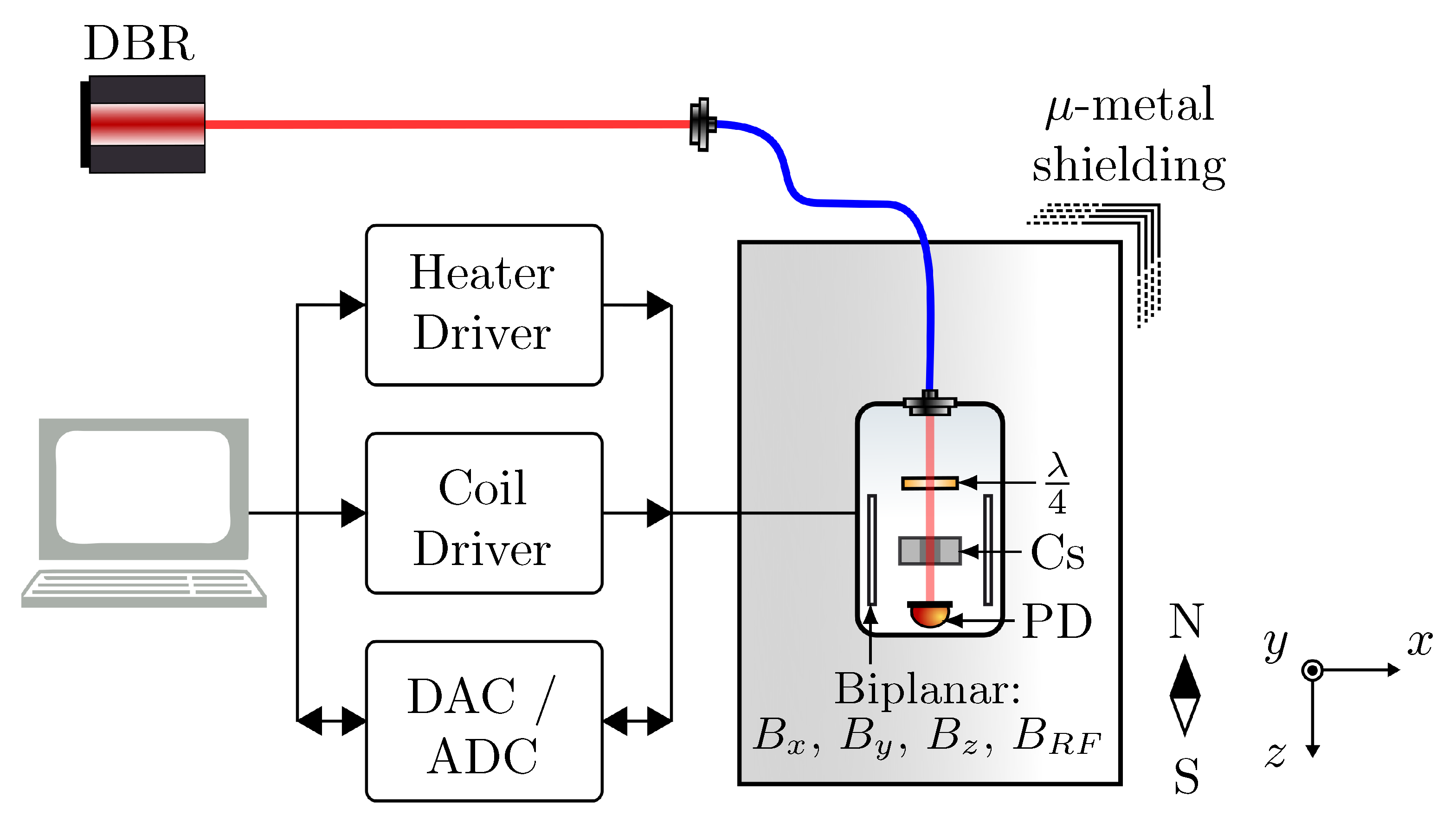
2.1. Experimental Set-Up
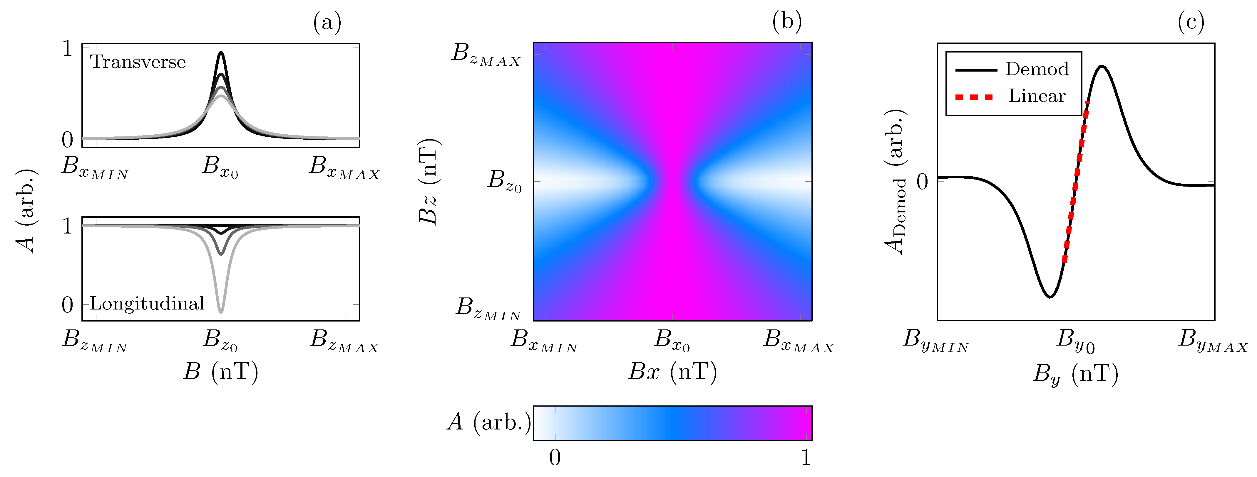
2.2. Hanle Resonance
Machine Learning
2.3. Optimisation Techniques
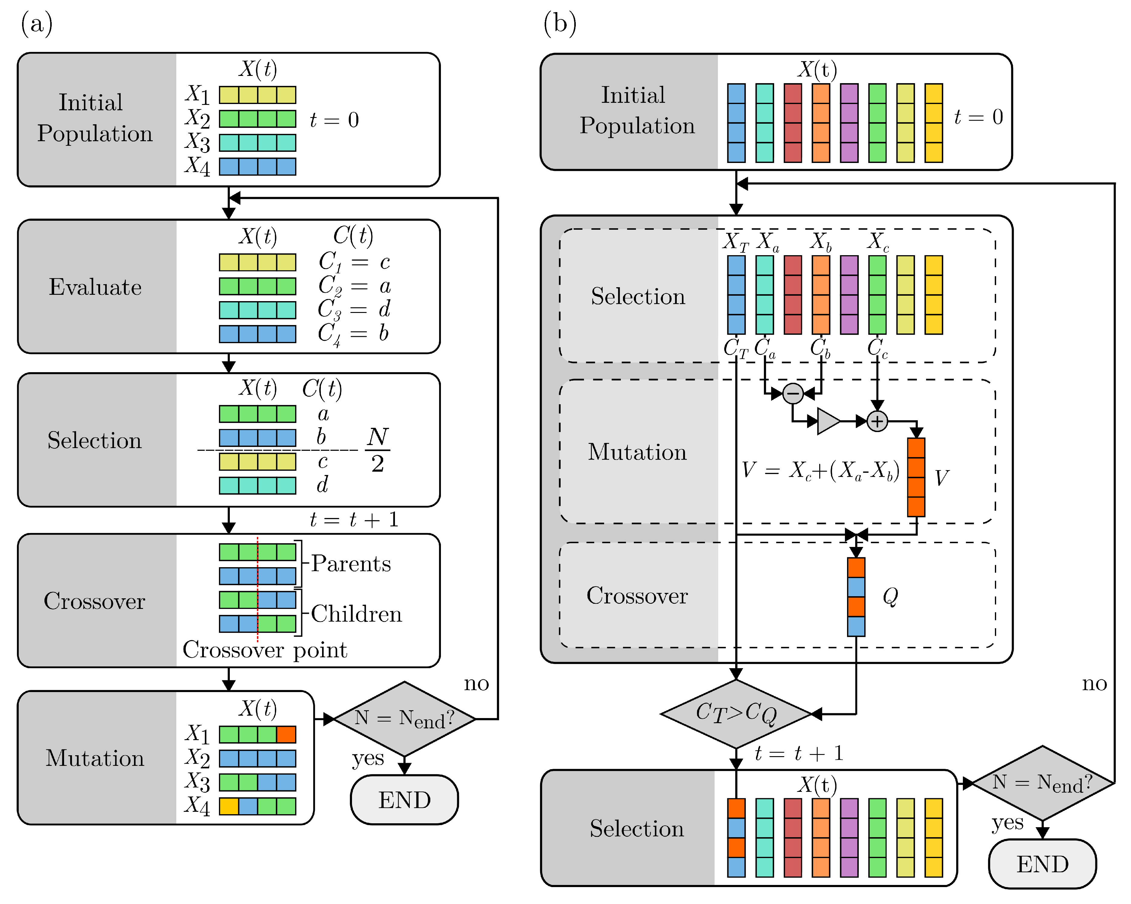
2.3.1. Evolutionary Algorithms
2.3.2. Gradient Ascent
2.3.3. Gaussian Process Regression
2.4. Parameters
3. Results
- Scheme 1.
- Cost = ,
- Scheme 2.
- Cost = ,
- Scheme 3.
- Cost = ,
- Scheme 4.
- Cost = ,
- Scheme 1.
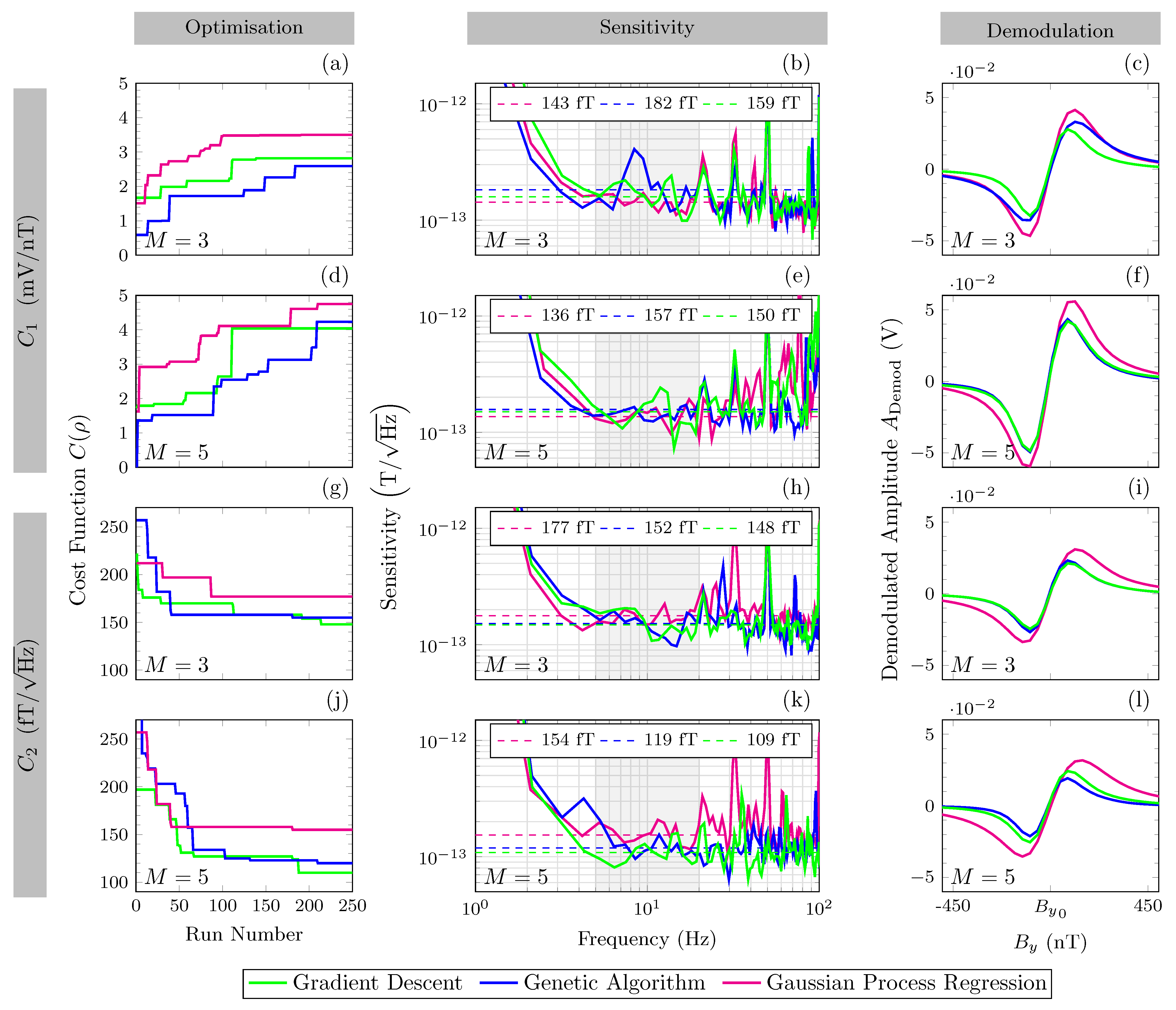
- . All MLAs converged at mV/nT, equating to a measured sensitivity of 163 .
- Scheme 2.
- . All MLAs converged at mV/nT, equating to a measured sensitivity of 147 .
- Scheme 3.
- . All MLAs converged at a measured sensitivity of 163 , equating to a demodulated gradient of mV/nT.
- Scheme 4.
- . All MLAs converged at a measured sensitivity of 132 , equating to a demodulated gradient of mV/nT.
4. Discussion
Author Contributions
Funding
Institutional Review Board Statement
Informed Consent Statement
Data Availability Statement
Acknowledgments
Conflicts of Interest
References
- Boto, E.; Holmes, N.; Leggett, J.; Roberts, G.; Shah, V.; Meyer, S.S.; Muñoz, L.D.; Mullinger, K.J.; Tierney, T.M.; Bestmann, S.; et al. Moving magnetoencephalography towards real-world applications with a wearable system. Nature 2018, 555, 657–661. [Google Scholar] [CrossRef] [PubMed]
- Hill, R.M.; Boto, E.; Holmes, N.; Hartley, C.; Seedat, Z.A.; Leggett, J.; Roberts, G.; Shah, V.; Tierney, T.M.; Woolrich, M.W.; et al. A tool for functional brain imaging with lifespan compliance. Nat. Commun. 2019, 10, 1–11. [Google Scholar] [CrossRef] [PubMed]
- Limes, M.E.; Foley, E.L.; Kornack, T.W.; Caliga, S.; McBride, S.; Braun, A.; Lee, W.; Lucivero, V.G.; Romalis, M.V. Portable magnetometry for detection of biomagnetism in ambient environments. Phys. Rev. Appl. 2020, 14, 011002. [Google Scholar] [CrossRef]
- Zhang, R.; Xiao, W.; Ding, Y.; Feng, Y.; Peng, X.; Shen, L.; Sun, C.; Wu, T.; Wu, Y.; Yang, Y.; et al. Recording brain activities in unshielded Earth’s field with optically pumped atomic magnetometers. Sci. Adv. 2020, 6, 8792–8804. [Google Scholar] [CrossRef]
- Ledbetter, M.P.; Savukov, I.M.; Acosta, V.M.; Budker, D.; Romalis, M.V. Spin-exchange-relaxation-free magnetometry with Cs vapor. Phys. Rev. At. Mol. Opt. Phys. 2008, 77, 1–7. [Google Scholar] [CrossRef]
- Sheng, J.; Wan, S.; Sun, Y.; Dou, R.; Guo, Y.; Wei, K.; He, K.; Qin, J.; Gao, J.H. Magnetoencephalography with a Cs-based high-sensitivity compact atomic magnetometer. Rev. Sci. Instrum. 2017, 88, 094304. [Google Scholar] [CrossRef] [PubMed]
- Chen, Y.; Chen, Y.; Zhao, L.; Zhang, N.; Yu, M.; Ma, Y.; Han, X.; Zhao, M.; Lin, Q.; Yang, P.; et al. Single beam Cs-Ne SERF atomic magnetometer with the laser power differential method. Opt. Express 2022, 30, 16541–16552. [Google Scholar] [CrossRef]
- Fang, J.; Li, R.; Duan, L.; Chen, Y.; Quan, W. Study of the operation temperature in the spin-exchange relaxation free magnetometer. Rev. Sci. Instrum. 2015, 86, 73116. [Google Scholar] [CrossRef]
- Li, Q.; Zhang, J.; Li, L.; Zeng, X.; Sun, W. The effects of phase retardation of wave plate on cesium magnetometer sensitivity. Proc. Appl. Mech. Mater. 2012, 203, 263–267. [Google Scholar] [CrossRef]
- Castagna, N.; Weis, A. Measurement of longitudinal and transverse spin relaxation rates using the ground-state Hanle effect. Phys. Rev. At. Mol. Opt. Phys. 2011, 84, 1–11. [Google Scholar] [CrossRef]
- Recknagel, F. Applications of machine learning to ecological modelling. Ecol. Model. 2001, 146, 303–310. [Google Scholar] [CrossRef]
- Rajkomar, A.; Dean, J.; Kohane, I. Machine Learning in Medicine. N. Engl. J. Med. 2019, 380, 1347–1358. [Google Scholar] [CrossRef] [PubMed]
- Chen, J.; Wu, Z.; Bao, G.; Chen, L.Q.; Zhang, W. Design of coaxial coils using hybrid machine learning. Rev. Sci. Instrum. 2021, 92, 045103. [Google Scholar] [CrossRef] [PubMed]
- Horvitz, E.; Mulligan, D. Data, privacy, and the greater good. Science 2015, 349, 253–255. [Google Scholar] [CrossRef] [PubMed]
- Deans, C.; Griffin, L.D.; Marmugi, L.; Renzoni, F. Machine Learning Based Localization and Classification with Atomic Magnetometers. Phys. Rev. Lett. 2018, 120, 033204. [Google Scholar] [CrossRef]
- Meng, X.; Zhang, Y.; Zhang, X.; Jin, S.; Wang, T.; Jiang, L.; Xiao, L.; Jia, S.; Xiao, Y. Machine Learning Assisted Vector Atomic Magnetometry. arXiv 2022, arXiv:2301.05707. [Google Scholar]
- Carleo, G.; Troyer, M. Solving the quantum many-body problem with artificial neural networks. Science 2017, 355, 602–606. [Google Scholar] [CrossRef]
- Seif, A.; Landsman, K.A.; Linke, N.M.; Figgatt, C.; Monroe, C.; Hafezi, M. Machine learning assisted readout of trapped-ion qubits. J. Phys. At. Mol. Opt. Phys. 2018, 51, 174006. [Google Scholar] [CrossRef]
- Nakamura, I.; Kanemura, A.; Nakaso, T.; Yamamoto, R.; Fukuhara, T. Non-standard trajectories found by machine learning for evaporative cooling of 87 Rb atoms. Opt. Express 2019, 27, 20435. [Google Scholar] [CrossRef]
- Wigley, P.B.; Everitt, P.J.; Van Den Hengel, A.; Bastian, J.W.; Sooriyabandara, M.A.; Mcdonald, G.D.; Hardman, K.S.; Quinlivan, C.D.; Manju, P.; Kuhn, C.C.; et al. Fast machine-learning online optimization of ultra-cold-atom experiments. Sci. Rep. 2016, 6, 25890. [Google Scholar] [CrossRef]
- Tranter, A.D.; Slatyer, H.J.; Hush, M.R.; Leung, A.C.; Everett, J.L.; Paul, K.V.; Vernaz-Gris, P.; Lam, P.K.; Buchler, B.C.; Campbell, G.T. Multiparameter optimisation of a magneto-optical trap using deep learning. Nat. Commun. 2018, 9, 00654. [Google Scholar] [CrossRef] [PubMed]
- Wu, Y.; Meng, Z.; Wen, K.; Mi, C.; Zhang, J.; Zhai, H. Active Learning Approach to Optimization of Experimental Control. Chin. Phys. Lett. 2020, 37, 11804. [Google Scholar] [CrossRef]
- Barker, A.J.; Style, H.; Luksch, K.; Sunami, S.; Garrick, D.; Hill, F.; Foot, C.J.; Bentine, E. Applying machine learning optimization methods to the production of a quantum gas. Mach. Learn. Sci. Technol. 2020, 1, 015007. [Google Scholar] [CrossRef]
- Shah, V.; Knappe, S.; Schwindt, P.D.; Kitching, J. Subpicotesla atomic magnetometry with a microfabricated vapour cell. Nat. Photonics 2007, 1, 649–652. [Google Scholar] [CrossRef]
- Dyer, S.; Griffin, P.F.; Arnold, A.S.; Mirando, F.; Burt, D.P.; Riis, E.; Mcgilligan, J.P. Micro-machined deep silicon atomic vapor cells. J. Appl. Phys. 2022, 132, 134401. [Google Scholar] [CrossRef]
- Dawson, R.; O’Dwyer, C.; Mrozowski, M.S.; Irwin, E.; McGilligan, J.P.; Burt, D.P.; Hunter, D.; Ingleby, S.; Griffin, P.F.; Riis, E. A Portable Single-Beam Caesium Zero-Field Magnetometer for Biomagnetic Sensing. arXiv 2023, arXiv:2303.15974. [Google Scholar]
- Mrozowski, M.S.; Chalmers, I.C.; Ingleby, S.J.; Griffin, P.F.; Riis, E. Ultra-low noise, bi-polar, programmable current sources. Rev. Sci. Instrum. 2023, 94, 1–9. [Google Scholar] [CrossRef]
- Zetter, R.; Mäkinen, A.J.; Iivanainen, J.; Zevenhoven, K.C.J.; Ilmoniemi, R.J.; Parkkonen, L. Magnetic field modeling with surface currents. Part II. Implementation and usage of bfieldtools. J. Appl. Phys. 2020, 128, 063905. [Google Scholar] [CrossRef]
- lMakinen, A.J.; Zetter, R.; Iivanainen, J.; Zevenhoven, K.C.J.; Parkkonen, L.; Ilmoniemi, R.J. Magnetic-field modeling with surface currents. Part I. Physical and computational principles of bfieldtools. J. Appl. Phys. 2020, 128, 063906. [Google Scholar] [CrossRef]
- Breschi, E.; Weis, A. Ground-state Hanle effect based on atomic alignment. Phys. Rev. A 2012, 86, 053427. [Google Scholar] [CrossRef]
- Siddique, N.; Adeli, H. Nature Inspired Computing: An Overview and Some Future Directions. Cogn. Comput. 2015, 7, 706–714. [Google Scholar] [CrossRef]
- Slowik, A.; Kwasnicka, H. Evolutionary algorithms and their applications to engineering problems. Neural Comput. Appl. 2020, 32, 12363–12379. [Google Scholar] [CrossRef]
- Ruder, S. An overview of gradient descent optimization algorithms. arXiv 2016, arXiv:1609.04747. [Google Scholar]
- Darken, C.; Chang, J.; Moody, J. Original appears in Neural Networks for Signal Processing 2. In Proceedings of the 1992 IEEE Workshop, Seattle, WA, USA, 15–18 September 1992. [Google Scholar]
- Sweke, R.; Wilde, F.; Meyer, J.J.; Schuld, M.; Fährmann, P.K.; Meynard-Piganeau, B.; Eisert, J. Stochastic gradient descent for hybrid quantum-classical optimization. Quantum 2020, 4, 01155. [Google Scholar] [CrossRef]
- Khaneja, N.; Reiss, T.; Kehlet, C.; Schulte-Herbrüggen, T.; Glaser, S.J. Optimal control of coupled spin dynamics: Design of NMR pulse sequences by gradient ascent algorithms. J. Magn. Reson. 2005, 172, 296–305. [Google Scholar] [CrossRef] [PubMed]
- Seltzer, S.J. Developments in alkali-metal atomic magnetometry. Ph.D. Thesis, Princeton University, Princeton, NJ, USA, 2008. [Google Scholar]
- Yin, Y.; Zhou, B.; Wang, Y.; Ye, M.; Ning, X.; Han, B.; Fang, J. The influence of modulated magnetic field on light absorption in SERF atomic magnetometer. Rev. Sci. Instrum. 2022, 93, 13001. [Google Scholar] [CrossRef]


| Parameter | Min (p) | Max (p) | Default (p) | Unit |
|---|---|---|---|---|
| Temperature | 115 | 140 | - | C |
| Laser Power | 0.5 | 6 | - | mW |
| Laser Detuning | −20 | 20 | - | GHz |
| 0.2 | 1.5 | 0.5 | dimensionless | |
| 0.2 | 1.5 | 1 | dimensionless |
| MLA | M | T | LD | LP | |||||||
|---|---|---|---|---|---|---|---|---|---|---|---|
| GD | 3 | 2.82 ± 0.03 | 158.62 ± 1.3 | 132.51 ± 1.5 | 119.41 | 8.24 | 6.00 | 0.50 | 1.00 | 0.55 | |
| GA | 3 | 2.59 ± 0.02 | 182.39 ± 1.4 | 183.27 ± 2.1 | 115.00 | 3.00 | 5.35 | 0.50 | 1.00 | 0.55 | |
| GP | 3 | 3.50 ± 0.03 | 143.40 ± 1.2 | 168.83 ± 1.6 | 115.00 | 8.00 | 6.00 | 0.50 | 1.00 | 0.55 | |
| GD | 5 | 4.04 ± 0.02 | 150.24 ± 1.5 | 130.06 ± 2.1 | 118.85 | 10.77 | 5.58 | 1.50 | 0.30 | 5.51 | |
| GA | 5 | 4.23 ± 0.02 | 157.62 ± 1.3 | 98.81 ± 2.0 | 123.00 | 7.00 | 5.32 | 1.48 | 0.39 | 4.21 | |
| GP | 5 | 4.75 ± 0.03 | 136.30 ± 1.2 | 147.36 ± 1.2 | 120.13 | 6.22 | 6.00 | 1.50 | 0.21 | 7.82 | |
| GD | 3 | 2.10 ± 0.02 | 148.28 ± 1.3 | 143.36 ± 2.5 | 117.94 | 5.88 | 5.35 | 0.50 | 1.00 | 0.55 | |
| GA | 3 | 2.35 ± 0.02 | 152.30 ± 1.3 | 136.66 ± 1.3 | 119.00 | 4.00 | 4.66 | 0.50 | 1.00 | 0.55 | |
| GP | 3 | 2.31 ± 0.02 | 177.40 ± 1.3 | 192.81 ± 1.6 | 115.01 | 3.49 | 5.57 | 0.50 | 1.00 | 0.55 | |
| GD | 5 | 2.22 ± 0.03 | 109.59 ± 1.3 | 137.70 ± 1.6 | 118.85 | 7.69 | 5.58 | 0.70 | 0.80 | 0.96 | |
| GA | 5 | 1.95 ± 0.02 | 119.76 ± 1.2 | 111.05 ± 2.1 | 121.00 | 7.00 | 5.24 | 0.97 | 1.15 | 0.93 | |
| GP | 5 | 3.65 ± 0.02 | 154.81 ± 1.2 | 203.05 ± 1.6 | 115.00 | 3.00 | 5.50 | 1.09 | 1.00 | 1.20 |
Disclaimer/Publisher’s Note: The statements, opinions and data contained in all publications are solely those of the individual author(s) and contributor(s) and not of MDPI and/or the editor(s). MDPI and/or the editor(s) disclaim responsibility for any injury to people or property resulting from any ideas, methods, instructions or products referred to in the content. |
© 2023 by the authors. Licensee MDPI, Basel, Switzerland. This article is an open access article distributed under the terms and conditions of the Creative Commons Attribution (CC BY) license (https://creativecommons.org/licenses/by/4.0/).
Share and Cite
Dawson, R.; O’Dwyer, C.; Irwin, E.; Mrozowski, M.S.; Hunter, D.; Ingleby, S.; Riis, E.; Griffin, P.F. Automated Machine Learning Strategies for Multi-Parameter Optimisation of a Caesium-Based Portable Zero-Field Magnetometer. Sensors 2023, 23, 4007. https://doi.org/10.3390/s23084007
Dawson R, O’Dwyer C, Irwin E, Mrozowski MS, Hunter D, Ingleby S, Riis E, Griffin PF. Automated Machine Learning Strategies for Multi-Parameter Optimisation of a Caesium-Based Portable Zero-Field Magnetometer. Sensors. 2023; 23(8):4007. https://doi.org/10.3390/s23084007
Chicago/Turabian StyleDawson, Rach, Carolyn O’Dwyer, Edward Irwin, Marcin S. Mrozowski, Dominic Hunter, Stuart Ingleby, Erling Riis, and Paul F. Griffin. 2023. "Automated Machine Learning Strategies for Multi-Parameter Optimisation of a Caesium-Based Portable Zero-Field Magnetometer" Sensors 23, no. 8: 4007. https://doi.org/10.3390/s23084007
APA StyleDawson, R., O’Dwyer, C., Irwin, E., Mrozowski, M. S., Hunter, D., Ingleby, S., Riis, E., & Griffin, P. F. (2023). Automated Machine Learning Strategies for Multi-Parameter Optimisation of a Caesium-Based Portable Zero-Field Magnetometer. Sensors, 23(8), 4007. https://doi.org/10.3390/s23084007