Author Contributions
Conceptualization, V.H. and B.S.; methodology, V.H.; software, V.H.; formal analysis, V.H.; investigation, V.H.; data curation, V.H.; writing—original draft preparation, V.H.; writing—review and editing, V.H., P.P.-P., B.S. and O.S.; visualization, V.H.; supervision, P.P.-P., B.S. and O.S. All authors have read and agreed to the published version of the manuscript.
Figure 1.
Low-cost GNSS receiver simpleRTK2B V1 (in front), Survey calibrated low-cost antenna (left), and Javad RingAnt-G3T geodetic antenna (right).
Figure 1.
Low-cost GNSS receiver simpleRTK2B V1 (in front), Survey calibrated low-cost antenna (left), and Javad RingAnt-G3T geodetic antenna (right).
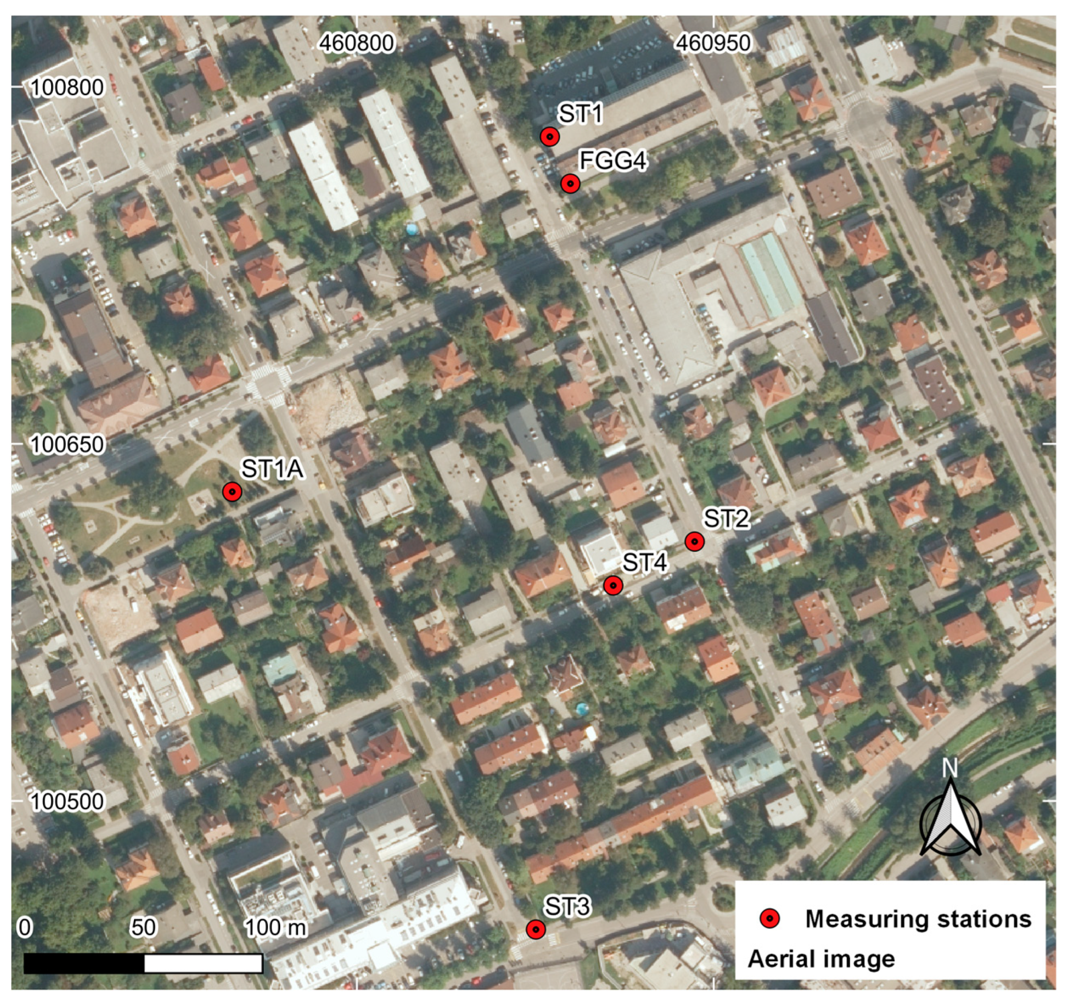
Figure 2.
Measuring stations.
Figure 2.
Measuring stations.
Figure 3.
Location of measuring stations: (a) LC−1, LC−2, and GD−1 in ST 1; (b) LC−1, LC−2, and GD−1 in ST 1A; (c) LC−1 in ST 2; (d) LC−1 in ST 3; and (e) LC−1 in ST 4.
Figure 3.
Location of measuring stations: (a) LC−1, LC−2, and GD−1 in ST 1; (b) LC−1, LC−2, and GD−1 in ST 1A; (c) LC−1 in ST 2; (d) LC−1 in ST 3; and (e) LC−1 in ST 4.
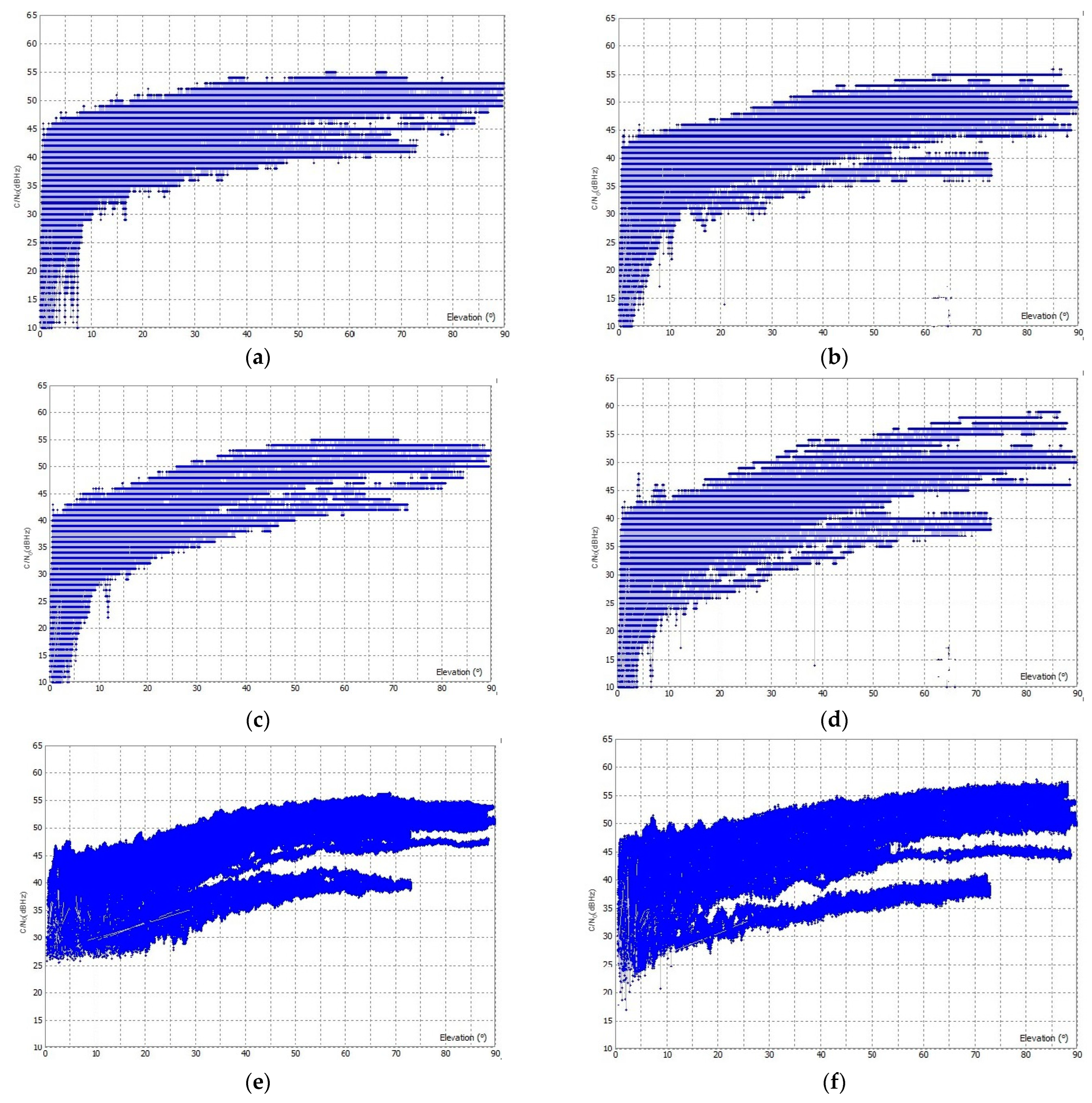
Figure 4.
C/N0 for observations in F1 and F2 frequency in the open sky: (a) F1 C/N0 for LC−1, (b) F2 C/N0 for LC−1, (c) F1 C/N0 for LC−2, (d) F2 C/N0 for LC−2, (e) F1 C/N0 for GD−1, and (f) F2 C/N0 for GD−1.
Figure 4.
C/N0 for observations in F1 and F2 frequency in the open sky: (a) F1 C/N0 for LC−1, (b) F2 C/N0 for LC−1, (c) F1 C/N0 for LC−2, (d) F2 C/N0 for LC−2, (e) F1 C/N0 for GD−1, and (f) F2 C/N0 for GD−1.
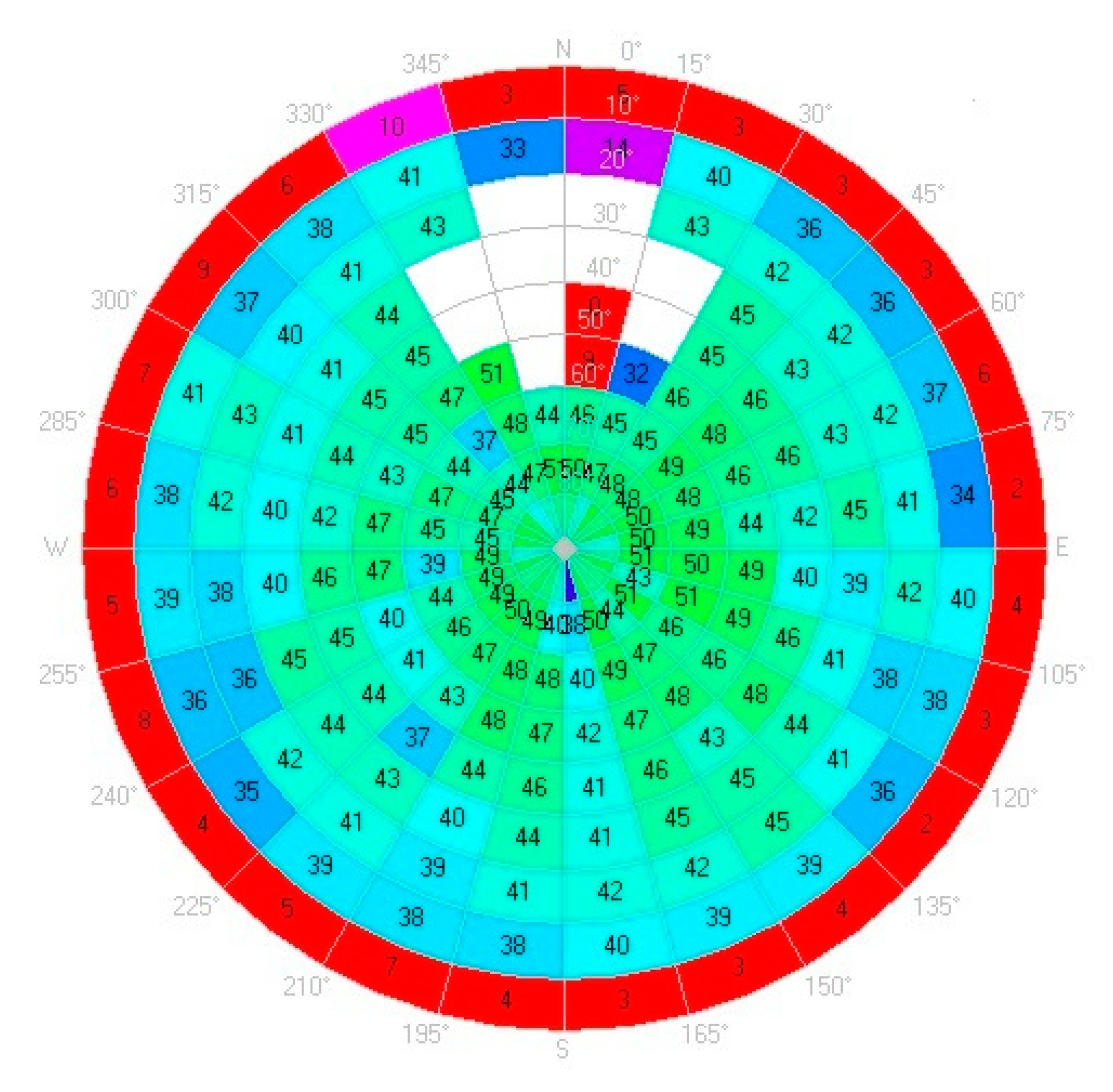
Figure 5.
Sky plot of C/N0 for LC−1.
Figure 5.
Sky plot of C/N0 for LC−1.
Figure 6.
C/N0 for observations in F1 and F2 frequency in the urban areas: (a) F1 C/N0 for LC−1, (b) F2 C/N0 for LC−1, (c) F1 C/N0 for LC−2, (d) F2 C/N0 for LC−2, (e) F1 C/N0 for GD−1, and (f) F2 C/N0 for GD−1.
Figure 6.
C/N0 for observations in F1 and F2 frequency in the urban areas: (a) F1 C/N0 for LC−1, (b) F2 C/N0 for LC−1, (c) F1 C/N0 for LC−2, (d) F2 C/N0 for LC−2, (e) F1 C/N0 for GD−1, and (f) F2 C/N0 for GD−1.
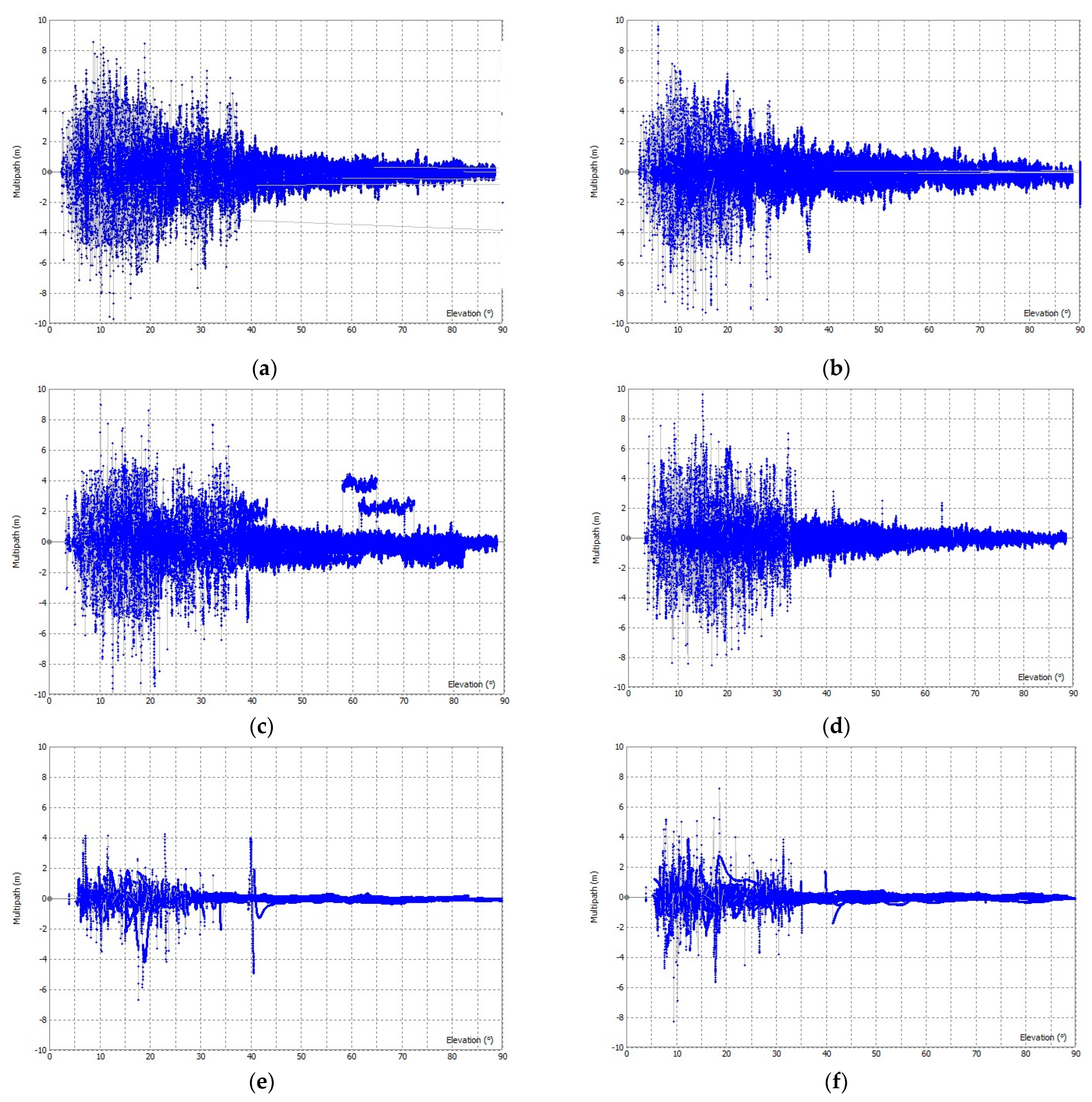
Figure 7.
Multipath for code observations in F1 and F2 frequency in the open sky: (a) F1 multipath for LC−1, (b) F2 multipath for LC−1, (c) F1 multipath for LC−2, (d) F2 multipath for LC−2, (e) F1 multipath for GD−1, and (f) F2 multipath for GD−1.
Figure 7.
Multipath for code observations in F1 and F2 frequency in the open sky: (a) F1 multipath for LC−1, (b) F2 multipath for LC−1, (c) F1 multipath for LC−2, (d) F2 multipath for LC−2, (e) F1 multipath for GD−1, and (f) F2 multipath for GD−1.
Figure 8.
Multipath for code observations in F1 and F2 frequency in urban areas: (a) F1 multipath for LC−1, (b) F2 multipath for LC−1, (c) F1 multipath for LC−2, (d) F2 multipath for LC−2, (e) F1 multipath for GD−1, and (f) F2 multipath for GD−1.
Figure 8.
Multipath for code observations in F1 and F2 frequency in urban areas: (a) F1 multipath for LC−1, (b) F2 multipath for LC−1, (c) F1 multipath for LC−2, (d) F2 multipath for LC−2, (e) F1 multipath for GD−1, and (f) F2 multipath for GD−1.
Figure 9.
Positioning solutions in open sky and urban conditions: (a) LC−1 on ST 1 (open sky); (b) LC−2 on ST 1 (open sky); (c) LC−1 on ST 1A (urban areas); and (d) LC−2 on ST 1A (urban areas).
Figure 9.
Positioning solutions in open sky and urban conditions: (a) LC−1 on ST 1 (open sky); (b) LC−2 on ST 1 (open sky); (c) LC−1 on ST 1A (urban areas); and (d) LC−2 on ST 1A (urban areas).
Figure 10.
Horizontal, vertical, and spatial positioning accuracy in the open-sky (ST 1) and urban areas (ST 2, ST 3, ST 4): (a) LC−1 at ST 1; (b) LC−1 at ST 2; (c) LC−1 at ST 3; and (d) LC−1 at ST 4.
Figure 10.
Horizontal, vertical, and spatial positioning accuracy in the open-sky (ST 1) and urban areas (ST 2, ST 3, ST 4): (a) LC−1 at ST 1; (b) LC−1 at ST 2; (c) LC−1 at ST 3; and (d) LC−1 at ST 4.
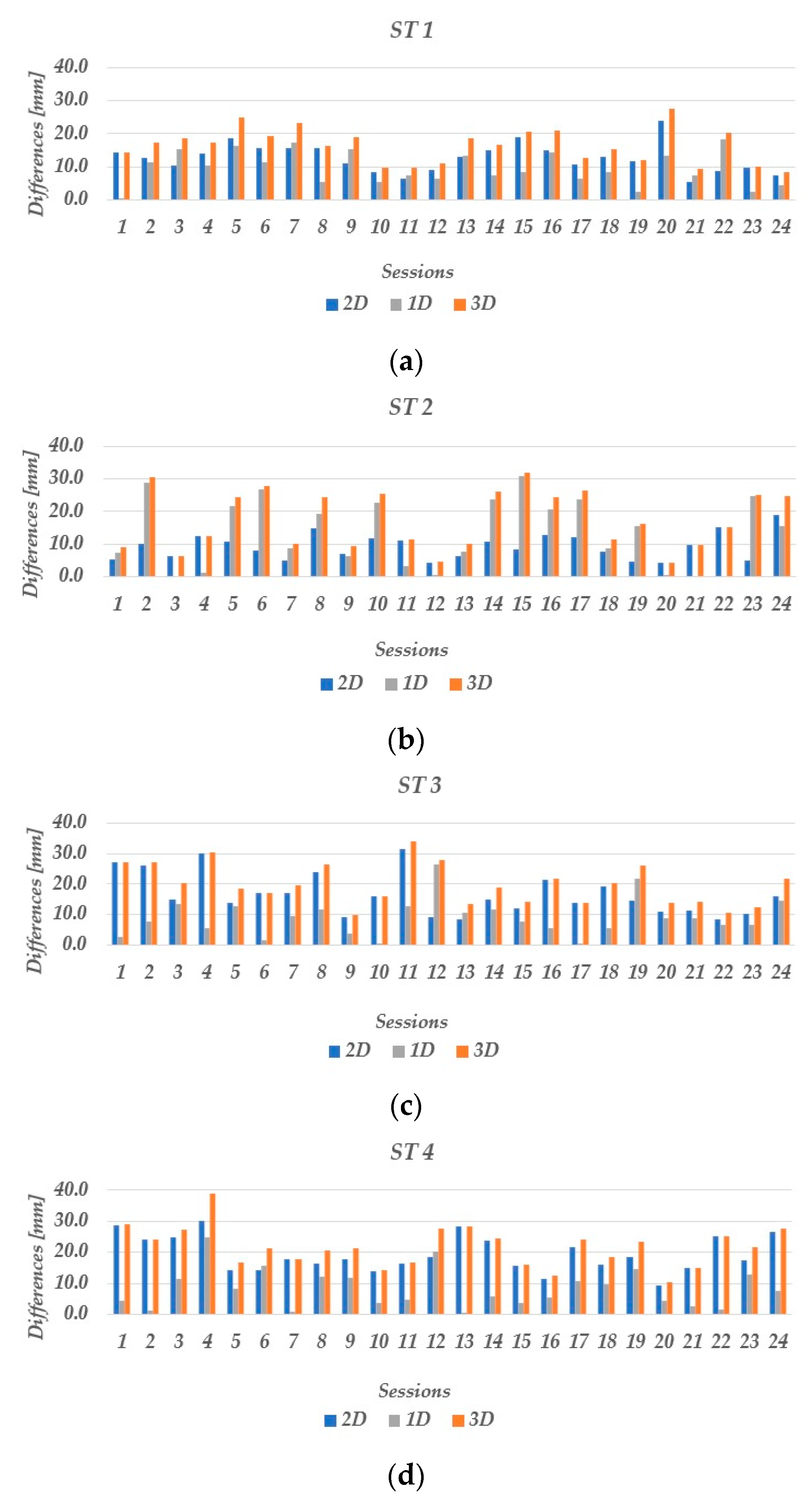
Figure 11.
Horizontal, vertical, and spatial positioning accuracy in the open-sky (ST 1) and urban areas (ST 2, ST 3, ST 4) for 24 sessions: (a) LC−1 at ST 1; (b) LC−1 at ST 2; (c) LC−1 at ST 3; and (d) LC−1 at ST 4.
Figure 11.
Horizontal, vertical, and spatial positioning accuracy in the open-sky (ST 1) and urban areas (ST 2, ST 3, ST 4) for 24 sessions: (a) LC−1 at ST 1; (b) LC−1 at ST 2; (c) LC−1 at ST 3; and (d) LC−1 at ST 4.
Table 1.
Used parameters in the data processing.
Table 1.
Used parameters in the data processing.
| Parameters | RTKLIB |
|---|
| Observations | Phase |
| Duration | 1 h, 30 min, 20 min, and 15 min |
| Constellations | GPS, GLONASS, Galileo |
| Ambiguity | Continuous |
| Elevation mask | 15° |
Table 2.
RMSE for multipath error in open-sky and urban conditions.
Table 2.
RMSE for multipath error in open-sky and urban conditions.
| Scenarios | Frequency | LC−1 | LC−2 | GD−1 |
|---|
| Open sky | F1 | 0.50 m | 0.51 m | 0.16 m |
| | F2 | 0.48 m | 0.57 m | 0.23 m |
| Urban area | F1 | 0.86 m | 0.90 m | 0.23 m |
| | F2 | 0.76 m | 0.70 m | 0.31 m |
Table 3.
Ambiguity resolution ratio for LC−1 and LC−2.
Table 3.
Ambiguity resolution ratio for LC−1 and LC−2.
| Scenarios | Solution | LC−1 | LC−2 |
|---|
| Open sky | Fixed | 96.8% | 98.3% |
| | Float | 3.2 % | 1.7% |
| Urban area | Fixed | 75.0% | 93.4% |
| | Float | 25.0% | 6.6% |
Table 4.
Positioning performance results at ST 1.
Table 4.
Positioning performance results at ST 1.
| Sessions (min) | ƛe (mm) | ƛn (mm) | ƛh (mm) | d2D (mm) | d3D (mm) |
|---|
| 0–60 | 0.7 | −2.8 | −1.3 | 2.9 | 3.2 |
| 0−30 | 0.7 | −2.1 | −1.2 | 2.2 | 2.5 |
| 30–60 | 0.7 | −2.9 | −0.9 | 3.0 | 3.1 |
| 0−20 | 0.1 | −1.1 | −0.4 | 1.1 | 1.2 |
| 20–40 | 1.0 | −3.0 | −1.9 | 3.2 | 3.7 |
| 40−60 | 0.6 | −2.7 | −0.6 | 2.8 | 2.8 |
| 0–15 | 0.2 | −0.5 | −0.9 | 0.5 | 1.0 |
| 15−30 | 0.6 | −2.2 | −0.7 | 2.3 | 2.4 |
| 30–45 | 1.8 | −2.9 | −2.9 | 3.4 | 4.5 |
| 45−60 | 0.6 | −2.6 | −0.7 | 2.7 | 2.8 |
Table 5.
Positioning performance results at ST 2.
Table 5.
Positioning performance results at ST 2.
| | ƛe (mm) | ƛn (mm) | ƛh (mm) | d2D (mm) | d3D (mm) |
|---|
| 0–60 | −0.5 | 0.0 | 8.5 | 0.5 | 8.5 |
| 0–30 | −4.3 | −0.9 | 3.0 | 4.4 | 5.3 |
| 30–60 | 3.2 | −2.1 | 19.8 | 3.8 | 20.2 |
| 0–20 | −5.0 | 2.1 | 11.2 | 5.4 | 12.4 |
| 20–40 | −2.4 | −6.0 | 20.3 | 6.5 | 21.3 |
| 40–60 | 5.4 | −4.5 | 26.3 | 7.0 | 27.2 |
| 0–15 | −5.5 | −15.3 | 14.5 | 16.3 | 21.8 |
| 15–30 | −4.3 | −0.9 | 3.0 | 4.4 | 5.3 |
| 30–45 | −3.3 | 0.7 | 12.5 | 3.4 | 12.9 |
| 45–60 | 10.1 | −0.8 | 20.6 | 10.1 | 23.0 |
Table 6.
Positioning performance results at ST 3.
Table 6.
Positioning performance results at ST 3.
| Sessions (min) | ƛe (mm) | ƛn (mm) | ƛh (mm) | d2D (mm) | d3D (mm) |
|---|
| 0–60 | −4.8 | 0.4 | 10.3 | 4.8 | 11.4 |
| 0−30 | −6.6 | −0.9 | 13.3 | 6.7 | 14.9 |
| 30–60 | −4.8 | 3.5 | 5.2 | 5.9 | 7.9 |
| 0–20 | −6.0 | 0.6 | 6.8 | 6.0 | 9.1 |
| 20–40 | −3.8 | 5.2 | −11.6 | 6.4 | 13.3 |
| 40–60 | −6.4 | −1.3 | 13.6 | 6.5 | 15.1 |
| 0–15 | −6.9 | −4.9 | −9.8 | 8.5 | 12.9 |
| 15–30 | −5.3 | 3.9 | 4.6 | 6.6 | 8.0 |
| 30–45 | −6.3 | 0.7 | 6.4 | 6.3 | 9.0 |
| 45–60 | −4.6 | 1.2 | 13.6 | 4.8 | 14.4 |
Table 7.
Positioning performance results at ST 4.
Table 7.
Positioning performance results at ST 4.
| Sessions (min) | ƛe (mm) | ƛn (mm) | ƛh (mm) | d2D (mm) | d3D (mm) |
|---|
| 0–60 | −8.8 | 8.4 | −1.5 | 12.2 | 12.3 |
| 0–30 | −5.2 | 2.4 | 4.3 | 5.7 | 7.2 |
| 30–60 | −3.3 | 4.4 | 6.9 | 5.5 | 8.8 |
| 0–20 | −8.3 | 0.3 | −6.5 | 8.3 | 10.5 |
| 20–40 | −7.4 | 5.0 | −8.1 | 8.9 | 12.1 |
| 40–60 | / | / | / | / | / |
| 0–15 | −6.1 | 2.7 | 10.4 | 6.7 | 12.4 |
| 15–30 | −10.7 | 5.7 | −18.6 | 12.1 | 22.2 |
| 30–45 | −3.3 | 4.4 | 6.9 | 5.5 | 8.8 |
| 45–60 | / | / | / | / | / |
Table 8.
RTK positioning precision in the open-sky (ST 1) and urban areas (ST 2, ST 3, and ST 4).
Table 8.
RTK positioning precision in the open-sky (ST 1) and urban areas (ST 2, ST 3, and ST 4).
| Station | e (mm) | n (mm) | h (mm) | d2D (mm) | d3D (mm) |
|---|
| ST1 | 3.4 | 5.3 | 5.1 | 6.4 | 8.1 |
| ST2 | 6.5 | 6.5 | 13.5 | 9.2 | 16.3 |
| ST3 | 7.2 | 6.7 | 7.3 | 9.8 | 12.2 |
| ST4 | 6.0 | 8.4 | 10.0 | 10.3 | 14.4 |


