


WiTransformer: A Novel Robust Gesture Recognition Sensing Model with WiFi


Abstract
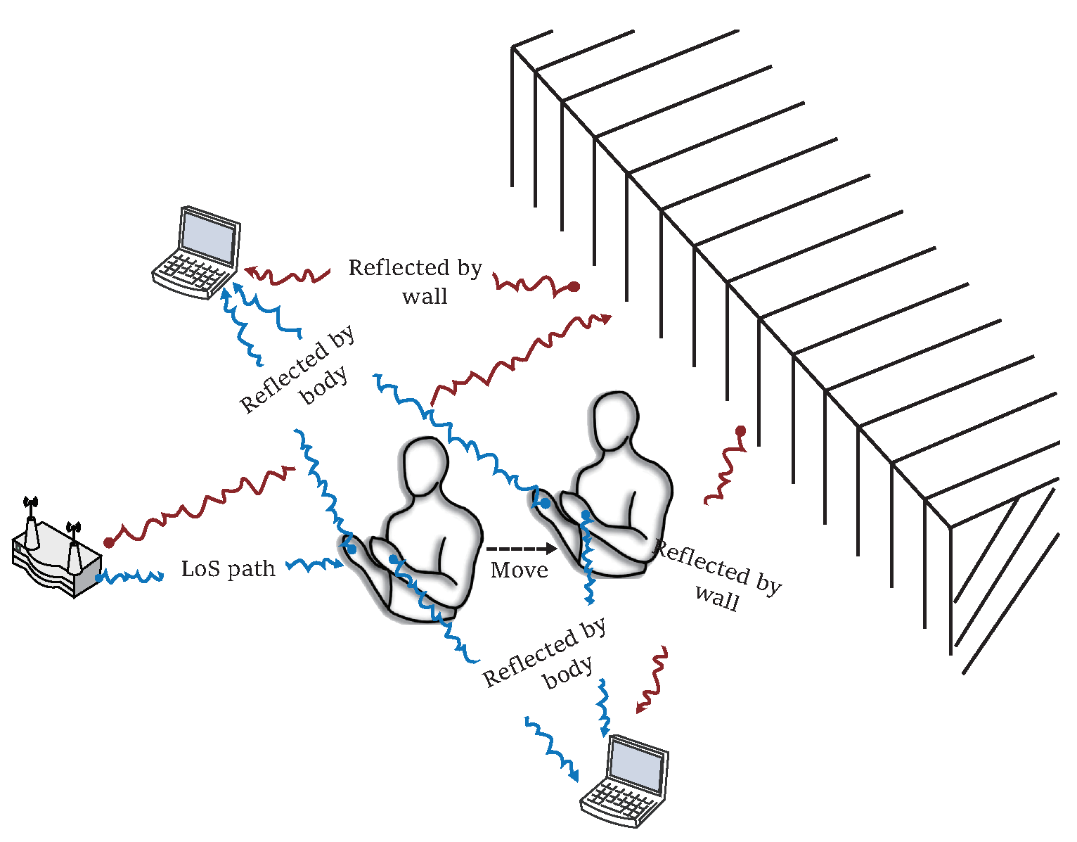
1. Introduction
- To improve the identification of spatiotemporal features and enhance the robustness for recognition task complexity changes, we explore and design two types of three-dimensional (3D) spatiotemporal feature extractors, the united spatiotemporal transformer model (UST) and the separated spatiotemporal transformer model (SST), based on pure modified transformer encoders;
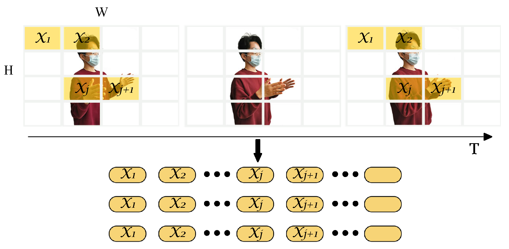
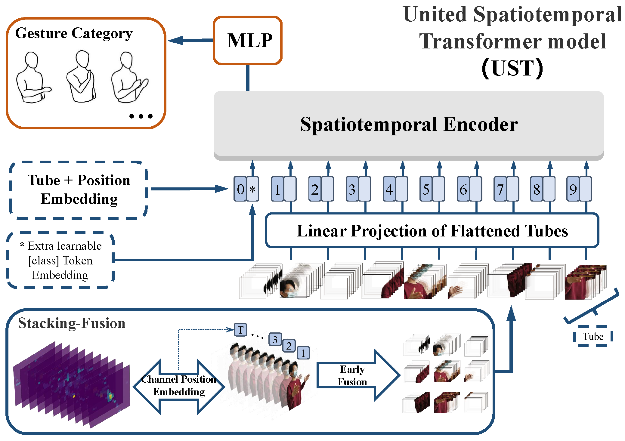
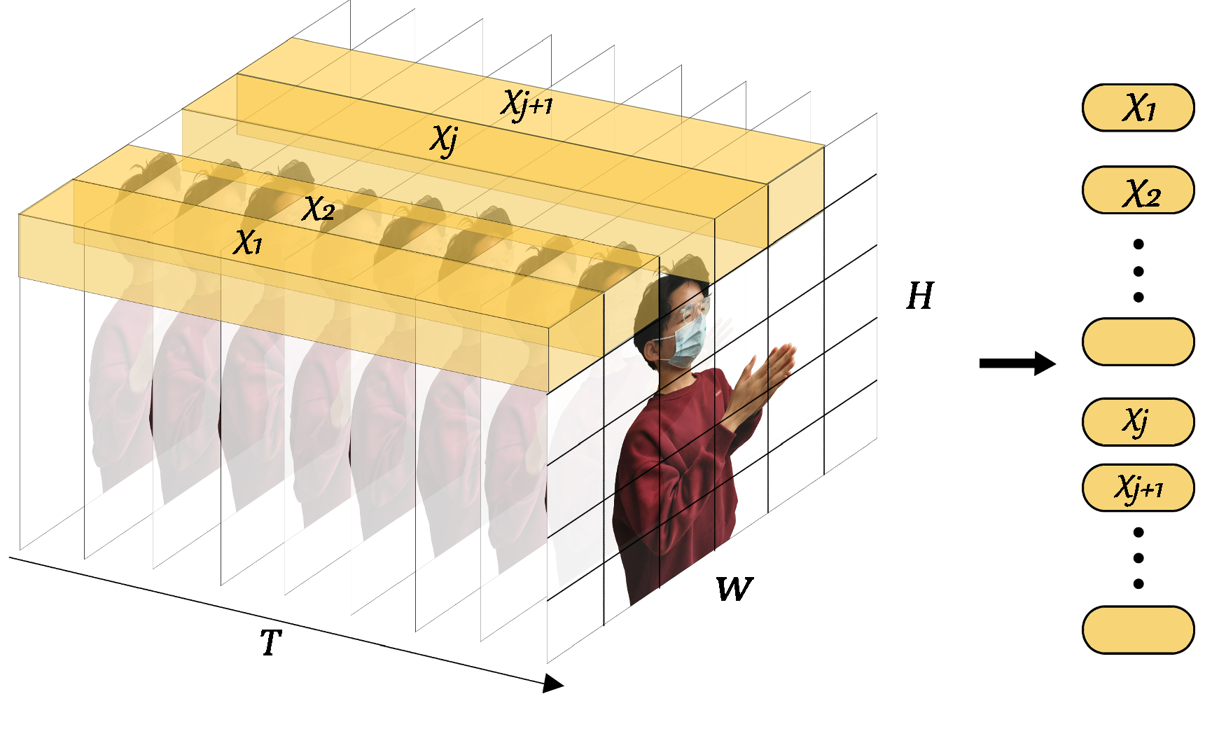
- For UST, we propose a 3D spatiotemporal feature fusion method, stacking-fusion, and tube embedding, which fully simplifies the Transformer-like spatiotemporal fusion architecture and reduces the time complexity. Moreover, the 3D spatiotemporal feature fusion and modeling are realized only by a one-dimensional (1D) encoder;
- We also propose a novel 3D time-series marking strategy, channel position embedding (CPE), for UST to supplement the absence of position information between different BVP input frames;
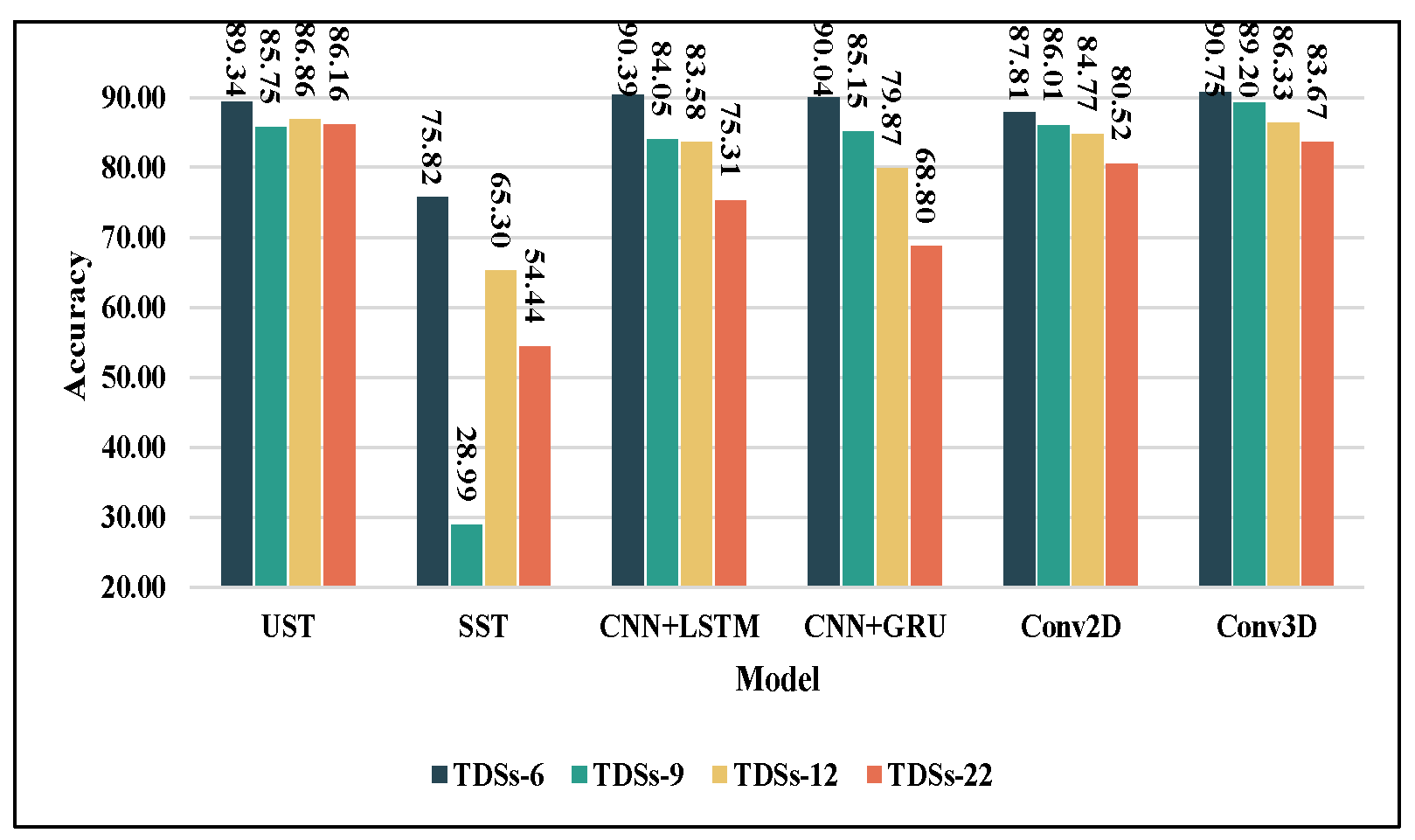
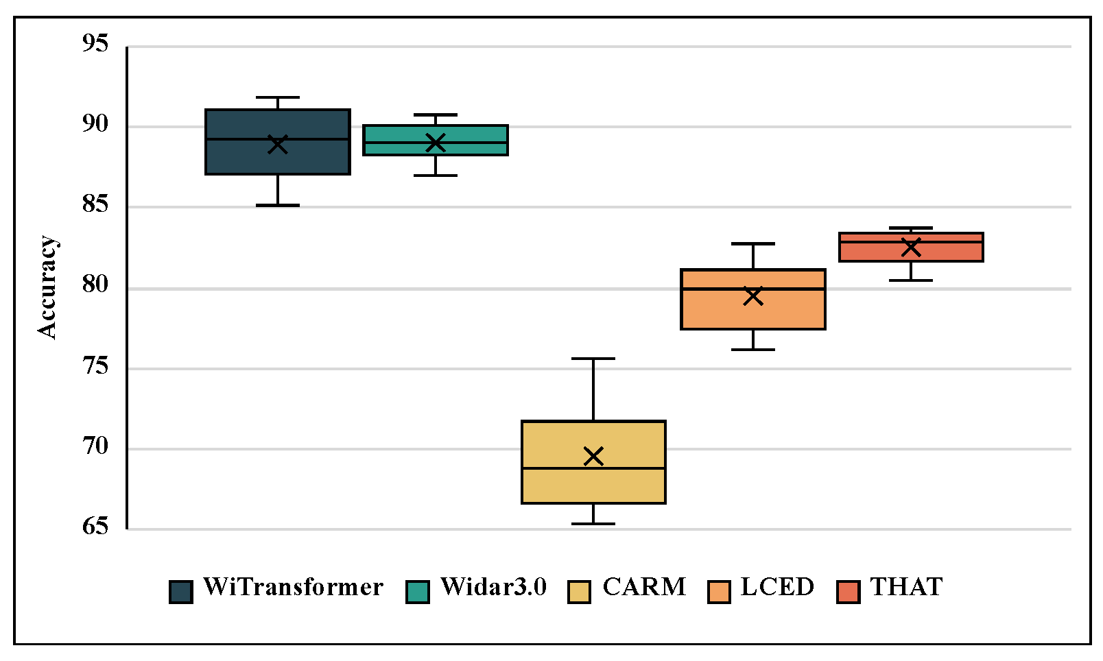
- We conducted experiments on regrouped Widar 3.0 public datasets. The results demonstrated that the UST of WiTransformer, as a category of the backbone network, has higher recognition accuracy and better robustness against the task complexity change compared with other popular models with the ability of 3D-feature extraction (e.g., Conv3D and CNN+GRU). In addition, for the task containing simultaneously three types of task complexity, UST also achieves 89.34% average recognition accuracy outperforming state-of-the-art works (including Widar 3.0, THAT, LCED, and CARM).
2. Related Works
2.1. Expert Knowledge-Driven Method
2.2. Data-Driven Method
2.3. Transformer and Attention
3. Preliminary
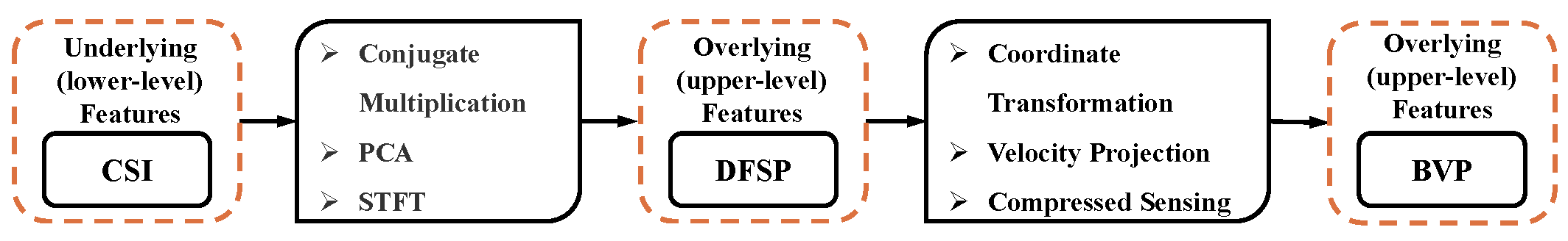
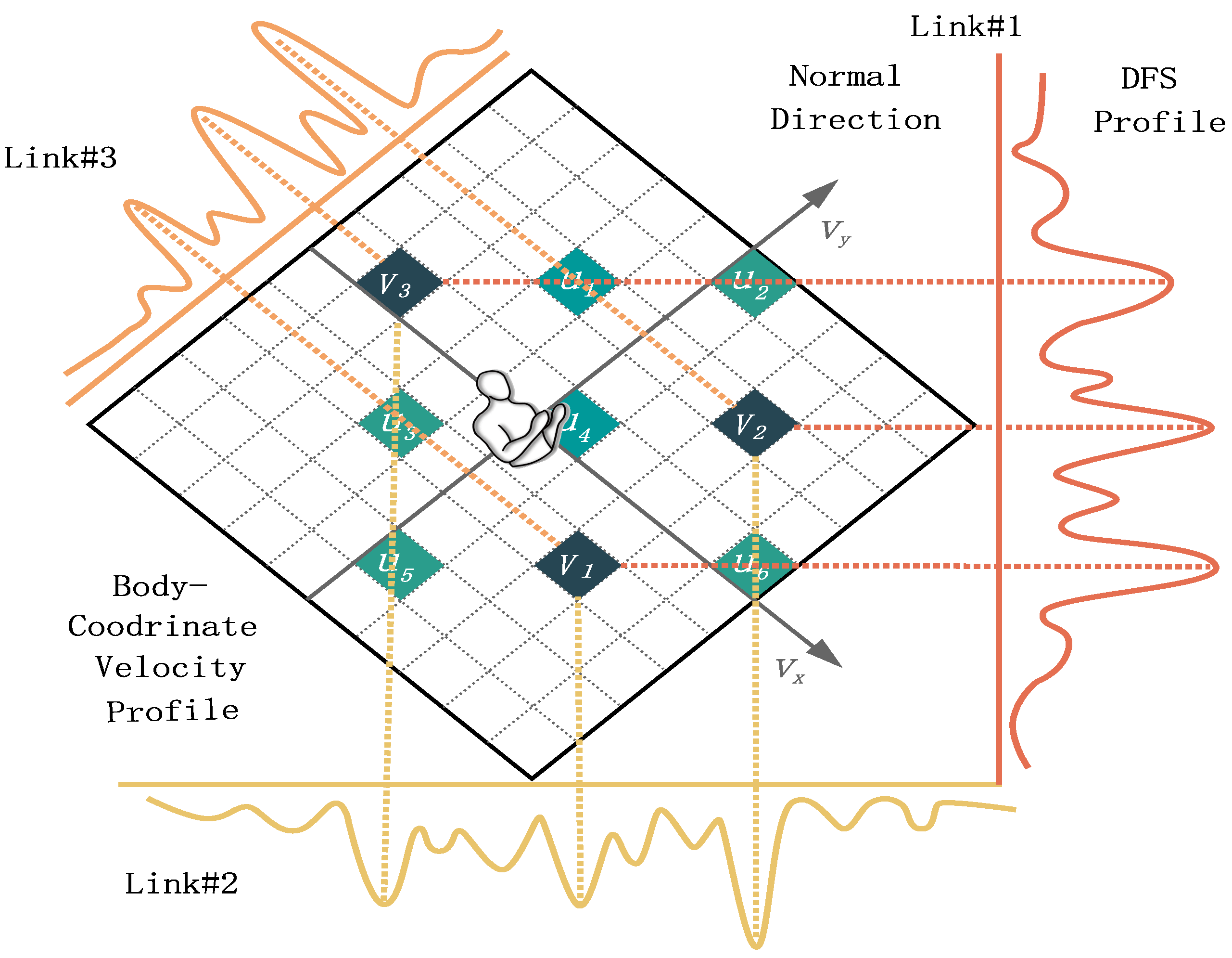
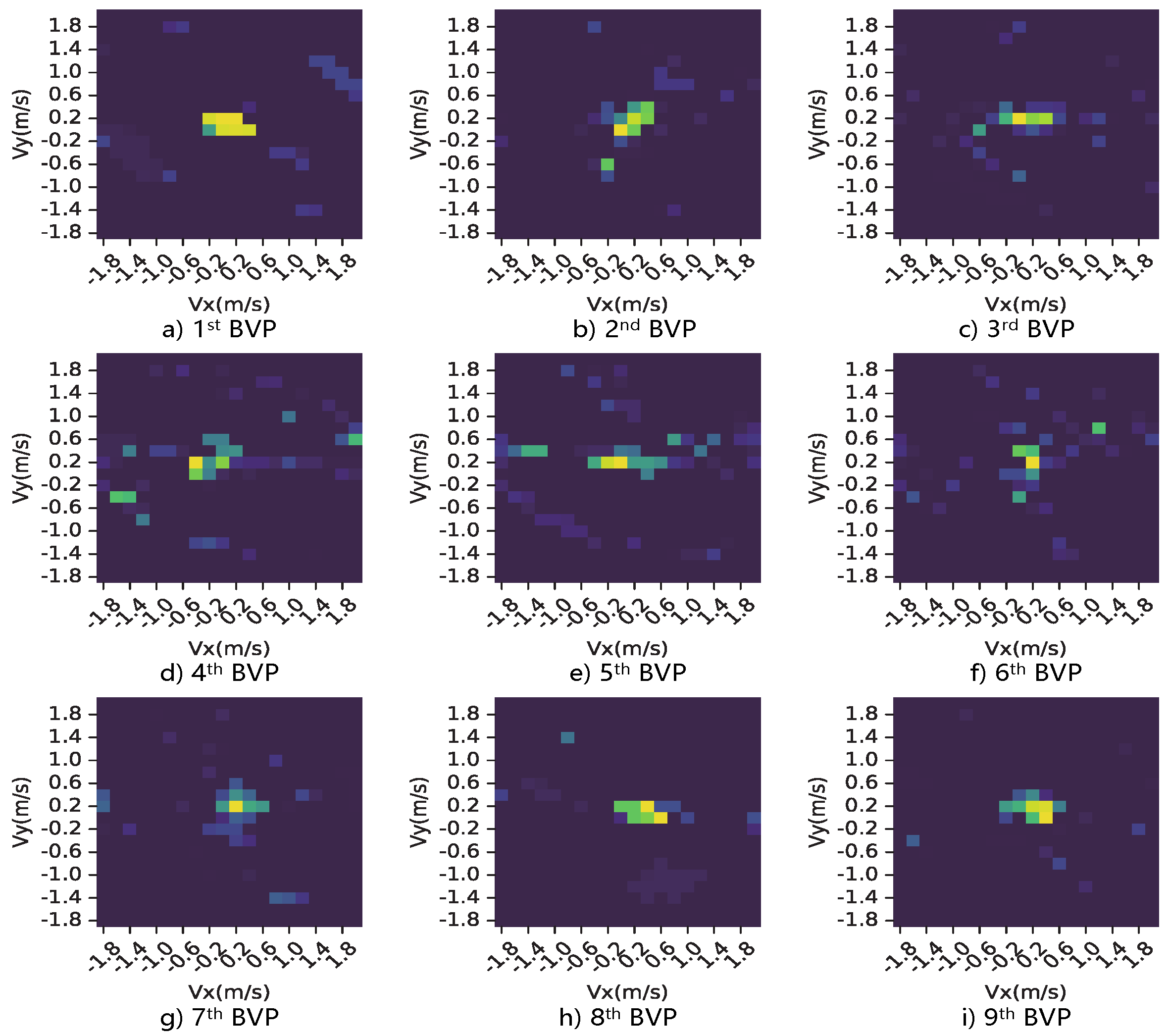
3.1. From CSI to BVP
3.2. Multi-Head Self-Attention
4. WiTransformer
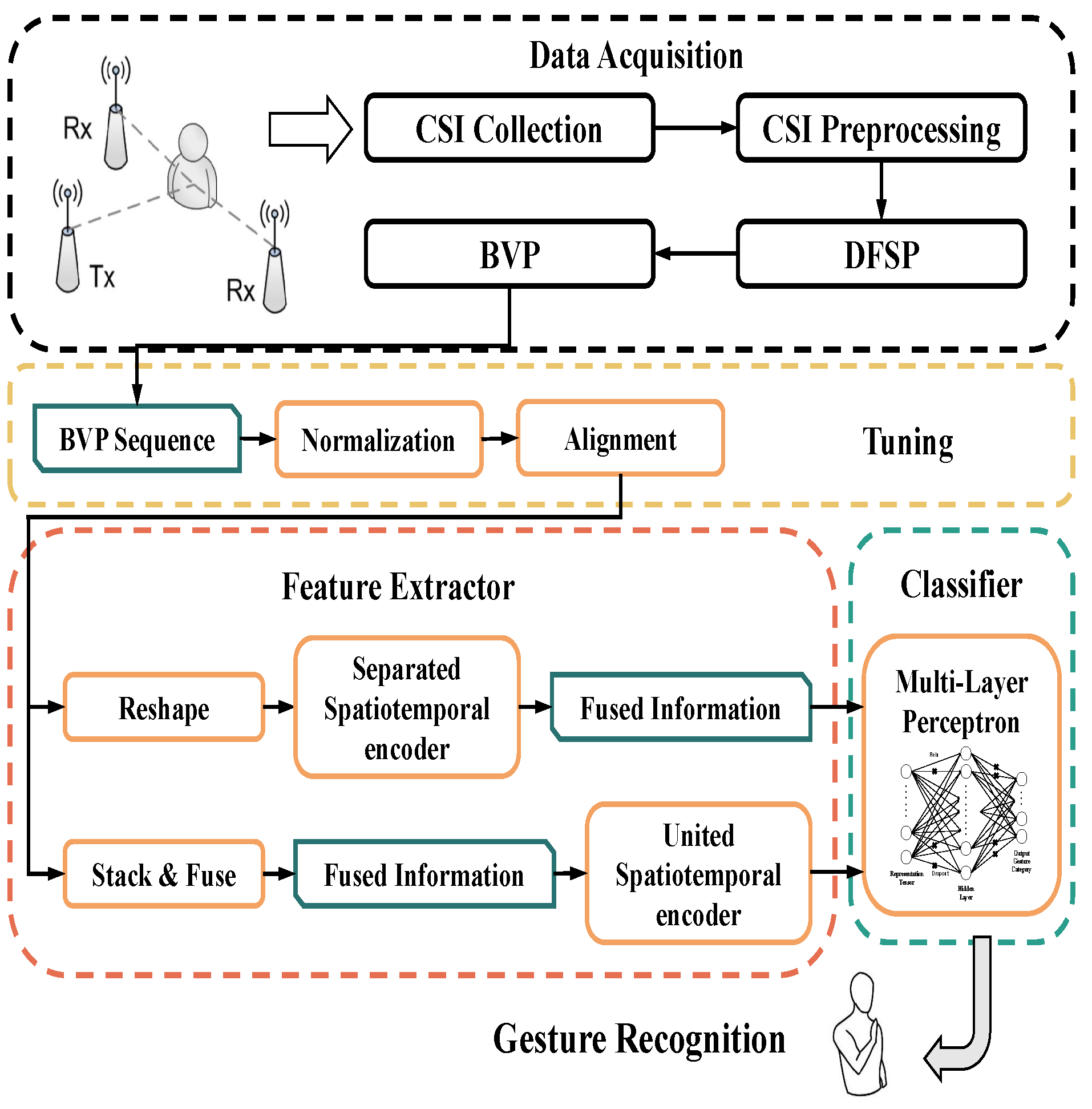
4.1. System Overview
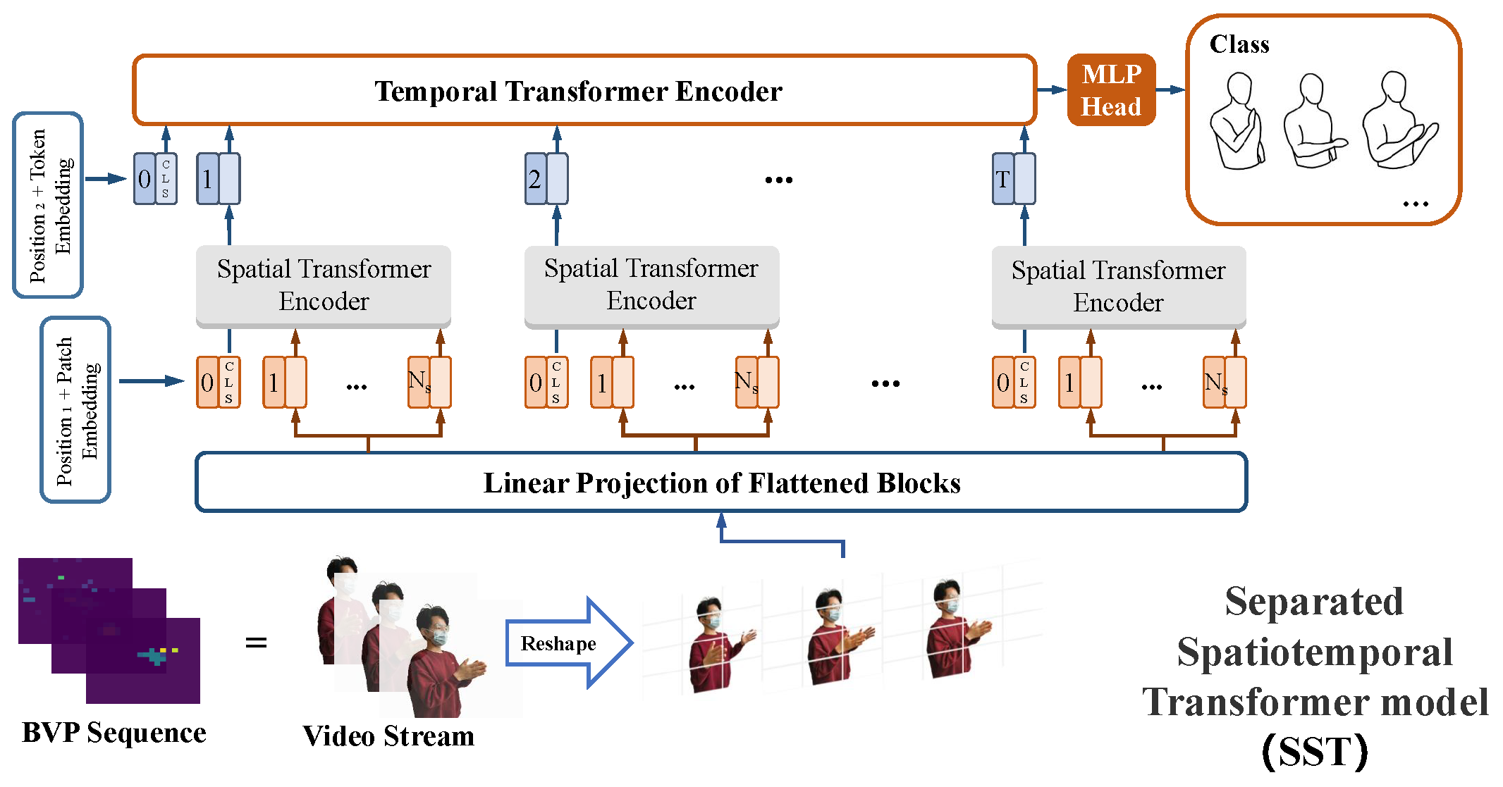
4.2. Separated Spatiotemporal Model
4.3. United Spatiotemporal Model
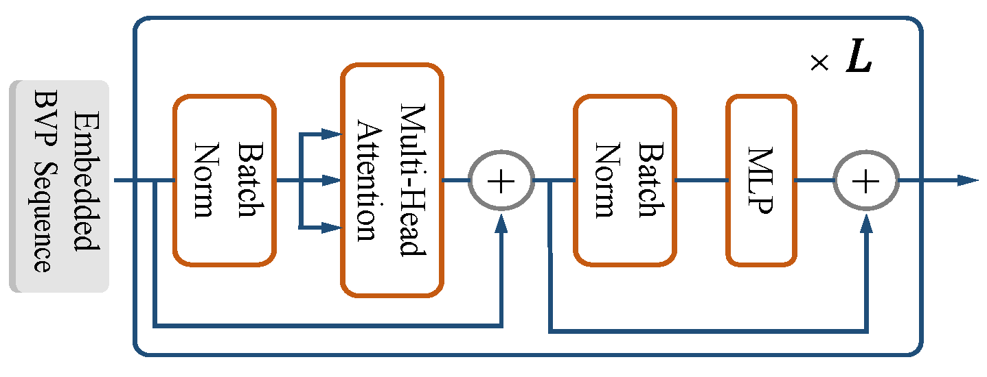
4.4. Encoder
4.5. Classifier
5. Evaluation and Discussion
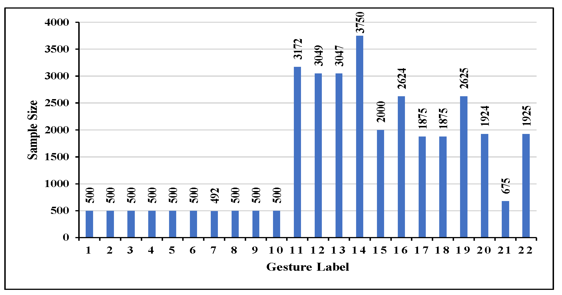
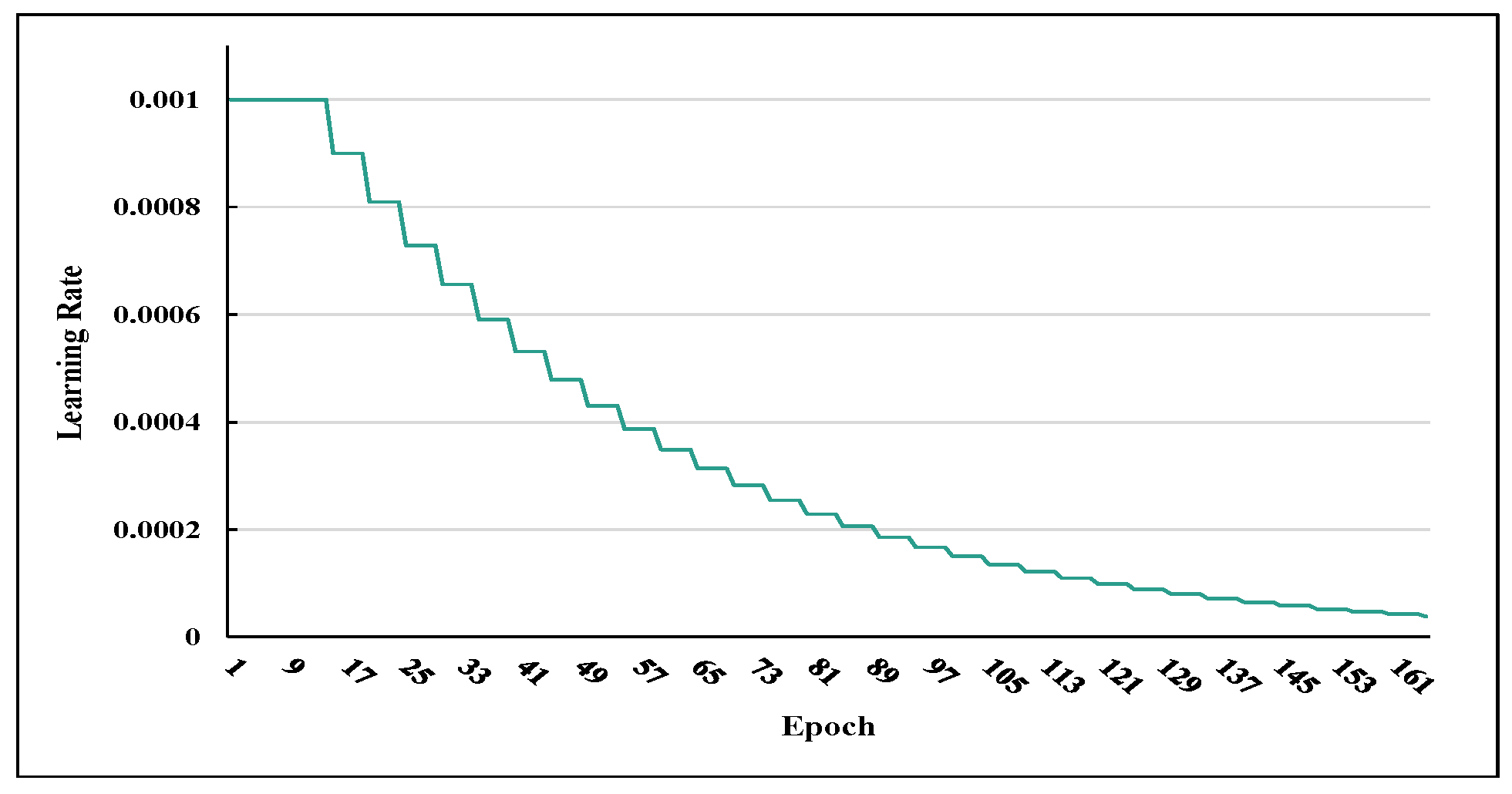
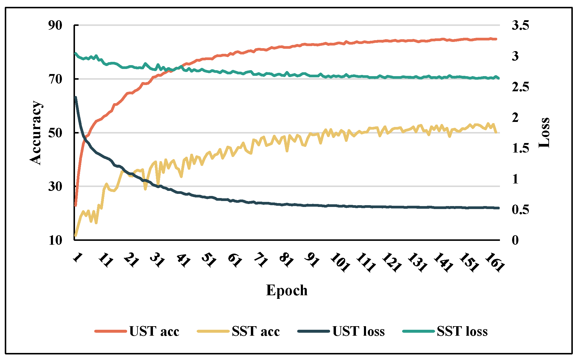
5.1. Experiments
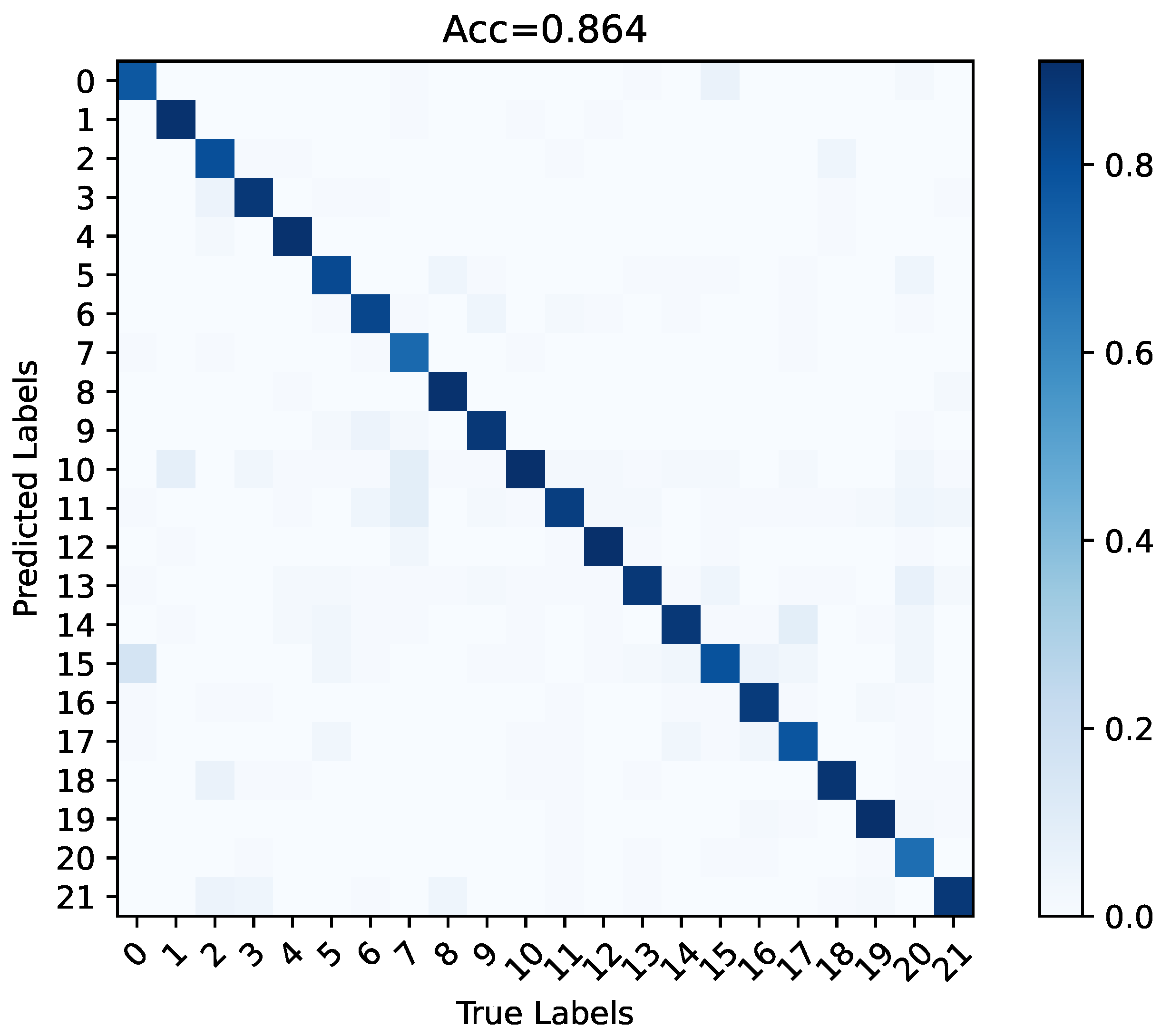
5.2. Effectiveness
5.3. Model Comparison
5.3.1. Accuracy and Robustness
5.3.2. Efficiency and Complexity
5.4. Comparison with State-of-the-Art
5.5. Ablation
5.5.1. Module Ablation
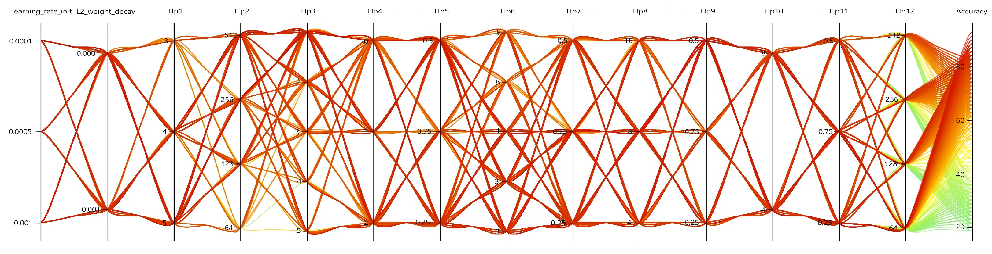
5.5.2. Hyperparameter Ablation
6. Conclusions
Author Contributions
Funding
Institutional Review Board Statement
Informed Consent Statement
Data Availability Statement
Acknowledgments
Conflicts of Interest
Abbreviations
| AL | Adversarial Learning |
| AOA | Angle of Arrival |
| BCS | Body Local Coordinate System |
| BN | Batch Normalization |
| BVP | Body-coordinate Velocity Profile |
| CFR | Channel Frequency Response |
| CNN | Convolutional Neural Networks |
| COTS | Commercial Off-the-Shelf |
| CPE | Channel Position Embedding |
| CRNN | The Model Combined CNN with RNN |
| CSI | Channel State Information |
| CV | Computer Vision |
| DL | Deep Learning |
| DFS | Doppler Frequency Shift |
| DFSP | Doppler Frequency Shift Profile |
| ECS | Environmental Global Coordinate System |
| GRU | The Gated Recurrent Units Neural Network |
| HAR | Human Activity Recognition |
| HGR | Human Gesture Recognition |
| HMM | Hidden Markov Mode |
| LoS | Line-of-Sight |
| LRCN | Long-term Recurrent Convolutional Networks |
| ML | Machine Learning |
| MLP | Multi-Layer Perception |
| MSA | Multi-head Self-Attention |
| NIC | Network Interface Card |
| NLoS | Non-Line-of-Sight |
| NLP | Natural Language Processing |
| nD | n-Dimensional |
| OFDM | Orthogonal Frequency Division Multiplexing |
| PCA | Principal Component Analysis |
| PE | Position Encoding |
| RNN | Recurrent Neural Networks |
| RSSI | Received Signal Strength Indication |
| SA | Self-Attention |
| SD | Standard Deviation |
| SE | Spatiotemporal Encoder |
| SST | Separated Spatiotemporal Transformer Model |
| TDSs | Task Datasets |
| TL | Transfer Learning |
| TOF | Time of Flight |
| UST | United Spatiotemporal Transformer model |
| ViT | Vision Transformer |
Appendix A

References
- Wang, Y.; Wu, K.; Ni, L.M. Wifall: Device-free fall detection by wireless networks. IEEE Trans. Mob. Comput. 2016, 16, 581–594. [Google Scholar] [CrossRef]
- Wang, T.; Wang, Z.; Zhang, D.; Gu, T.; Ni, H.; Jia, J.; Zhou, X.; Lv, J. Recognizing parkinsonian gait pattern by exploiting fine-grained movement function features. ACM Trans. Intell. Syst. Technol. (TIST) 2016, 8, 6. [Google Scholar] [CrossRef]
- Rana, R.; Kusy, B.; Wall, J.; Hu, W. Novel activity classification and occupancy estimation methods for intelligent HVAC (heating, ventilation and air conditioning) systems. Energy 2015, 93, 245–255. [Google Scholar] [CrossRef]
- Lai, J. The Development Research of Gesture Recognition Based on Human Interaction. In Cyber Security Intelligence and Analytics 2020; Springer: Berlin/Heidelberg, Germany, 2019; pp. 1175–1181. [Google Scholar]
- Wang, T.; Huang, W. Research on the Developmental Trend of Wearable Devices from the Perspective of Human-Computer Interaction. In Proceedings of the 6th International Conference on Electronic, Mechanical, Information and Management Society, Shenyang, China, 1–3 April 2016; Atlantis Press: Paris, France, 2016; pp. 770–774. [Google Scholar]
- Wang, W.; Liu, A.X.; Shahzad, M.; Ling, K.; Lu, S. Understanding and modeling of wifi signal based human activity recognition. In Proceedings of the 21st Annual International Conference on Mobile Computing and Networking, Paris, France, 7–11 September 2015; pp. 65–76. [Google Scholar]
- Chen, Z.; Zou, H.; Jiang, H.; Zhu, Q.; Soh, Y.C.; Xie, L. Fusion of WiFi, smartphone sensors and landmarks using the Kalman filter for indoor localization. Sensors 2015, 15, 715–732. [Google Scholar] [CrossRef]
- Abdelnasser, H.; Youssef, M.; Harras, K.A. Wigest: A ubiquitous wifi-based gesture recognition system. In Proceedings of the 2015 IEEE Conference on Computer Communications (INFOCOM), Hong Kong, China, 26 April–1 May 2015; pp. 1472–1480. [Google Scholar]
- Qian, K.; Wu, C.; Zhang, Y.; Zhang, G.; Yang, Z.; Liu, Y. Widar2. 0: Passive human tracking with a single Wi-Fi link. In Proceedings of the 16th Annual International Conference on Mobile Systems, Applications, and Services, Munich, Germany, 10–15 June 2018; pp. 350–361. [Google Scholar]
- Li, X.; Zhang, D.; Lv, Q.; Xiong, J.; Li, S.; Zhang, Y.; Mei, H. IndoTrack: Device-free indoor human tracking with commodity Wi-Fi. Proc. ACM Interact. Mob. Wearable Ubiquitous Technol. 2017, 1, 1–22. [Google Scholar] [CrossRef]
- Qian, K.; Wu, C.; Yang, Z.; Liu, Y.; Jamieson, K. Widar: Decimeter-level passive tracking via velocity monitoring with commodity Wi-Fi. In Proceedings of the 18th ACM International Symposium on Mobile Ad Hoc Networking and Computing, Chennai, India, 10–14 July 2017; pp. 1–10. [Google Scholar]
- Li, C.L.; Liu, M.; Cao, Z. WiHF: Gesture and user recognition with WiFi. IEEE Trans. Mob. Comput. 2020, 21, 757–768. [Google Scholar] [CrossRef]
- Zhang, Y.; Zheng, Y.; Qian, K.; Zhang, G.; Liu, Y.; Wu, C.; Yang, Z. Widar3. 0: Zero-effort cross-domain gesture recognition with wi-fi. IEEE Trans. Pattern Anal. Mach. Intell. 2021, 44, 8671–8688. [Google Scholar]
- Zeng, Y.; Wu, D.; Gao, R.; Gu, T.; Zhang, D. FullBreathe: Full human respiration detection exploiting complementarity of CSI phase and amplitude of WiFi signals. Proc. ACM Interact. Mob. Wearable Ubiquitous Technol. 2018, 2, 1–19. [Google Scholar] [CrossRef]
- Chen, Z.; Zhang, L.; Jiang, C.; Cao, Z.; Cui, W. WiFi CSI based passive human activity recognition using attention based BLSTM. IEEE Trans. Mob. Comput. 2018, 18, 2714–2724. [Google Scholar] [CrossRef]
- Yang, J.; Zou, H.; Zhou, Y.; Xie, L. Learning gestures from WiFi: A Siamese recurrent convolutional architecture. IEEE Internet Things J. 2019, 6, 10763–10772. [Google Scholar] [CrossRef]
- Guo, L.; Zhang, H.; Wang, C.; Guo, W.; Diao, G.; Lu, B.; Lin, C.; Wang, L. Towards CSI-based diversity activity recognition via LSTM-CNN encoder-decoder neural network. Neurocomputing 2021, 444, 260–273. [Google Scholar] [CrossRef]
- Shi, Z.; Cheng, Q.; Zhang, J.A.; Da Xu, R.Y. Environment-Robust WiFi-Based Human Activity Recognition Using Enhanced CSI and Deep Learning. IEEE Internet Things J. 2022, 9, 24643–24654. [Google Scholar] [CrossRef]
- Zhang, X.; Tang, C.; Yin, K.; Ni, Q. WiFi-Based Cross-Domain Gesture Recognition via Modified Prototypical Networks. IEEE Internet Things J. 2021, 9, 8584–8596. [Google Scholar] [CrossRef]
- Islam, M.S.; Jannat, M.K.A.; Hossain, M.N.; Kim, W.S.; Lee, S.W.; Yang, S.H. STC-NLSTMNet: An Improved Human Activity Recognition Method Using Convolutional Neural Network with NLSTM from WiFi CSI. Sensors 2023, 23, 356. [Google Scholar] [CrossRef]
- Vaswani, A.; Shazeer, N.; Parmar, N.; Uszkoreit, J.; Jones, L.; Gomez, A.N.; Kaiser, Ł.; Polosukhin, I. Attention is all you need. In Proceedings of the 30th International Conference on Neural Information Processing Systems, Long Beach, CA, USA, 4–9 December 2017. [Google Scholar]
- Li, B.; Cui, W.; Wang, W.; Zhang, L.; Chen, Z.; Wu, M. Two-stream convolution augmented transformer for human activity recognition. In Proceedings of the AAAI Conference on Artificial Intelligence, Virtually, 2–9 February 2021; Volume 35, pp. 286–293. [Google Scholar]
- Li, S.; Ge, Y.; Shentu, M.; Zhu, S.; Imran, M.; Abbasi, Q.; Cooper, J. Human Activity Recognition based on Collaboration of Vision and WiFi Signals. In Proceedings of the 2021 International Conference on UK-China Emerging Technologies (UCET), Chengdu, China, 4–6 November 2021; pp. 204–208. [Google Scholar]
- Gu, Z.; He, T.; Wang, Z.; Xu, Y. Device-Free Human Activity Recognition Based on Dual-Channel Transformer Using WiFi Signals. Wirel. Commun. Mob. Comput. 2022, 2022, 4598460. [Google Scholar] [CrossRef]
- Abdel-Basset, M.; Hawash, H.; Moustafa, N.; Mohammad, N. H2HI-Net: A Dual-Branch Network for Recognizing Human-to-Human Interactions from Channel-State-Information. IEEE Internet Things J. 2021, 9, 10010–10021. [Google Scholar] [CrossRef]
- Gu, Y.; Zhang, X.; Wang, Y.; Wang, M.; Yan, H.; Ji, Y.; Liu, Z.; Li, J.; Dong, M. WiGRUNT: WiFi-enabled gesture recognition using dual-attention network. IEEE Trans. Hum.-Mach. Syst. 2022, 52, 736–746. [Google Scholar] [CrossRef]
- Wiseman, Y.; Fredj, E. Contour extraction of compressed JPEG images. J. Graph. Tools 2001, 6, 37–43. [Google Scholar] [CrossRef]
- Dubuisson, M.P.; Jain, A.K. Contour extraction of moving objects in complex outdoor scenes. Int. J. Comput. Vis. 1995, 14, 83–105. [Google Scholar] [CrossRef]
- Kim, N.; Kim, D.; Lan, C.; Zeng, W.; Kwak, S. Restr: Convolution-free referring image segmentation using transformers. In Proceedings of the IEEE/CVF Conference on Computer Vision and Pattern Recognition, New Orleans, LA, USA, 18–24 June 2022; pp. 18145–18154. [Google Scholar]
- Zaidi, S.S.A.; Ansari, M.S.; Aslam, A.; Kanwal, N.; Asghar, M.; Lee, B. A survey of modern deep learning based object detection models. Digit. Signal Process. 2022, 126, 103514. [Google Scholar] [CrossRef]
- Niu, K.; Zhang, F.; Chang, Z.; Zhang, D. A fresnel diffraction model based human respiration detection system using COTS Wi-Fi devices. In Proceedings of the 2018 ACM International Joint Conference and 2018 International Symposium on Pervasive and Ubiquitous Computing and Wearable Computers, Singapore, 8–12 October 2018; pp. 416–419. [Google Scholar]
- Li, X.; Li, S.; Zhang, D.; Xiong, J.; Wang, Y.; Mei, H. Dynamic-music: Accurate device-free indoor localization. In Proceedings of the 2016 ACM International Joint Conference on Pervasive and Ubiquitous Computing, Heidelberg, Germany, 12–16 September 2016; pp. 196–207. [Google Scholar]
- Joshi, K.; Bharadia, D.; Kotaru, M.; Katti, S. WiDeo: Fine-grained Device-free Motion Tracing using RF Backscatter. In Proceedings of the 12th USENIX Symposium on Networked Systems Design and Implementation (NSDI 15), Boston, MA, USA, 26–28 February 2015; pp. 189–204. [Google Scholar]
- Zhang, F.; Niu, K.; Xiong, J.; Jin, B.; Gu, T.; Jiang, Y.; Zhang, D. Towards a diffraction-based sensing approach on human activity recognition. Proc. ACM Interact. Mob. Wearable Ubiquitous Technol. 2019, 3, 1–25. [Google Scholar] [CrossRef]
- Wang, W.; Liu, A.X.; Shahzad, M.; Ling, K.; Lu, S. Device-free human activity recognition using commercial WiFi devices. IEEE J. Sel. Areas Commun. 2017, 35, 1118–1131. [Google Scholar] [CrossRef]
- Wang, Y.; Liu, J.; Chen, Y.; Gruteser, M.; Yang, J.; Liu, H. E-eyes: Device-free location-oriented activity identification using fine-grained wifi signatures. In Proceedings of the 20th Annual International Conference on Mobile Computing and Networking, Maui, HI, USA, 7–11 September 2014; pp. 617–628. [Google Scholar]
- Ali, K.; Liu, A.X.; Wang, W.; Shahzad, M. Keystroke recognition using wifi signals. In Proceedings of the 21st Annual International Conference on Mobile Computing and Networking, Paris, France, 7–11 September 2015; pp. 90–102. [Google Scholar]
- Wang, H.; Zhang, D.; Wang, Y.; Ma, J.; Wang, Y.; Li, S. RT-Fall: A real-time and contactless fall detection system with commodity WiFi devices. IEEE Trans. Mob. Comput. 2016, 16, 511–526. [Google Scholar] [CrossRef]
- Sun, Z.; Ke, Q.; Rahmani, H.; Bennamoun, M.; Wang, G.; Liu, J. Human action recognition from various data modalities: A review. IEEE Trans. Pattern Anal. Mach. Intell. 2022, 45, 3200–3225. [Google Scholar] [CrossRef]
- Jiang, W.; Miao, C.; Ma, F.; Yao, S.; Wang, Y.; Yuan, Y.; Xue, H.; Song, C.; Ma, X.; Koutsonikolas, D.; et al. Towards environment independent device free human activity recognition. In Proceedings of the 24th Annual International Conference on Mobile Computing and Networking, New Delhi, India, 29 October–2 November 2018; pp. 289–304. [Google Scholar]
- Zhang, J.; Tang, Z.; Li, M.; Fang, D.; Nurmi, P.; Wang, Z. CrossSense: Towards cross-site and large-scale WiFi sensing. In Proceedings of the 24th Annual International Conference on Mobile Computing and Networking, New Delhi, India, 29 October–2 November 2018; pp. 305–320. [Google Scholar]
- Yang, J.; Chen, X.; Wang, D.; Zou, H.; Lu, C.X.; Sun, S.; Xie, L. Deep learning and its applications to WiFi human sensing: A benchmark and a tutorial. arXiv 2022, arXiv:2207.07859. [Google Scholar]
- Jolliffe, I.T.; Cadima, J. Principal component analysis: A review and recent developments. Philos. Trans. R. Soc. A: Math. Phys. Eng. Sci. 2016, 374, 20150202. [Google Scholar] [CrossRef]
- Yan, S.; Shao, H.; Xiao, Y.; Liu, B.; Wan, J. Hybrid robust convolutional autoencoder for unsupervised anomaly detection of machine tools under noises. Robot. Comput.-Integr. Manuf. 2023, 79, 102441. [Google Scholar] [CrossRef]
- Mikolov, T.; Chen, K.; Corrado, G.; Dean, J. Efficient estimation of word representations in vector space. arXiv 2013, arXiv:1301.3781. [Google Scholar]
- Yağ, İ.; Altan, A. Artificial Intelligence-Based Robust Hybrid Algorithm Design and Implementation for Real-Time Detection of Plant Diseases in Agricultural Environments. Biology 2022, 11, 1732. [Google Scholar] [CrossRef]
- Sezer, A.; Altan, A. Detection of solder paste defects with an optimization-based deep learning model using image processing techniques. Solder. Surf. Mt. Technol. 2021, 33, 291–298. [Google Scholar] [CrossRef]
- Sezer, A.; Altan, A. Optimization of deep learning model parameters in classification of solder paste defects. In Proceedings of the 2021 3rd International Congress on Human-Computer Interaction, Optimization and Robotic Applications (HORA), Ankara, Turkey, 11–13 June 2021; pp. 1–6. [Google Scholar]
- Dosovitskiy, A.; Beyer, L.; Kolesnikov, A.; Weissenborn, D.; Zhai, X.; Unterthiner, T.; Dehghani, M.; Minderer, M.; Heigold, G.; Gelly, S.; et al. An image is worth 16×16 words: Transformers for image recognition at scale. arXiv 2020, arXiv:2010.11929. [Google Scholar]
- Arnab, A.; Dehghani, M.; Heigold, G.; Sun, C.; Lučić, M.; Schmid, C. Vivit: A video vision transformer. In Proceedings of the IEEE/CVF International Conference on Computer Vision, Montreal, BC, Canada, 11–17 October 2021; pp. 6836–6846. [Google Scholar]
- Guo, M.H.; Xu, T.X.; Liu, J.J.; Liu, Z.N.; Jiang, P.T.; Mu, T.J.; Zhang, S.H.; Martin, R.R.; Cheng, M.M.; Hu, S.M. Attention mechanisms in computer vision: A survey. Comput. Vis. Media 2022, 8, 331–368. [Google Scholar] [CrossRef]
- Donoho, D.L. Compressed sensing. IEEE Trans. Inf. Theory 2006, 52, 1289–1306. [Google Scholar] [CrossRef]
- Donahue, J.; Anne Hendricks, L.; Guadarrama, S.; Rohrbach, M.; Venugopalan, S.; Saenko, K.; Darrell, T. Long-term recurrent convolutional networks for visual recognition and description. In Proceedings of the IEEE Conference on Computer Vision and Pattern Recognition, Boston, MA, USA, 7–12 June 2015; pp. 2625–2634. [Google Scholar]
- Devlin, J.; Chang, M.W.; Lee, K.; Toutanova, K. Bert: Pre-training of deep bidirectional transformers for language understanding. arXiv 2018, arXiv:1810.04805. [Google Scholar]
- Gehring, J.; Auli, M.; Grangier, D.; Yarats, D.; Dauphin, Y.N. Convolutional sequence to sequence learning. In Proceedings of the International Conference on Machine Learning, PMLR, Sydney, Australia, 6–11 August 2017; pp. 1243–1252. [Google Scholar]
- Tran, D.; Bourdev, L.; Fergus, R.; Torresani, L.; Paluri, M. Learning spatiotemporal features with 3d convolutional networks. In Proceedings of the IEEE International Conference on Computer Vision, Santiago, Chile, 7–13 December 2015; pp. 4489–4497. [Google Scholar]
- Ioffe, S.; Szegedy, C. Batch normalization: Accelerating deep network training by reducing internal covariate shift. In Proceedings of the International Conference on Machine Learning, PMLR, Lille, France, 7–9 July 2015; pp. 448–456. [Google Scholar]
- Baevski, A.; Auli, M. Adaptive input representations for neural language modeling. arXiv 2018, arXiv:1809.10853. [Google Scholar]
- Paszke, A.; Gross, S.; Massa, F.; Lerer, A.; Bradbury, J.; Chanan, G.; Killeen, T.; Lin, Z.; Gimelshein, N.; Antiga, L.; et al. PyTorch: An Imperative Style, High-Performance Deep Learning Library. In Advances in Neural Information Processing Systems 32; Curran Associates, Inc.: New York, NY, USA, 2019; pp. 8024–8035. [Google Scholar]
- Yang, Z.; Zhang, Y.; Zhang, G.; Zheng, Y. Widar 3.0: WiFi-based activity recognition dataset. IEEE Dataport 2020. [Google Scholar] [CrossRef]
- Lin, T.Y.; Maire, M.; Belongie, S.; Hays, J.; Perona, P.; Ramanan, D.; Dollár, P.; Zitnick, C.L. Microsoft coco: Common objects in context. In Proceedings of the European Conference on Computer Vision, Zurich, Switzerland, 6–12 September 2014; Springer: Berlin/Heidelberg, Germany, 2014; pp. 740–755. [Google Scholar]
- Deng, J.; Dong, W.; Socher, R.; Li, L.J.; Li, K.; Fei-Fei, L. Imagenet: A large-scale hierarchical image database. In Proceedings of the 2009 IEEE Conference on Computer Vision and Pattern Recognition, Miami, FL, USA, 20–25 June 2009; pp. 248–255. [Google Scholar]
- He, K.; Zhang, X.; Ren, S.; Sun, J. Delving deep into rectifiers: Surpassing human-level performance on imagenet classification. In Proceedings of the IEEE International Conference on Computer Vision, Santiago, Chile, 7–13 December 2015; pp. 1026–1034. [Google Scholar]
- Sun, C.; Shrivastava, A.; Singh, S.; Gupta, A. Revisiting unreasonable effectiveness of data in deep learning era. In Proceedings of the IEEE International Conference on Computer Vision, Venice, Italy, 22–29 October 2017; pp. 843–852. [Google Scholar]
- Diba, A.; Fayyaz, M.; Sharma, V.; Karami, A.H.; Arzani, M.M.; Yousefzadeh, R.; Van Gool, L. Temporal 3d convnets: New architecture and transfer learning for video classification. arXiv 2017, arXiv:1711.08200. [Google Scholar]
- Ji, S.; Xu, W.; Yang, M.; Yu, K. 3D convolutional neural networks for human action recognition. IEEE Trans. Pattern Anal. Mach. Intell. 2012, 35, 221–231. [Google Scholar] [CrossRef]
- Hutter, F.; Hoos, H.H.; Leyton-Brown, K. Sequential model-based optimization for general algorithm configuration. In Proceedings of the International Conference on Learning and Intelligent Optimization, Rome, Italy, 17–21 January 2011; Springer: Berlin/Heidelberg, Germany, 2011; pp. 507–523. [Google Scholar]
- Microsoft. Neural Network Intelligence. 2021. Available online: https://github.com/microsoft/nni (accessed on 14 January 2021).


| Method | Task | Model | DataType |
|---|---|---|---|
| EI [40] | HGR | Adversarial Generative networks | CSI |
| CrossSense [41] | HGR | Roaming model (Transfer Learning) | CSI |
| Ref. [15] | HAR | BLSTM | CSI |
| WIHF [12] | Human Identification Gesture Recognition | CNN+GRU | DFS |
| Widar 3.0 [13] | HGR | CNN+GRU | BVP |
| LCED [17] | HAR | CNN+GRU | CSI |
| THAT [22] | HAR | Transformers (Two-stream) | CSI |
| WiGr [19] | HGR | Prototypical Networks | CSI |
| Ref. [24] | HGR | Transformers | CSI |
| WiGRUNT [26] | HGR | CNN (Attention) | CSI |
| SenseFi [42] | HAR, HGR | ResNet, LSTM Transformers | CSI, BVP |
| STC-NLSTMNet [20] | HAR | CNN+NLSTM | CSI |
| AFEE [18] | HAR | MatNet | CSI |
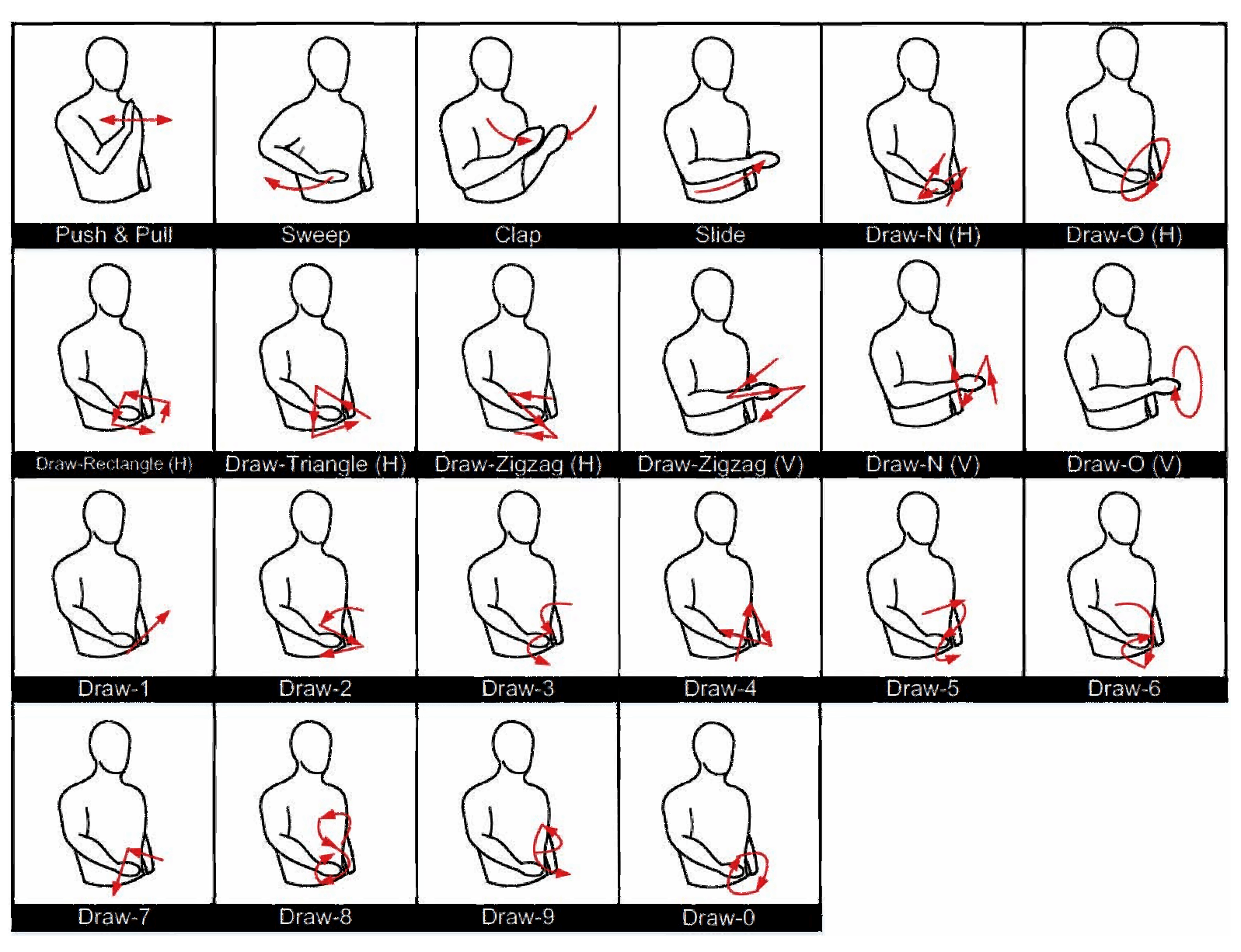
| Gesture | Label | Gesture | Label | Gesture | Label |
|---|---|---|---|---|---|
| Draw-0 | 0 | Draw-8 | 8 | Draw-Rectangle (H) | 16 |
| Draw-1 | 1 | Draw-9 | 9 | Draw-Triangle (H) | 17 |
| Draw-2 | 2 | Push and Pull | 10 | Draw-Z (H) | 18 |
| Draw-3 | 3 | Sweep | 11 | Draw-N (V) | 19 |
| Draw-4 | 4 | Clap | 12 | Draw-O (V) | 20 |
| Draw-5 | 5 | Slide | 13 | Draw-Z (V) | 21 |
| Draw-6 | 6 | Draw-N (H) | 14 | ||
| Draw-7 | 7 | Draw-O (H) | 15 |
| TDSs | Classification | Similarity | Distortion | Data Imbalance |
|---|---|---|---|---|
| TDSs-6 | 6 | 0 | 0 | 380.09 |
| TDSs-9 | 9 | 4 | 0 | 1223.80 |
| TDSs-12 | 12 | 2 | 3 | 790.18 |
| TDSs-22 | 22 | 4 | 3 | 1102.79 |
| Task Dataset | Gesture |
|---|---|
| TDSs-6 | Push and Pull, Sweep, Clap, Slide, Draw-O (H), Draw-Z (H) |
| TDSs-9 | Draw-0, Draw-O; Draw-1, Slide, Sweep; Draw-2, Draw-Z (H); Draw-4, Draw-Triangle (H) |
| TDSs-12 | Push and Pull, Sweep, Clap, Slide, Draw-O (H), Draw-Z (H), Draw-N (H), Draw-Rectangle (H), Draw-Triangle (H), Draw-N(V), Draw-O (V), Draw-Z (V) |
| TDSs-22 | Draw-0, Draw-1, Draw-2, Draw-3, Draw-4, Draw-5, Draw-6, Draw-7, Draw-8, Draw-9, Push and Pull, Sweep, Clap, Slide, Draw-O (H), Draw-Z (H), Draw-N (H), Draw-O (V),Draw-Z (V), Draw-N (V) |
| Module | Hyperparameter | Value | Label |
|---|---|---|---|
| Stacking-Fusion | Tube size | h = 2, w = 2, t = | Hp1 |
| Tube Embedding Dimension (D) | 256 | Hp2 | |
| Tube Stride | 2 | Hp3 | |
| Tube Padding | 0 | Hp4 | |
| Dropout Ratio 1 | 0.75 | Hp5 | |
| Spatiotemporal Encoder | Spatiotemporal Layer Number | 1 | Hp6 |
| Droupout Ratio 2 | 0.25 | Hp7 | |
| MSA Head Number | 16 | Hp8 | |
| MSA Dropout Ratio | 0.25 | Hp9 | |
| MLP Hidden Dimension | 4 × 256 | Hp10 | |
| MLP Output Dimension | 256 | Hp2 | |
| Dropout Ratio 3 | 0.25 | Hp11 | |
| MLP Classifier | MLP Projection Dimension () | 16 | Hp12 |
| Model Type | TDSs-6 | TDSs-9 | TDSs-12 | TDSs-22 |
|---|---|---|---|---|
| UST | 0.8731 | 0.8538 | 0.8501 | 0.8531 |
| SST | 0.7314 | 0.0 | 0.4122 | 0.5128 |
| CNN+GRU | 0.8633 | 0.7940 | 0.6034 | 07319 |
| CNN+LSTM | 0.8726 | 0.7950 | 0.6094 | 0.7147 |
| Conv2D | 0.8701 | 0.8496 | 0.8165 | 0.8227 |
| Conv3D | 0.8947 | 0.8640 | 0.8353 | 0.8411 |
| Model Type | |
|---|---|
| UST | −3.18% |
| SST | −21.42% |
| CNN+GRU | −21.24% |
| CNN+LSTM | −15.08% |
| Conv2D | −7.29% |
| Conv3D | −7.08% |
| Model | FLOPs | Parameters | Time (CPU) | Memory (CPU) |
|---|---|---|---|---|
| UST | 56.37 M | 0.69 M | 11.77 ms | 3.80 Mb |
| SST | 105.65 M | 3.29 M | 55.93 ms | 16.61 Mb |
| CNN+GRU | 34.96 M | 0.84 M | 991.88 ms | 3.25 Mb |
| CNN+LSTM | 37.73 M | 0.94 M | 981.25 ms | 3.63 Mb |
| Conv2D | 12 M | 0.58 M | 7.10 ms | 6.21 Mb |
| Conv3D | 25.13 M | 12.85 M | 21.70 ms | 49.06 Mb |
| Computing Module | Model Complexity | Sequential Operations | Backbone |
|---|---|---|---|
| Self-Attention | UST | ||
| Self-Attention × 2 | SST | ||
| Recurrent | - | ||
| 2D Convolutional | Conv2D | ||
| 3D Convolutional | Conv3D | ||
| CRNN | CNN+LSTM, CNN+GRU |
| Module | Accuracy | Delta () |
|---|---|---|
| UST | 89.34% | - |
| - Dropout | 66.58% | −22.76% |
| - BN | 16.34% | −73% |
| - Learnable PE | 68.61% | −20.73% |
| - CPE | 85.58% | −3.76% |
| Model | CPE | No CPE |
|---|---|---|
| UST | 89.34% | 85.58% |
| Conv2D | 87.81% | 84.96% |
| Hyperparameters | CNN+LSTM | CNN+GRU | Conv3D | Conv2D |
|---|---|---|---|---|
| LR_init | [0.0001, 0.00002, 0.00001] | [0.0001, 0.00002, 0.00001] | [0.005, 0.001, 0.0002] | [0.0002, 0.00005, 0.00001] |
| weight decay | [0.001, 0.0001, 0.00005] | [0.001, 0.0001, 0.00005] | [0.001, 0.0001, 0.00005] | [0.001, 0.0001, 0.00005] |
| Gamma | [0.9 0.7 0.5] | [0.9 0.7 0.5] | [0.9 0.7 0.5] | [0.9 0.7 0.5] |
| kernel size | [5, 3, 1] | [5, 3, 1] | [5, 3, 1] | [5, 3, 1] |
| stride | [1, 2, 4] | [1, 2, 4] | [1, 2, 4] | [1, 2, 4] |
| dimension-1 | [16, 64, 256] | [16, 64, 256] | [16, 64, 256] | [16, 64, 256] |
| maxpooling | [2, 4] | [2, 4] | [2, 4] | [2, 4] |
| FC dimension-1 | [128, 256, 512, 1024] | [128, 256, 512, 1024] | [128, 256, 512, 1024] | [128, 256, 512, 1024] |
| drop ratio-1 | [0.25, 0.5, 0.75] | [0.25, 0.5, 0.75] | [0.25, 0.5, 0.75] | [0.25, 0.5, 0.75] |
| FC dimension-2 | [64, 128, 256] | [64, 128, 256] | [64, 128, 256] | [64, 128, 256] |
| Blk_num-1 | [1, 4, 8] | [1, 4, 8] | [1, 4, 8] | [1, 4, 8] |
| dimension-2 | [64, 128, 256] | [64, 128, 256] | - | - |
| drop ratio-2 | [0.25, 0.5, 0.75] | [0.25, 0.5, 0.75] | - | - |
| Blk_num-2 | [1, 4, 8] | [1, 4, 8] | - | - |
| Act.Fun. | ReLu | |||
Disclaimer/Publisher’s Note: The statements, opinions and data contained in all publications are solely those of the individual author(s) and contributor(s) and not of MDPI and/or the editor(s). MDPI and/or the editor(s) disclaim responsibility for any injury to people or property resulting from any ideas, methods, instructions or products referred to in the content. |
© 2023 by the authors. Licensee MDPI, Basel, Switzerland. This article is an open access article distributed under the terms and conditions of the Creative Commons Attribution (CC BY) license (https://creativecommons.org/licenses/by/4.0/).
Share and Cite
Yang, M.; Zhu, H.; Zhu, R.; Wu, F.; Yin, L.; Yang, Y. WiTransformer: A Novel Robust Gesture Recognition Sensing Model with WiFi. Sensors 2023, 23, 2612. https://doi.org/10.3390/s23052612
Yang M, Zhu H, Zhu R, Wu F, Yin L, Yang Y. WiTransformer: A Novel Robust Gesture Recognition Sensing Model with WiFi. Sensors. 2023; 23(5):2612. https://doi.org/10.3390/s23052612
Chicago/Turabian StyleYang, Mingze, Hai Zhu, Runzhe Zhu, Fei Wu, Ling Yin, and Yuncheng Yang. 2023. "WiTransformer: A Novel Robust Gesture Recognition Sensing Model with WiFi" Sensors 23, no. 5: 2612. https://doi.org/10.3390/s23052612
APA StyleYang, M., Zhu, H., Zhu, R., Wu, F., Yin, L., & Yang, Y. (2023). WiTransformer: A Novel Robust Gesture Recognition Sensing Model with WiFi. Sensors, 23(5), 2612. https://doi.org/10.3390/s23052612